Transverse instabilities of stripe domains in magnetic thin films with perpendicular magnetic anisotropy
Abstract
Stripe domains are narrow, elongated, reversed regions that exist in magnetic materials with perpendicular magnetic anisotropy. Stripe domains appear as a pair of domain walls that can exhibit topology with a nonzero chirality. Recent experimental and numerical investigations identify an instability of stripe domains in the long direction as a means of nucleating isolated magnetic skyrmions. Here, the onset and nonlinear evolution of transverse instabilities for a dynamic stripe domain known as the bion stripe are investigated. Both non-topological and topological variants of the bion stripe are shown to exhibit a long-wavelength transverse instability with different characteristic features. In the former, small transverse variations in the stripe’s width lead to a neck instability that eventually pinches the non-topological stripe into a chain of two-dimensional breathers composed of droplet soliton pairs. In the latter case, small variations in the stripe’s center results in a snake instability whose topological structure leads to the nucleation of dynamic magnetic skyrmions and antiskyrmions as well as perimeter-modulated droplets. Quantitative, analytical predictions for both the early, linear evolution and the long-time, nonlinear evolution are achieved using an averaged Lagrangian approach that incorporates both exchange (dispersion) and anisotropy (nonlinearity). The method of analysis is general and can be applied to other filamentary structures.
I Introduction
Solitons [1] are localized structures that are ubiquitous in nonlinear media such as fiber optics [2], water waves [3] or atomic condensates [4]. In general, solitons manifest a balance between nonlinearity and dispersion. Magnetic materials exhibit both nonlinearity and dispersion associated, respectively, with anisotropy and exchange. In their simplest manifestation, solitons in magnetic materials correspond to one-dimensional domain walls that separate well-defined magnetic states or domains [5]. Domain wall nucleation and motion can be manipulated in nanowires, a feature that has led to the proposal of domain-wall-based technology for oscillators [6], magnonics [7, 8], and computation [9, 10]. It is also possible for a pair of domain walls to form a dynamically precessing bound state known as a magnetic bion [11, 12].
Two-dimensional solitons can also exist in magnetic materials with uniaxial anisotropy balancing exchange. Uniaxial anisotropy is typically achieved in hard magnetic alloys [13] or ultra-thin film multilayers [14, 15], and is commonly referred to as perpendicular magnetic anisotropy (PMA). In these materials, it has been possible to observe two-dimensional solitons such as dissipative droplets [16, 17, 18, 19, 20] and skyrmions [21, 22, 23, 24, 25], finding potential applications as oscillators [26] and information carriers [27, 28], respectively.
An important figure-of-merit for magnetic solitons is their stability to perturbations. Topological concepts [12] can be utilized to predict certain aspects of the stability and dynamics of magnetic solitons. One-dimensional domain walls can be classified by their chirality , defined as[12]
| (1) |
where is the azimuthal angle of the magnetization’s in-plane component. The chirality describes the magnetization vector sense of rotation between two domains. Note that this definition of chirality is typically utilized to classify domain walls in planar ferromagnets whereas here, we are considering uniaxial ferromagnets. The reason we introduce the definition of chirality in (1) that counts the rotations of the in-plane magnetization component rather than one that counts rotations of the out-of-plane magnetization component is because the magnetic bion considered in this work always exhibits a positive and a canceling negative rotation in . The bion’s in-plane chirality (1) can be nonzero.
Two-dimensional solitons can be categorized into topological classes according to their skyrmion number[12]
| (2) |
that determines how many times the magnetization texture, defined by the magnetization vector , can be mapped onto a sphere. When the chirality and skyrmion number are zero, the state is considered non-topological or topologically trivial, and indicates that such a texture can be smoothly deformed or decays in the presence of magnetic damping to a spatially homogeneous state.
Magnetic soliton topology yields important information about the collective behavior of multiple solitons. For example, domain walls with opposite chirality can annihilate into a trivial, homogeneous state. Conversely, domain walls with equal chirality are topologically protected from annihilating. In magnetic materials with PMA, such domain wall bound states form into dynamically precessing non-topological and topological bions[11, 12] that, when extended transversely, are called bion stripes. In the absence of an applied field, the in-plane magnetization of a non-topological bion stripe exhibits a counter-clockwise precessional frequency that corresponds to a positive sign in conventional spin dynamics; topological bions exhibit clockwise or negative precessional frequency. In the case of localized, two-dimensional solitons, the additional degree of freedom also leads to richer behavior. Examples include the merging or annihilation of droplets [29], dynamical skyrmions in the presence of radially symmetric fields [26], and perimeter modulations of both textures [30, 31].
In realistic experiments and potential applications, topological protection can be compromised by the geometry of the system. Two-dimensional materials can be approximately achieved by utilizing films with a thickness smaller than the exchange length (on the order of nm), leading to a near-homogeneous magnetization along the thickness. However, one-dimensional magnetic materials require lateral confinement in the form of nanowires that are typically wider than the exchange length due to fabrication method limitations. Therefore, effectively one-dimensional magnetic solitons are prone to transverse dynamics as observed, e.g., in externally driven domain-wall motion [32, 33] and spin-transfer-torque-driven dissipative droplets [34] in nanowires. In a more extreme case, transverse dynamics can be unstable. Such an instability can be detrimental to domain-wall-based technologies, but can also be used to nucleate two-dimensional solitons, as shown both numerically and experimentally for single skyrmions in a series of recent works [23, 24, 35, 36, 37]. However, there is neither an analytical description of such an instability nor a systematic understanding of the number and topology of resultant two-dimensional textures. The transverse instability of quasi-one-dimensional structures is a subject of interest in its own right, as it can provide a control handle towards the design of configurations with a particular number of two-dimensional textures as has been proposed, e.g., for vortices in atomic Bose-Einstein condensates [38]. Nonlinear mathematical tools are needed that can account for both anisotropy and exchange. A particularly useful method is the average Lagrangian approach [39], where nonlinear dynamics of transverse soliton modulation can be analyzed. To investigate the stability of transverse dynamics, we utilize the average Lagrangian approach applied to bion stripes in a two-dimensional thin film with PMA.
In this paper, we show that bion stripes are transversely unstable in a manner that depends on their topology. The non-topological bion exhibits a symmetric or “neck” instability that eventually pinches and nucleates breathers composed of droplet pairs. The topological bion exhibits an antisymmetric or “snake” instability that nucleates a series of topological defects that evolve into droplets, skyrmions, and anti-skyrmions. The number of droplets and topological defects per unit length can be estimated by the most unstable transverse mode, which enables us to control the dynamical outcome of our numerical simulations. However, long time dynamics exhibit soliton interactions that fall outside the applicability of our analytical approach. The properties of the long-wavelength transverse instability allow us to determine a nanowire lateral confinement for which the bion stripe is stable. Our study introduces a method to analytically describe the nonlinear dynamics of stripe domains in magnetic materials.
The remainder of the paper is organized as follows. In Sec. II, we introduce the analytical model for magnetization dynamics and the analytical form of a bion stripe solution. The linear stability analysis of bion stripe transverse perturbations is studied in Sec. III using the average Lagrangian method and numerical linearization. In Sec. IV, the nonlinear evolution of a bion filament is studied and Sec. V presents numerical simulations detailing the filamentary breakup. A discussion of the implications of our analysis for stabilized bions in physically confined structures is presented in Sec. VI. Finally, we provide concluding remarks in Sec. VII.
II Analytical model
Magnetization dynamics can be analytically described over sufficiently short time scales by the conservative Larmor torque equation [11]
| (3) |
expressed here in dimensionless form by rescaling time, space, and fields such that . Time is scaled by where is the gyromagnetic ratio, is the vacuum permeability, and where is the uniaxial anisotropy constant and the saturation magnetization; space is scaled by where is the exchange length; and fields are scaled by . The effective field includes relevant physics for the magnetic system studied. Here, we consider a perpendicular external field , exchange field, and perpendicular uniaxial anisotropy
| (4) |
We assume a sufficiently thin and transversely extended film so that long-range dipolar fields are negligible and the magnetization does not vary through the film thickness, i.e., it is a two-dimensional magnet. The effective field can be described as the functional derivative of the magnetic energy density, (defined below), with respect to the magnetization vector.
For the following analysis, it is convenient to represent Eqs. (3) and (4) in spherical coordinates. For this, we introduce the transformation
| (5) |
where is the phase relative to the precession induced by the applied field and is the polar angle of the magnetization. In this coordinate system, the energy density can be written as [16]
| (6) |
Note that the perpendicular field has been completely scaled out of the energy. In other words, any external field along represents a frequency shift that is embedded in the precessional frequency by virtue of the spherical transformation of Eq. (5).
We recast the Larmor equation (3) as dynamical equations for and via the Euler-Lagrange equations for the Lagrangian
| (7) |
The Euler-Lagrange equations are
| (8a) | |||||
| (8b) | |||||

An exact solution of the dynamical Eqs. (8) in one dimension () is a moving bound state of domain walls referred to as a bion [11]. This solution can trivially be extended to two-dimensions as a bion stripe, which is expressed as
| (9a) | |||
| (9b) | |||
where , is the phase including a phase shift and is the center position with an offset from the origin. Therefore, bion stripes are parametrized by four independent parameters: precessional frequency , translational velocity , phase shift , and center position shift . The precessional frequency is defined relative to the Zeeman frequency . The bion stripe solution of Eq. (9) is valid for , [11] so that can be positive or negative, which indicates counter-clockwise or clockwise precession, respectively.
In the limit of small frequency and velocity, and , the bion stripe behaves similar to a bound state of two translating domain walls past the Walker breakdown [11, 40], i.e., translation is accompanied by magnetization precession about the component (see Fig. 1). In the particular case of static bion stripes, recoverable from Eq. (9) in the limit , the sign of the precessional frequency allows us to consider two distinct regimes. For positive frequencies, , the phase is trivial and the chirality Eq. (1) is so that the stationary bion stripe is a bound state of domain walls with parallel in-plane phase, shown in Fig. 1(a). Each domain wall has opposite chirality, resulting in an overall non-topological state. For negative frequencies, , the phase exhibits a jump whose direction depends on the zero velocity limit
| (10) |
so that the chirality evaluates to . Due to nonzero chirality, this stationary bion stripe is topological, a bound state of domain walls with an anti-parallel in-plane phase, shown in Fig. 1(b). Note that non-trivial topology implies that the magnetization at the bion stripe’s center is reversed, . The width of the bion stripe, , is defined as the distance between two crossings of the magnetization equator, , and is related to the frequency and velocity according to
| (11) |
Therefore, the domain walls composing a bion stripe approach each other as the frequency or translational velocity increase. In the small frequency and velocity limit, and , the bion stripe width can be approximated as .
Bion stripes offer an analytical probe to study the stability of elongated domains, typical of magnetic materials exhibiting PMA [5]. The topological bion stripe is of particular interest because its structure is reminiscent of chiral Néel domain walls [41, 42] that have been recently utilized to nucleate skyrmions [24, 35, 36]. In the following, we will refer to non-topological or topological bion stripes according to their one-dimensional chirality.
III Bion filament stability analysis
To study the stability of bion stripes, we determine the evolution of perturbations along the direction, i.e., transverse perturbations. To attack this nontrivial nonlinear problem from an analytical perspective, we utilize the average Lagrangian formalism [39] to reduce the dimensionality of the system. The idea is to assume the modulation of a bion stripe by allowing its parameters , , , and to be functions of and . This treats the bion stripe as a soliton filament or bendable, tube-like curve whose local cross-section is the bion solution (9) that can expand and contract as dictated by the corresponding Lagrangian (and the resulting Euler-Lagrange equations). We remark that another, similar approach to studying the transverse dynamics of soliton filaments in other areas of nonlinear physics utilizes an effective Hamiltonian [43]. By substituting the bion stripe solution Eq. (9) into the Lagrangian Eq. (7) and integrating over , we obtain the averaged Lagrangian. For simplicity of presentation, we restrict to the low frequency and small velocity regime where bion stripes approach static stripe domains and can be topologically classified by the sign of the precessional frequency. The more general case can be studied in the same manner but the expressions become more complicated. In the case, asymptotic expansion in frequency, velocity, space, and time give the leading order averaged Lagrangian (see Appendix A for details)
| (12) |
where , , , and denote, respectively, the low frequency, small velocity, long time, and large space variables and is the characteristic precessional frequency of a bion stripe.
The averaged equations of motion are the Euler-Lagrange equations of the averaged Lagrangian Eq. (12), which can be expressed in a symmetric form
| (13a) | |||||
| (13b) | |||||
| (13c) | |||||
| (13d) | |||||
with the change of variables
| (14) |
Equations (13a-d) approximate the transverse dynamics of the bion stripe as a soliton filament and are the primary result of this work. It is important to note that, in deriving the system (13a-d), we have retained the nonlinear character of the problem. Thus, while the underlying linearized dynamics of the stripe are implicit within this formulation, Eqs. (13a-d) are in principle able to follow the system beyond the stage of linearized evolution. We note that Eqs. (13) can be rewritten in a mathematically elegant form in terms of the scalar, complex-valued quantity :
| (15) |
where is the complex conjugate. In principle, Eqs. (13a-d) can be derived using an alternative, multi-scale asymptotic and differential geometry approach as was done for dark soliton stripe dynamics in the two-dimensional nonlinear Schrödinger equation [44]. While there are some advantages to using the intrinsic variables of the latter formulation such as the arc-length and normal-to-curve spatial variables as independent variables and the curvature of the filament as one of the dependent variables, we will not pursue this approach here.
Equations (13a-d) with admit the exact solution
| (16) |
representing an unperturbed bion stripe. We begin our study of Eqs. (13a-d) with a linear stability analysis. For this, we linearize Eqs. (13a-d) about the bion stripe solution Eq. (16) in the form
| (17) |
where the subscript indicates a small amplitude and c.c. represents the complex conjugate of the previous term. The form of the sought solution in Eq. (17) corresponds to a sinusoidal variation of the bion stripe in the transverse, , direction with wavenumber and exponential temporal growth with growth rate . The linearization of Eq. (13) with Eq. (17) yields four eigenvalues, of which only one, , has positive real part
| (18) |
This positive growth rate for implies that the bion stripe suffers from a long-wavelength transverse instability. The nature of the instability can be determined by the eigenvector associated with this eigenvalue, which can be written
| (19) |
Equations (18) and (19) yield significant information about both the early development and late stage of the transverse instability. The eigenvector (19) leads to important differences in the nature of the instability of non-topological and topological bion stripes.


Our focus in this work is on stationary bion stripes for which . In this case, the growth rate (18) becomes
| (20) |
because . All perturbations with wavenumber in the unstable band , , lead to a transverse instability. The growth rate (20) is maximized for the wavenumber and attains the maximal growth rate . Returning to unscaled variables, the maximally unstable wavenumber, maximal growth rate, and unstable wavenumber band for a stationary bion stripe with frequency are
| (21) |
The dominant growth rate, wavelength of instability, and unstable band are the same for topological () and non-topological () bion stripes.
We have also performed a linearization of the Larmor torque equation (3), (4) about the bion stripe solution (9). This leads to a linear eigenvalue problem for small perturbations of the magnetization vector. Direct numerical computation yields a definitive prediction for the unstable mode and its growth rate dependence on the transverse wavenumber . The details are described in Appendix B. We use these numerical computations to verify the usefulness of Eqs. (20) and (21) in capturing the relevant spectrum. Figure 2 shows the unstable eigenvalue as a function of the transverse wavenumber from both Eq. (20) rescaled (solid curve) and numerical computation (asterisks). For fixed initial bion frequency , the non-topological, Fig. 2a, and topological, Fig. 2b, growth rates follow the trend predicted by Eq. (20). The maximally unstable wavenumber and maximal growth rate are shown in Fig. 3a and Fig. 3b, respectively, for a range of initial bion frequencies. Finally, the unstable wavenumber band is shown in Fig. 4 from both the average Lagrangian theory, Eq. (21), and numerics. Figures 3 and 4 demonstrate quantitative agreement between the instability parameters determined by the average Lagrangian theory and Eq. (21) when is sufficiently small. However, for sufficiently large , deviations are observed and the discrepancies are not symmetric in . In other words, the topological or non-topological character of the bion influences the instability.
The unstable eigenvector (19) determines the nature of the transverse instability and its topological dependence. We consider each case in turn. First, when (non-topological), we can divide the eigenvector (19) by and take the limit to obtain
| (22) |
for wavenumbers in the unstable band . The nonzero components of the eigenvector determine which bion parameters exhibit exponential growth. Evaluating the eigenvector at the maximal growth rate and associated wavenumber while assuming an initial perturbation of small amplitude in this unstable direction, we find that the bion phase and frequency exhibit exponential temporal growth
| (23) |
whereas the bion center and velocity do not. This implies that the topological bion exhibits a transverse instability whose initial development is dominated by fluctuations in the bion’s phase and frequency. Because the bion width [recall Eq. (11)] depends on the local bion frequency, we expect to see the development of fluctuations in during the initial stage of the transverse instability with negligible variation in the soliton filament’s center . This is known as a neck transverse instability [45].
We also investigate the nature of the transverse instability in the topological case by dividing the eigenvector (19) by 2 and setting to obtain
| (24) |
If we perturb in the most unstable direction (24), this time the exponential growth occurs in the bion center and velocity
| (25) |
while the phase and frequency are stationary , for a perturbation amplitude . The growth of variation in the topological bion’s center is called a snake instability; see, e.g. Ref. 46, for a recent discussion.
From the numerical calculations, we have also obtained the spatial eigenfunctions for the unstable modes. The eigenfunctions are indicated with the subscript 1 and represent deviations from the uniform bion stripe. Figure 5 shows the maximally unstable mode in the non-topological, Fig. 5a, and topological, Fig. 5b, cases. The structure of the unstable mode coincides with the predictions from the average Lagrangian theory. In particular, the and modes are in-phase. The non-topological case exhibits a symmetric mode that, when added to the bion, leads to a periodic reduction and increase in the bion’s width, manifesting a precursor of the neck instability. In the topological case, the mode is antisymmetric and, when added to the bion, leads to a periodic shift from left to right of the bion’s center, suggesting the onset of the snake instability. We were unable to perform a direct linearization of the topological bion stripe because of its phase jump at . Instead, we linearized non-topological, propagating bions with and . As is decreased, we observe numerical convergence of the unstable eigenvalue and the associated antisymmetric eigenfunction . The limit is a “topological limit” in that the result is a solution with a jump in the phase ; see Eq. (10). The bion solution (9) with small but nonzero smooths the phase jump. This manifests in the numerical linearization by a large relative amplitude between the eigenfunction component in comparison with the amplitude of ; see Fig. 5(b).
This linear stability analysis predicts that the early stage of the transverse instability is dominated by either an increase in and (non-topological case) or and (topological case). Because the governing equations (13) are nonlinear, we expect that at later stages of evolution, the two growing soliton filament parameters will couple to the other two and significantly influence the evolution. We now investigate this more thoroughly.
IV Nonlinear evolution of a bion filament
In the previous section, we analyzed the linear stage of the bion stripe instability. However, both the neck and snake instabilities grow in time and eventually deviate from the linearized motion. In this section we numerically integrate the nonlinear average Lagrangian Eqs. (13a-d) and compare them with direct numerical simulations of the Larmor torque equation (3). The Larmor equation simulations are described in Sec. V.

We numerically solve the soliton filament equations (13) using a pseudospectral discretization in and standard fourth order Runge-Kutta timestepping in . In the non-topological case, we initialize the soliton parameters with the exact solution (16) plus a small perturbation in the maximally unstable direction (22) with amplitude and sinusoidal variation with wavenumber . Figure 6 shows the evolution of the soliton width parameter [Eq. (11)] (dashed). As shown in Fig. 3b, there is a small discrepancy between the predicted maximum growth rate and the computed maximum real eigenvalue from numerical linearization . In order to compare the evolution of the soliton width with direct numerical simulations of the Larmor torque equation, we have rescaled time in Fig. 6 by the ratio of these growth rates . The Larmor simulations are initialized with a bion stripe with plus the same perturbation as the non-topological averaged Lagrangian numerics, with the frequency perturbation scaled by . The width is extracted from Larmor simulations by interpolating the numerical solution to find such that . The width reported in Fig. 6 (solid curves) is . The average Lagrangian equations are in excellent agreement with the full Larmor torque equation, even well beyond the linear regime.
In Fig. 6, we observe significant amplitude growth and deviation from a sinusoidal waveform to one in which the soliton width approaches zero, the neck instability. Zero width corresponds to pinching of the soliton filament and the breakdown of the single soliton filament approximation. The soliton filament center remains at zero throughout the simulation. Longer evolution leads to a significant increase in the frequency , beyond the regime of validity, , and therefore signals the breakdown of the average Lagrangian approach. We will investigate the pinching of the soliton filament and subsequent evolution in Sec. V.
We now investigate the nonlinear stage of evolution of the topological bion filament. Figures 7a and 7b display the evolution of the soliton filament width and center , respectively, from numerics of both the average Lagrangian equations (dashed) and the Larmor torque equation (solid). Again we rescale time in these figures by according to the small difference in the maximal growth rates. Here, the average Lagrangian equations (13) are initialized with a stationary topological bion perturbed in the maximally unstable direction (24) with amplitude . The Larmor torque equation is initialized with a bion stripe with frequency and the same sinusoidal perturbation, now with the component scaled by . The initially small soliton filament center modulation grows rapidly with wavenumber , as predicted by linear stability analysis in Eq. (25). Recall that the soliton filament width is predicted to not exhibit growth during the linear stage of evolution. This is consistent with Fig. 7b where an initially constant width takes some time to develop even small amplitude oscillations. Moreover, these oscillations exhibit the wavenumber , the second harmonic of the maximally unstable mode and is due to the nonlinear coupling of the soliton filament parameters in Eqs. (13). As in the case of the non-topological bion filament, the topological bion filament also exhibits break up into two-dimensional coherent structures, signaling the breakdown of the average Lagrangian theory. We now investigate this regime.

V Break up of a bion filament
In this section, we perform time-dependent numerical simulations for a bion stripe subject to small transverse perturbations. We discretize Eqs. (3) and (4) with no applied field. Utilizing a periodic boundary, pseudo-spectral method in space [47] , we integrate in time with a fourth order Runge-Kutta method. The domain is discretized into a mesh of gridpoints with cells. The initial condition is a static, , bion stripe with a fundamental frequency , so that the maximally unstable wavelength, , is allowed by the grid and domain size as the fifth Fourier mode. The topology of the bion stripe is enforced by the profile and in-plane magnetization phase resulting from Eqs. (9a) and (9b) and the transformation Eq. (5).
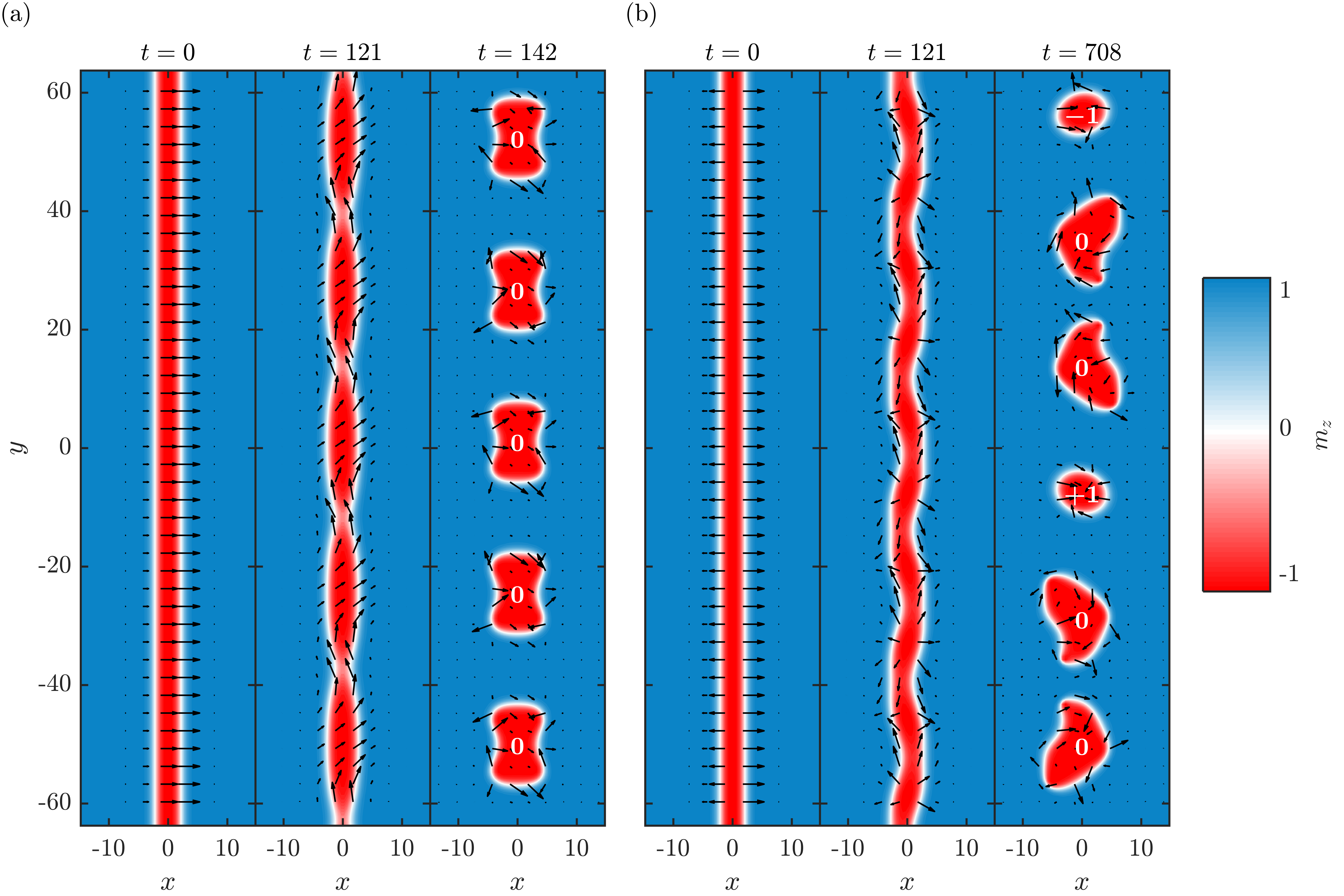
First, we consider the case of a non-topological bion stripe. The initial condition consists of the bion stripe (9) with its frequency modulated with . This represents a small perturbation of the non-topological bion stripe. The temporal evolution of the bion stripe is shown in Fig. 8(a). At , shown in the leftmost frame, the bion stripe is only slightly perturbed in the direction. As time evolves, the unstable mode grows and develops a symmetric, neck instability of the bion stripe width, visible in the central panel at and consistent with the linear stability analysis of Sec. III. The observed oscillation wavelength is 25.6, equal to the maximally unstable wavelength . Further evolution in time deviates from the linear regime and the bion filament pinches and is severed, leading to the formation of two-dimensional structures. We observe five structures that subsequently divide and merge in pairs, establishing breathers [29]. A snapshot is is shown in the rightmost frame at . By computing the skyrmion number Eq. (2) in an area that encloses each structure and satisfies at the boundaries, we find that the resulting structures are topologically trivial, indicating that these breathers are composed of two droplets.
Now we consider the topological bion stripe. In this case, the instability is favored by spatially modulating the bion’s offset where , . The temporal evolution of the topological bion filament is shown in Fig. 8(b). The leftmost frame shows the slightly perturbed initial state at . At time , shown in the central frame of Fig. 8(b), a snake instability is observed. Here, the instability is dominated by a modulation of the offset with wavelength but also exhibits a slight modulation in the width. As noted in the previous sections, this is caused by nonlinear coupling between the filament width and center that is disregarded in the linear stability analysis considered in Sec. III. Interestingly, the instability leads to the separation of topological poles and anti-poles marked by a positive or negative chirality, respectively. The time of the central frame is the same as that of the non-topological case, indicating that the growth rate is approximately independent of topology in agreement with Eq. (21). The poles and anti-poles eventually separate from the bion filament and shrink below the numerical grid scale, ultimately annihilating into a burst of spin wave radiation. The remains of the soliton filament establish two-dimensional textures, as shown in the rightmost frame of Fig. 8(b) at . The dynamic evolution from the bion filament separation to the (approximate) stabilization of two-dimensional textures includes annihilation of topological poles and merging of textures, requiring much longer times to stabilize. The resultant textures in this case include a skyrmion, an anti-skyrmion, and four droplets, conserving the system’s trivial skyrmion number.
The long time dynamics cannot be accurately predicted because of the interactions between the resulting two-dimensional structures after the bion filamentary breakup. However, the linear stability analysis can be used to predict the dynamics shortly after breakup and, consequently, the number of non-topological textures and topological poles that result from the instability. For the non-topological bion stripe, the filament is severed where the frequency approaches unity, i.e., a homogeneous, out-of-plane magnetization. This implies that the number of non-topological textures per unit length, , can be estimated as the inverse of the maximally unstable wavelength
| (26) |
For the parameters used in the numerical simulation, , so the total number of textures in a domain of height is predicted to be . Coincidentally, this agrees with the five breathers observed in Fig. 8(a) at long times after breakup, but we stress that each breather is composed of two droplets. For the topological bion, we can predict how topological poles form within the bion filament. The limit in the phase yields a phase jump for , as noted in Eq. (10). For small but nonzero , we have the expansion of Eq. (9b)
| (27) |
where . Equation (27) expresses the smoothing of the phase jump by a nonzero velocity . The phase jump is negative when and positive for . Therefore, when the velocity passes through zero with or , a topological pole is formed. The sign of the pole’s skyrmion number [recall Eq. (2)] is opposite the spatial slope of , i.e., . Because there are two velocity zero crossings per period of the instability, we can write the poles per unit length as
| (28) |
Note that this is simply twice Eq. (26).
VI Discussion: bion stripes in physically confined systems
The linear stability analysis presented in Sec. III predicts a long wavelength instability of bion stripes and provides quantitative information on the dynamics and nucleation of two-dimensional structures for extended thin films under the assumption of only a local dipole field. In the case of physically confined systems, i.e. nanowires, our approach also provides quantitative predictions for the stabilization of bion stripes based on the allowed wavelengths.
For a bion stripe confined in the direction, the analysis presented above holds insofar as the bion stripe is sufficiently localized within the nanowire. In other words, interactions between the bion stripe and the physical boundary must be avoided. If this condition is satisfied, bion stripes for an extended domain in the direction will be unstable to long wavelength perturbations and favor the growth of the maximally unstable mode as shown in Fig. 8. For a bion stripe confined along the direction with a free spin boundary condition (), the instability depends on the dimensionless width of the nanowire, . Linear stability analysis (Sec. III) predicts that a bion stripe will be stable for widths
| (29) |
independent of its topology. Bion stripes in wider wires are unstable and will separate into two-dimensional textures. The nanowire width dependency is inversely proportional to the (square root of the) bion stripe precessional frequency. This implies that static bion stripes or bound domain walls of either Bloch or Néel type () are always stable. However, perturbations from e.g., thermal fluctuations, can induce dynamics and modulations of the bion filament’s width and frequency. Assuming an initial bion stripe frequency of , bion stripes will be stable for nanowires narrower than .
Physical insight on these conditions can be gained by scaling both the bion stripe frequency and nanowire width to physical units by multiplying by and , respectively (recall the non-dimensionalization in Sec. II). For example, if we consider ultra-thin CoFeB used in Ref. 24 with kA/m and kJ/m3 while assuming nm (this parameter was not characterized in Ref. 24), we obtain a bion stripe precessional frequency of MHz and a maximum width for a stable bion stripe nm. If we consider Co/Ni multilayers utilized in Ref. 17 with kA/m, kJ/m3, and nm, we obtain a bion stripe precessional frequency of MHz and a maximum width for a stable bion stripe nm. These results are well within state-of-the-art patterning capabilities and suggest that it is possible to control the stability of non-topological and topological bion stripes and their breakup into an a-priori specified/designed number of droplets or topological poles, similar to the prescription of the number of vortices via transverse instability in atomic Bose-Einstein condensates [38]. In that case too, the complete stabilization of two-dimensional stripes in the form of dark solitons has been advocated by suppressing the infrared catastrophes associated with the transverse instability via increased confinement; see, e.g., Ref. 48 and references therein.
We emphasize that these results were obtained for a minimal model of a magnetic material with perpendicular magnetic anisotropy and local dipole field. This assumption is justified for ultra-thin films that can be fabricated with current deposition methods [24]. For relatively thick films, non-local dipole is expected to stabilize labyrinthine domains [5] and further studies are needed to investigate the dynamics of bion stripes.
VII Conclusions
The transverse instability of a bion stripe was studied utilizing the average Lagrangian method. This approach approximates the dynamics by a soliton filament with spatio-temporally varying parameters and complements other recent theoretical approaches to the study of soliton filaments and shells[44, 43]. The benefit of these approaches is a reduction in the dimensionality of the system. For soliton filaments in two-dimensions, their parameters are governed by a nonlinear system of partial differential equations in one space dimension (the transverse direction) and time. These equations enable an analytically tractable linear stability analysis but their nonlinear evolution also accurately describes the full soliton filament’s dynamics.
We found that the early stage of the transverse instability for bion stripes can be described by exponential temporal growth in either the filament’s phase/frequency (non-topological case) or center/velocity (topological case). We used this result to predict the most unstable wavelength, maximal growth rate, and the dynamical manifestation of the instability. For non-topological bion stripes, we observed a neck instability that leads to a pinching of the bion filament. For topological bion stripes, we observed a snake instability that leads to the appearance of topological poles. Our linear stability analysis also identifies the smallest unstable wavelength that predicts the resulting number of two-dimensional waveforms, as well as the complete stabilization of bion stripes in the case of sufficient transverse confinement.
Nonlinear evolution of the average Lagrangian modulation equations accurately predicts the unstable dynamics up to the severing of the bion filament. We find that the result of filamentary breakup also depends on topology. For a perturbed, non-topological bion stripe, the neck instability results in a series of two-dimensional localized droplet solitons whose number can be estimated at shortly after breakup by the most unstable wavelength from linear theory. The snake instability for the topological bion stripe results in a chain of topological poles that annihilate and leave behind solitonic skyrmions, anti-skyrmions, and droplets. The topology of the bion stripe is effectively transferred to a subset of the resultant two-dimensional localized textures. While the maximally unstable wavelength from linear theory predicts the number of topological poles, these poles are unstable and shrink to singularities that go beyond the continuum model used here. Further study of the dynamics of these topological poles in a semi-classical discrete spin lattice model may be warranted.
We note that both the bion stripes and two-dimensional textures obtained in this study do not require chiral fields from, e.g., Dzyaloshinskii-Moriya interaction (DMI) [49, 50]. Bion stripes are exact solutions of a conservative magnetic system with axial symmetry. However, DMI may be important to stabilize bion stripes in the presence of damping. While a study of transverse instabilities in the presence of damping and DMI is certainly worthwhile, we here focused on the leading energy terms that stabilize localized textures, namely, exchange (dispersion) and anisotropy (nonlinearity).
The average Lagrangian method applied to magnetization dynamics as presented here can be extended to include more physics and to shed light on the internal dynamics of droplets, skyrmions, and domain walls.
Acknowledgements.
E.I. acknowledges support from the Swedish Research Council, Reg. No. 637-2014-6863. M.A.H. partially supported by NSF CAREER DMS-1255422. M.E.R. partially supported by the National Science Foundation, DMS-1407340.Appendix A Average Lagrangian for bion stripe filaments
The purpose of the averaged Lagrangian approach is to reduce the dimensionality of a difficult problem, at the expense of obtaining only an approximate description of the dynamics[39]. There are two major steps to the approach. First, one must assume a form of the expected solution which only explicitly depends on one of the problem’s dimensions. In the case of bion stripes, we integrate over the moving coordinate and assume that the parameters of the bion stripe, , , , and , are all functions of both the transverse direction, , and time, . This assumed solution is then substituted into the Lagrangian, Eq. (7), to obtain the Lagrangian restricted to bion filaments
| (30) |
where is the Lagrangian density after substitution.
The second step of the averaged Lagrangian approach is to integrate Eq. (30) over . Due to the nature of the bion stripe solution (9), the integration can be carried out using the Cauchy residue theorem, taking advantage of a translation symmetry in the imaginary component of , which is shared by many terms in . While this integration is not theoretically difficult, the Lagrangian that is obtained from the process turns out to be complicated unless additional assumptions are made on the bion filament’s frequency and velocity . The obtained average Lagrangian is therefore asymptotically expanded assuming . The result, in scaled variables, is given in Eq. (12).
Appendix B Linearized Larmor torque equation about the bion stripe
Starting with the Larmor torque Eq. (3) and (4), we linearize about the bion stripe solution. We assume that the magnetization can be written as , where is obtained by substituting the bion stripe solution in Eqs. (9a) and (9b) into Eq. (5). We are interested in linearizing about the stationary bion stripe, however the topological bion exhibits a discontinuity at . Therefore, for numerical stability purposes, we will consider the parameter regime for the topological bion, which smooths the discontinuity at without drastically changing the dispersion relation. For the non-topological bion, we are free to assume .
Because we are interested in bion stripes with a finite velocity , we transform coordinates to a moving reference frame, . We can remove the explicit time dependence by applying a rotation matrix
| (31) |
to the magnetization vector, i.e., . The linearized equation for is found to be
| (32) |
By construction, is only a function of , so we may assume a linear wave solution in and
| (33) |
The substitution of Eq. (33) into Eq. (32) yields the eigenvalue problem
| (34) |
We solve Eq. (34) using a numerical eigenvalue solver. We discretize spatially over a domain using data points. This resolution is sufficient to resolve any near-singular behavior near the origin of the topological bion. We use second order central finite difference stencils to estimate the derivatives in . We impose Neumann boundary conditions on . The instability growth rate is and the maximally unstable wavelength is found by maximizing this function over using a numerical optimization method.
References
- [1] Mark J. Ablowitz and Harvey Segur, Solitons and the inverse scattering transform (SIAM, 1981).
- [2] L. F. Mollenauer and J. P. Gordon, Solitons in optical fibers: fundamentals and applications (Academic Press, New York, 2006).
- [3] R. S. Johnson, A modern introduction to the mathematical theory of water waves (Cambridge University Press, Cambridge, 1997).
- [4] P. Kevrekidis, D. Frantzeskakis, and R. Carretero-González, The Defocusing Nonlinear Schrödinger Equation (Society for Industrial and Applied Mathematics, Philadelphia, PA, 2015) http://epubs.siam.org/doi/pdf/10.1137/1.9781611973945 .
- [5] Alex Hubert and Rudolf Schäfer, Magnetic domains: the analysis of magnetic microstructures (Springer, 2009).
- [6] A. Bisig, L. Heyne, O. Boulle, and M. Klaui, “Tunable steady-state domain wall oscillator with perpendicular magnetic anisotropy,” Applied Physics Letters 95, 162504 (2009).
- [7] Riccardo Hertel, Wulf Wulfhekel, and Jürgen Kirschner, “Domain-wall induced phase shifts in spin waves,” Phys. Rev. Lett. 93, 257202 (2004).
- [8] P. Yan, X. S. Wang, and X. R. Wang, “All-magnonic spin-transfer torque and domain wall propagation,” Phys. Rev. Lett. 107, 177207 (2011).
- [9] D. A. Allwood, Gang Xiong, M. D. Cooke, C. C. Faulkner, D. Atkinson, N. Vernier, and R. P. Cowburn, “Submicrometer ferromagnetic not gate and shift register,” Science 296 (2002).
- [10] Stuart S. P. Parkin, Masamitsu Hayashi, and Luc Thomas, “Magnetic domain-wall racetrack memory,” Science 320, 190–194 (2008).
- [11] A.M. Kosevich, B.A. Ivanov, and A.S. Kovalev, “Magnetic solitons,” Physics Reports 194, 117 – 238 (1990).
- [12] Hans-Benjamin Braun, “Topological effects in nanomagnetism: from superparamagnetism to chiral quantum solitons,” Advances in Physics 61, 1–116 (2012).
- [13] D. Weller, A. Moser, L. Folks, M. E. Best, Wen Lee, M. F. Toney, M. Schwickert, J. U. Thiele, and M. F. Doerner, “High materials approach to 100 gbits/in2,” IEEE Transactions on Magnetics 36, 10–15 (2000).
- [14] P. Bruno and J. P. Renard, “Magnetic surface anisotropy of transition metal ultrathin films,” Applied Physics A: Materials Science & Processing 49, 499–506 (1989), 10.1007/BF00617016.
- [15] F.J.A. den Broeder, W. Hoving, and P.J.H. Bloemen, “Magnetic anisotropy of multilayers,” Journal of Magnetism and Magnetic Materials 93, 562 – 570 (1991).
- [16] M. A. Hoefer, T. J. Silva, and Mark W. Keller, “Theory for a dissipative droplet soliton excited by a spin torque nanocontact,” Phys. Rev. B 82, 054432 (2010).
- [17] S. M. Mohseni, S. R. Sani, J. Persson, T. N. Anh Nguyen, S. Chung, Ye. Pogoryelov, P. K. Muduli, E. Iacocca, A. Eklund, R. K. Dumas, S. Bonetti, A. Deac, M. A. Hoefer, and J. Åkerman, “Spin torque-generated magnetic droplet solitons,” Science 339, 1295–1298 (2013).
- [18] F. Macià, D. Backes, and A. Kent, “Stable magnetic droplet solitons in spin transfer nanocontacts,” Nature Nanotechnol. 9, 992 (2014).
- [19] S. Lendínez, N. Statuto, D. Backes, A. D. Kent, and F. Macià, “Observation of droplet soliton drift resonances in a spin-transfer-torque nanocontact to a ferromagnetic thin film,” Phys. Rev. B 92, 174426 (2015).
- [20] S. Chung, A. Eklund, E. Iacocca, S. M. Mohseni, S. R. Sani, L. Bookman, M. A. Hoefer, R. K. Dumas, and J. Åkerman, “Magnetic droplet nucleation boundary in orthogonal spin-torque nano-oscillators,” Nature Communications 7, 11209 (2016).
- [21] S. Mühlbauer, B. Binz, F. Jonietz, C. Pfleiderer, A. Rosch, A. Neubauer, R. Georgii, and P. Böni, “Skyrmion lattice in a chiral magnet,” Science 323, 915–919 (2009).
- [22] X. Z. Yu, Y. Onose, N. Kanazawa, J. H. Park, J. H. Han, Y. Matsui, N. Nagaosa, and Y. Tokura, “Real-space observation of a two-dimensional skyrmion crystal,” Nature 465, 901 – 904 (2010).
- [23] Wanjun Jiang, Pramey Upadhyaya, Wei Zhang, Guoqiang Yu, M. Benjamin Jungfleisch, Frank Y. Fradin, John E. Pearson, Yaroslav Tserkovnyak, Kang L. Wang, Olle Heinonen, Suzanne G. E. te Velthuis, and Axel Hoffmann, “Blowing magnetic skyrmion bubbles,” Science 349, 283 – 286 (2015).
- [24] Wanjun Jiang, Xichao Zhang, Guoqiang Yu, Wei Zhang, Xiao Wang, M. Benjamin Jungfleisch, John E. Pearson, Xuemei Cheng, Olle Heinonen, Kang L. Wang, Yan Zhou, Axel Hoffmann, and G. E. te Velthius, “Direct observation of the skyrmion hall effect,” Nature Physics 13 (2016).
- [25] S. A. Montoya, S. Couture, J. J. Chess, J. C. T. Lee, N. Kent, D. Henze, S. K. Sinha, M.-Y. Im, S. D. Kevan, P. Fischer, B. J. McMorran, V. Lomakin, S. Roy, and E. E. Fullerton, “Tailoring magnetic energies to form dipole skyrmions and skyrmion lattices,” Phys. Rev. B 95, 024415 (2017).
- [26] Y. Zhou, E. Iacocca, A. Awad, R.K. Dumas, H.B. Zhang, H. B. Braun, and J. Åkerman, “Dynamically stabilized magnetic skyrmions,” Nature Communications 6 (2015).
- [27] A. Fert, V. Cros, and J. Sampaio, “Skyrmions on the track,” Nature Nanotechnology 8, 152 – 156 (2013).
- [28] Xichao Zhang, Motohiko Ezawa, and Yan Zhou, “Magnetic skyrmion logic gates: conversion, duplication and merging of skyrmions,” Scientific reports 5 (2015).
- [29] M. D. Maiden, L. D. Bookman, and M. A. Hoefer, “Attraction, merger, reflection, and annihilation in magnetic droplet soliton scattering,” Phys. Rev. B 89, 180409 (2014).
- [30] Shi-Zeng Lin, Cristian D. Batista, and Avadh Saxena, “Internal modes of a skyrmion in the ferromagnetic state of chiral magnets,” Phys. Rev. B 89, 024415 (2014).
- [31] D. Xiao, V. Tiberkevich, Y. H. Liu, Y. W. Liu, S. M. Mohseni, S. Chung, M. Ahlberg, A. N. Slavin, J. Åkerman, and Yan Zhou, “Parametric autoexcitation of magnetic droplet soliton perimeter modes,” Phys. Rev. B 95, 024106 (2017).
- [32] Jun-Young Lee, Ki-Suk Lee, Sangkook Choi, Konstantin Y. Guslienko, and Sang-Koog Kim, “Dynamic transformations of the internal structure of a moving domain wall in magnetic nanostripes,” Phys. Rev. B 76, 184408 (2007).
- [33] Yoko Yoshimura, Kab-Jin Kim, Takuya Taniguchi, Takayuki Tono, Kohei Ueda, Ryo Hiramatsu, Takahiro Moriyama, Keisuke Yamada, Yoshinobu Nakatani, and Teruo Ono, “Soliton-like magnetic domain wall motion induced by the interfacial dzyaloshinskii-moriya interaction,” Nature Physics 12, 157 (2015).
- [34] Ezio Iacocca, Randy K. Dumas, Lake Bookman, Majid Mohseni, Sunjae Chung, Mark A. Hoefer, and Johan Åkerman, “Confined dissipative droplet solitons in spin-valve nanowires with perpendicular magnetic anisotropy,” Phys. Rev. Lett. 112, 047201 (2014).
- [35] Olle Heinonen, Wanjun Jiang, Hamoud Somaily, Suzanne G. E. te Velthuis, and Axel Hoffmann, “Generation of magnetic skyrmion bubbles by inhomogeneous spin hall currents,” Phys. Rev. B 93, 094407 (2016).
- [36] Shi-Zeng Lin, “Edge instability in a chiral stripe domain under an electric current and skyrmion generation,” Phys. Rev. B 94, 020402 (2016).
- [37] Yan Liu, Na Lei, Weisheng Zhao, Wenqing Liu, Antonio Ruotolo, Hans-Benjamin Braun, and Yan Zhou, “Chopping skyrmions from magnetic chiral domains with uniaxial stress in magnetic nanowire,” Applied Physics Letters 111, 022406 (2017).
- [38] Manjun Ma, R. Carretero-González, P. G. Kevrekidis, D. J. Frantzeskakis, and B. A. Malomed, “Controlling the transverse instability of dark solitons and nucleation of vortices by a potential barrier,” Phys. Rev. A 82, 023621 (2010).
- [39] B. A. Malomed, “Progress in optics,” (Elsevier, 2002) Chap. Variational methods in nonlinear fiber optics and related fields, pp. 69–191.
- [40] N. L. Schryer and L. R. Walker, “The motion of 180∘ domain walls in uniform dc magnetic fields,” Journal of Applied Physics 45, 5406–5421 (1974).
- [41] G. Chen, J. Zhu, A. Quesada, J. Li, A. T. N’Diaye, Y. Huo, T. P. Ma, Y. Chen, H. Y. Kwon, C. Won, Z. Q. Qiu, A. K. Schmid, and Y. Z. Wu, “Novel chiral magnetic domain wall structure in films,” Phys. Rev. Lett. 110, 177204 (2013).
- [42] Satoru Emori, Uwe Bauer, Sung-Min Ahn, Eduardo Martinez, and S. D. Beach, “Current-driven dynamics of chiral ferromagnetic domain walls,” Nature Materials. Advance online publication 12 (2013).
- [43] P. G. Kevrekidis, W. Wang, R. Carretero-Gonzalez, and D. J. Frantzeskakis, “Adiabatic invariant approach to transverse instability: Landau dynamics of soliton filaments,” Phys. Rev. Lett. 118, 244101 (2017).
- [44] V. A. Mironov, A. I. Smirnov, and L. A. Smirnov, “Dynamics of vortex structure formation during the evolution of modulation instability of dark solitons,” JETP 112, 46–59 (2011).
- [45] Dmitry V. Skryabin and William J. Firth, “Modulational instability of solitary waves in nondegenerate three-wave mixing: The role of phase symmetries,” Phys. Rev. Lett. 81, 3379–3382 (1998).
- [46] M. A. Hoefer and B. Ilan, “Onset of transverse instabilities of confined dark solitons,” Phys. Rev. A 94, 013609 (2016).
- [47] M. A. Hoefer and M. Sommacal, “Propagating two-dimensional magnetic droplets,” Physica D: Nonlinear Phenomena 241, 890 – 901 (2012).
- [48] P. G. Kevrekidis, G. Theocharis, D. J. Frantzeskakis, and A. Trombettoni, “Avoiding infrared catastrophes in trapped bose-einstein condensates,” Phys. Rev. A 70, 023602 (2004).
- [49] I. E. Dzyaloshinskii, “A thermodynamic theory of weak ferromagnetism of antiferromagnetics,” Journal of Physics and Chemistry of Solids 4, 241 – 255 (1958).
- [50] Tôru Moriya, “Anisotropic superexchange interaction and weak ferromagnetism,” Phys. Rev. 120, 91–98 (1960).