跳到论文正文
W Papers独立论文阅读器 arXiv:1710.07661 论文正文 计算阅读时间 · 0%
引用这篇论文根据当前论文元数据生成,正式投稿前建议核对。


License: arXiv.org perpetual non-exclusive license
arXiv:1710.07661v3 [math.NA] 02 Oct 2018

Finite element approximation of nonlocal fracture models

\shortauthorlist

Prashant K. Jha and Robert Lipton

Finite element approximation of nonlocal fracture models

Prashant K. Jha and Robert Lipton
Department of Mathematics, Louisiana State University,
Baton Rouge, LA, 70803
††thanks: Email: prashant.j16o@gmail.com, Orcid: https://orcid.org/0000-0003-2158-364X††thanks: Corresponding author. Email: lipton@math.lsu.edu, Orcid: https://orcid.org/0000-0002-1382-3204
Abstract

We consider nonlocal nonlinear potentials and estimate the rate of convergence of time stepping schemes to the peridynamic equation of motion. We begin by establishing the existence of H2H^{2} solutions over any finite time interval. Here spatial approximation by finite element interpolations are considered. The energy stability of the associated semi-discrete time stepping scheme is established and the approximation of strong and weak formulations of the evolution using FE interpolations of H2H^{2} solutions are investigated. The strong and weak form of approximations are shown to converge to the actual solution in the mean square norm at the rate Ct​Δ​t+Cs​h2/ϵ2C_{t}\Delta t+C_{s}h^{2}/\epsilon^{2} where hh is the mesh size, ϵ\epsilon is the size of nonlocal interaction and Δ​t\Delta t is the time step. The constants CtC_{t} and CsC_{s} are independent of Δ​t\Delta t, and hh. In the absence of nonlinearity a CFL like condition for the energy stability of the central difference time discretization scheme is developed. nonlocal fracture models; peridynamics; cohesive dynamics; numerical analysis; finite element method.

†† This material is based upon work supported by the U. S. Army Research Laboratory and the U. S. Army Research Office under contract/grant number W911NF1610456.

1 Introduction

In this article we consider non local models for crack propagation in solids. We focus on the peridynamics formulation introduced in Silling (2000). The basic idea is to redefine the strain in terms of the difference quotients of the displacement field and allow for nonlocal interaction within some finite horizon. The formulation has a natural length scale given by the size of the horizon. The force at any given material point is computed by considering the deformation of all neighboring material points within a radius given by the size of horizon. Here we examine the finite element approximation to the nonlinear nonlocal model proposed and examined in Lipton (2014); Lipton (2016). One of the important points of this model is the fact that as the size of the horizon goes to zero, i.e. when we tend to the local limit, the model behaves as if it is an elastic model away from the crack set and has bounded Griffith fracture energy Lipton (2014); Lipton (2016). Therefore, in the limit, the model not only converges to the local elastic models in regions with small deformation but also has finite Griffith fracture energy associated with a sharp fracture set. The nonlinear potential can be calibrated so that it gives the same fracture toughness as in Linear Elastic Fracture Mechanics models. The force potential used in this model is a smooth version of the prototypical micro elastic brittle model introduced in Silling (2000). Further, the slope of the nonlinear force for small strain (as we show in Section 2) is controlled by elastic constant of the material.

The linear peridynamic model converges to the linear elastic model, when the nonlocal length scale goes to zero, this is seen in the convergence of the integral operators to the differential operators, see Emmrich et al. (2013); Silling & Lehoucq (2008); Aksoylu & Unlu (2014). More fundamentally the convergence of linear peridynamics to local elasticity in the sense of solution operators is shown in Mengesha & Du (2015). Crack propagation using the peridynamics model has been considered extensively, see Silling et al. (2010); Bobaru & Hu (2012); Ha & Bobaru (2010); Agwai et al. (2011); Ghajari et al. (2014); Diehl et al. (2016); Lipton et al. (2016). Theoretical analysis of peridynamics models are carried out in Lipton (2014); Lipton (2016); Foster et al. (2011); Mengesha & Du (2013); Du & Zhou (2011); Emmrich et al. (2013); Aksoylu & Parks (2011); Dayal (2017) and Macek & Silling (2007); Littlewood (2010); Du et al. (2013); Gerstle et al. (2007). Dynamic phase transformations described by peridynamic theory has been proposed and analyzed in Dayal & Bhattacharya (2006).

In this work, we consider the finite element interpolation given by linear conforming elements. The potential considered in this work is of double well type. One well corresponds to linear elastic deformation and is zero for zero strain and other corresponds to material rupture and has a well at infinity. We consider discrete time stepping methods both in weak and strong form. To proceed we first show the existence of evolutions in H2​(D,𝐑d)∩H01​(D,𝐑d)H^{2}(D;\mathbf{R}^{d})\cap H^{1}_{0}(D;\mathbf{R}^{d}), see Theorem 3.2. Here the H2H^{2} norm for the evolution can become large as the length scale of nonlocal interaction becomes small. In Theorem 3.3, we show that the peridynamic evolution can have higher regularity in time when body forces satisfy additional regularity conditions in time. We next address the stability of semi-discrete approximation for the nonlinear model and show that the evolution is energetically stable, see Theorem 4.1. We then consider the linearization of the nonlinear model and provide a stability analysis of the fully discrete approximation. Here we folliw Karaa (2012) and Guan & Gunzburger (2015) to obtain a stability condition on Δ​t\Delta t for the linearized model, see Theorem 5.4. The rationale is that for small strains the material behaves like a linear elastic material. Recent related work for linear local elastic models establish stability of the general Newmark time discretization Baker (1976); Grote & Schötzau (2009); Karaa (2012). This behavior is shown to persist for elastic nonlocal models in Guan & Gunzburger (2015), using techniques in Baker (1976); Grote & Schötzau (2009); Karaa (2012). For the nonlinear model we establish a Lax Richtmyer stability, see Lemma 5.3 and \eqrefLaxRichtmyer.

The main contribution of this paper is the approximation of H2​(D,𝐑d)∩H01​(D,𝐑d)H^{2}(D;\mathbf{R}^{d})\cap H^{1}_{0}(D;\mathbf{R}^{d}) peridynamic evolutions by linear conforming elements. The time stepping approximation using finite element interpolation for both strong and weak forms of the evolution problem is shown to converge to the actual solution in the mean square norm at the rate Ct​Δ​t+Cs​h2/ϵ2C_{t}\Delta t+C_{s}h^{2}/\epsilon^{2} where hh is the mesh size, ϵ\epsilon is the size of nonlocal interaction and Δ​t\Delta t is the time step, see Theorem 5.1. The constant CtC_{t} is independent of Δ​t\Delta t and hh and depends on the L2L^{2} norm of the time derivatives of the exact solution. The constant CsC_{s} is also independent of Δ​t\Delta t, and hh and depends on the H2H^{2} norm of the exact solution. We assess the impact of the constants appearing in Theorem 5.1 for evolution times seen in fracture experiments in section 7. Related recent work, Jha & Lipton (2018a), addresses time stepping methods for the strong form approximation in Hölder space C0,γ​(D,𝐑d)C^{0,\gamma}(D;\mathbf{R}^{d}) with Hölder exponent γ∈(0,1]\gamma\in(0,1]. A convergence rate of Ct​Δ​t+Cs​hγ/ϵ2C_{t}\Delta t+C_{s}h^{\gamma}/\epsilon^{2} is demonstrated. The constant CtC_{t} depends on L2L^{2} norm of the time derivative of exact solution and the constant CsC_{s} depends on the Hölder norm of the exact solution and the Lipschitz constant of peridynamic force.

The organization of article is as follows: In Section 2, we introduce the class of nonlocal nonlinear potentials used in this article. We establish the existence of H2​(D,𝐑d)∩H01​(D,𝐑d)H^{2}(D;\mathbf{R}^{d})\cap H^{1}_{0}(D;\mathbf{R}^{d}) solutions in Section 3. In Section 4 we describe the finite element approximation and establish energy stability for the semi-discrete in time approximation. In Section 5 we consider the central in time discretization and describe the convergence rate of the FEM approximation to the true solution. We establish a CFL like criterion on the time step for stability of the linearized model. The proof of claims are given in Section 6. We discuss the convergence rate and the associated a-priori error over time scales seen in fracture experiments, see Section 7. We provide concluding remarks addressing the existence of asymptotically compatible schemes in the context of fracture, see Section 8.

2 Class of bond-based nonlinear potentials

In this section, we present the nonlinear nonlocal model. Let D⊂𝐑dD\subset\mathbf{R}^{d}, for d=2,3d=2,3 be the material domain with characteristic length-scale of unity. To fix ideas DD is assumed to be an open set with C1C^{1} boundary. Every material point x∈Dx\in D interacts nonlocally with all other material points inside a horizon of length ϵ∈(0,1)\epsilon\in(0,1). Let Hϵ​(x)H_{\epsilon}(x) be the ball of radius ϵ\epsilon centered at xx containing all points yy that interact with xx. After deformation the material point xx assumes position z=x+u⁡(x)z=x+u(x). In this treatment we assume infinitesimal displacements u⁡(x)u(x) so the deformed configuration is the same as the reference configuration and the linearized strain is given by {align*} S=S(y,x;u) = \dfracu(y) - u(x)—y - x— ⋅\dfracy - x—y - x—.

We let tt denote time and the displacement field u⁡(t,x)u(t,x) evolves according to Newton’s second law

ρ​∂t​t2u⁡(t,x)\displaystyle\rho\partial^{2}_{tt}u(t,x) =−∇PDϵ(u(t))(x)+b(t,x)\displaystyle=-\nabla PD^{\epsilon}(u(t))(x)+b(t,x) (1)

for all x∈Dx\in D. Here the body force applied to the domain DD can evolve with time and is denoted by b⁡(t,x)b(t,x). Without loss of generality, we will assume ρ=1\rho=1. The peridynamic force denoted by −∇PDϵ(u)(x)-\nabla PD^{\epsilon}(u)(x) is given by summing up all forces acting on xx,

−∇PDϵ(u)(x)=2ϵd​ωd∫Hϵ​(x)∂SWϵ(S,y−x)y−x|y−x|dy,\displaystyle-\nabla PD^{\epsilon}(u)(x)=\dfrac{2}{\epsilon^{d}\omega_{d}}\int_{H_{\epsilon}(x)}\partial_{S}W^{\epsilon}(S,y-x)\dfrac{y-x}{|y-x|}dy,

where ∂SWϵ\partial_{S}W^{\epsilon} is the force exerted on xx by yy and is given by the derivative of the nonlocal two point potential Wϵ​(S,y−x)W^{\epsilon}(S,y-x) with respect to the strain and ωd\omega_{d} is volume of unit ball in dimension dd.

Let ∂D\partial D be the boundary of material domain DD. The Dirichlet boundary condition on uu is

u⁡(t,x)=0∀x∈∂D,∀t∈[0,T]\displaystyle u(t,x)=0\qquad\forall x\in\partial D,\forall t\in[0,T] (2)

and the initial condition is

u⁡(0,x)=u0​(x)and∂tu⁡(0,x)=v0​(x).\displaystyle u(0,x)=u_{0}(x)\qquad\text{and}\qquad\partial_{t}u(0,x)=v_{0}(x). (3)

The initial data and solution u⁡(t,x)u(t,x) are extended by 00 outside DD. We remark that traction boundary conditions can be introduced in the nonlocal context by prescribing a body force along a boundary layer of width ϵ\epsilon and allowing the displacement to be free there.

Define the energy ℰϵ​(u)​(t)\mathcal{E}^{\epsilon}(u)(t) to be the sum of kinetic and potential energy and is given by

ℰϵ​(u)​(t)\displaystyle\mathcal{E}^{\epsilon}(u)(t) =12​‖u˙​(t)‖L2+P​Dϵ​(u⁡(t)).\displaystyle=\frac{1}{2}||\dot{u}(t)||_{L^{2}}+PD^{\epsilon}(u(t)). (4)

where potential energy P​DϵPD^{\epsilon} is given by

P​Dϵ​(u)\displaystyle PD^{\epsilon}(u) =∫D[1ϵd​ωd​∫Hϵ​(x)|y−x|​Wϵ​(S⁡(u),y−x)​𝑑y]​𝑑x.\displaystyle=\int_{D}\left[\dfrac{1}{\epsilon^{d}\omega_{d}}\int_{H_{\epsilon}(x)}|y-x|W^{\epsilon}(S(u),y-x)dy\right]dx.

2.1 Nonlocal potential

We now describe the nonlocal potential. We consider potentials WϵW^{\epsilon} of the form

Wϵ​(S,y−x)\displaystyle W^{\epsilon}(S,y-x) =ω⁡(x)​ω​(y)​Jϵ​(|y−x|)ϵ​|y−x|​f​(|y−x|​S2),\displaystyle=\omega(x)\omega(y)\dfrac{J^{\epsilon}(|y-x|)}{\epsilon|y-x|}f(|y-x|S^{2}), (5)

where f:𝐑+→𝐑f:\mathbf{R}^{+}\to\mathbf{R} is assumed to be positive, smooth, and concave with following properties

limr→0+f⁡(r)r=f′​(0),limr→∞f⁡(r)=f∞<∞.\displaystyle\lim_{r\to 0^{+}}\dfrac{f(r)}{r}=f^{\prime}(0),\qquad\lim_{r\to\infty}f(r)=f_{\infty}<\infty. (6)

The peridynamic force −∇PDϵ-\nabla PD^{\epsilon} is written as

−∇PDϵ(u)(x)=4ϵd+1​ωd∫Hϵ​(x)ω(x)ω(y)Jϵ(|y−x|)f′(|y−x|S(u)2)S(u)ey−xdy,\displaystyle-\nabla PD^{\epsilon}(u)(x)=\dfrac{4}{\epsilon^{d+1}\omega_{d}}\int_{H_{\epsilon}(x)}\omega(x)\omega(y)J^{\epsilon}(|y-x|)f^{\prime}(|y-x|S(u)^{2})S(u)e_{y-x}dy, (7)

where we used the notation S⁡(u)=S⁡(y,x,u)S(u)=S(y,x;u) and ey−x=y−x|y−x|e_{y-x}=\frac{y-x}{|y-x|}.

The function Jϵ​(|y−x|)J^{\epsilon}(|y-x|) models the influence of separation between points yy and xx. Here Jϵ​(|y−x|)=J⁡(|y−x|/ϵ)J^{\epsilon}(|y-x|)=J(|y-x|/\epsilon) can be piecewise smooth and we define JJ to be zero outside the ball {ξ:|ξ|<1}=H1​(0)\{\xi:\,|\xi|<1\}=H_{1}(0) and 0≤J⁡(|ξ|)≤M0\leq J(|\xi|)\leq M for all ξ∈H1​(0)\xi\in H_{1}(0).

The boundary function ω⁡(x)\omega(x) is nonnegative and takes the value 11 for points xx inside DD of distance ϵ\epsilon away from from the boundary ∂D\partial D. Inside the boundary layer of width ϵ\epsilon the function ω⁡(x)\omega(x) smoothly decreases from 11 to 00 taking the value 00 on ∂D\partial D.

In the sequel we will set

ω¯ξ​(x)=ω⁡(x)​ω​(x+ϵ​ξ)\displaystyle\bar{\omega}_{\xi}(x)=\omega(x)\omega(x+\epsilon\xi) (8)

and we assume

|∇ω¯ξ|≤Cω1<∞and|∇2ω¯ξ|≤Cω2<∞.\displaystyle|\nabla\bar{\omega}_{\xi}|\leq C_{\omega_{1}}<\infty\quad\text{and}\quad|\nabla^{2}\bar{\omega}_{\xi}|\leq C_{\omega_{2}}<\infty.

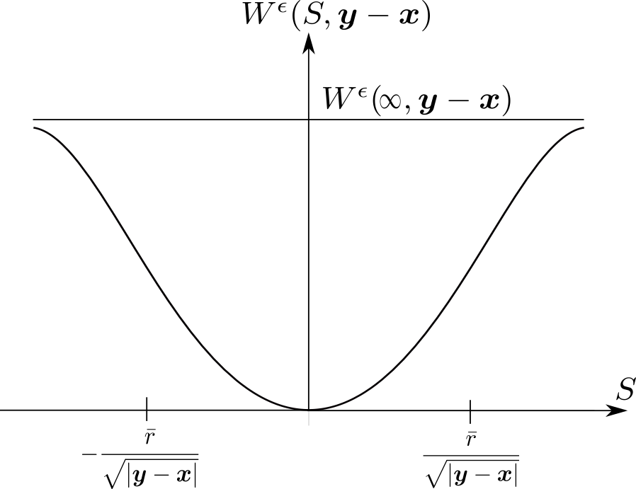
The potential described in (5) gives the convex-concave dependence, see Fig 1, of W⁡(S,y−x)W(S,y-x) on the strain SS for fixed y−xy-x. Initially the deformation is elastic for small strains and then softens as the strain becomes larger. The critical strain where the force between xx and yy begins to soften is given by Sc​(y,x):=r¯/|y−x|S_{c}(y,x):=\bar{r}/\sqrt{|y-x|} and the force decreases monotonically for

|S⁡(y,x,u)|>Sc.\displaystyle|S(y,x;u)|>S_{c}. (9)

Here r¯\bar{r} is the inflection point of r↦f⁡(r2)r\mapsto f(r^{2}) and is the root of following equation

f′​(r2)+2​r2​f′′​(r2)=0.\displaystyle f^{\prime}({r}^{2})+2{r}^{2}f^{\prime\prime}({r}^{2})=0. (10)
Refer to caption
Figure 1: Two-point potential Wϵ​(S,y−x)W^{\epsilon}(S,y-x) as a function of strain SS for fixed y−xy-x.
Refer to caption
Figure 2: Nonlocal force ∂SWϵ​(S,y−x)\partial_{S}W^{\epsilon}(S,y-x) as a function of strain SS for fixed y−xy-x. Second derivative of Wϵ​(S,y−x)W^{\epsilon}(S,y-x) is zero at ±r¯/|y−x|\pm\bar{r}/\sqrt{|y-x|}.

In [Theorem 5.2, Lipton (2016)], it is shown that in the limit ϵ→0\epsilon\to 0, the peridynamics solution has bounded linear elastic fracture energy, provided the initial data (u0,v0)(u_{0},v_{0}) has bounded linear elastic fracture energy and u0u_{0} is bounded. The elastic constant (Lamé constant λ\lambda and μ\mu) and energy release rate of the limiting energy is given by

λ=μ=Cd​f′​(0)​Md,𝒢c=2​ωd−1ωd​f∞​Md\displaystyle\lambda=\mu=C_{d}f^{\prime}(0)M_{d},\quad\mathcal{G}_{c}=\dfrac{2\omega_{d-1}}{\omega_{d}}f_{\infty}M_{d}

where Md=∫01J⁡(r)​rd​𝑑rM_{d}=\int_{0}^{1}J(r)r^{d}dr and f∞=limr→∞f⁡(r)f_{\infty}=\lim_{r\to\infty}f(r). Cd=2/3,1/4,1/5C_{d}=2/3,1/4,1/5 for d=1,2,3d=1,2,3 respectively and ωn=1,2,π,4​π/3\omega_{n}=1,2,\pi,4\pi/3 for n=0,1,2,3n=0,1,2,3. Therefore, f′​(0)f^{\prime}(0) and f∞f_{\infty} are determined by the Lamé constant λ\lambda and fracture toughness 𝒢c\mathcal{G}_{c}.

2.2 Weak formulation

We now give the weak formulation of the evolution. Here the notation ||⋅||||\cdot|| denotes the L2L^{2} norm on DD, ||⋅||∞||\cdot||_{\infty} is used for the L∞L^{\infty} norm on DD, and ||⋅||n||\cdot||_{n} for Sobolev HnH^{n} norms on DD for n=1,2n=1,2. We denote the dot product in L2​(D,𝐑d)L^{2}(D;\mathbf{R}^{d}) by (⋅,⋅)(\cdot,\cdot). For n=1,2n=1,2 we recall that the Sobolev space H0n​(D,𝐑d)H^{n}_{0}(D;\mathbf{R}^{d}) is given by the closure in the HnH^{n} norm of the functions that are infinitely differentiable with compact support in DD. Multiplying (1) by a test function in u~\tilde{u} in H01​(D,𝐑d)H^{1}_{0}(D;\mathbf{R}^{d}) we get

(u¨​(t),u~)\displaystyle(\ddot{u}(t),\tilde{u}) =(−∇PDϵ(u(t)),u~)+(b(t),u~).\displaystyle=(-\nabla PD^{\epsilon}(u(t)),\tilde{u})+(b(t),\tilde{u}).

An integration by parts easily shows for all u,vu,v in H01​(D,𝐑d)H^{1}_{0}(D;\mathbf{R}^{d}) that

(−∇PDϵ(u),v)\displaystyle(-\nabla PD^{\epsilon}(u),v) =−aϵ​(u,v),\displaystyle=-a^{\epsilon}(u,v),

where

aϵ​(u,v)\displaystyle a^{\epsilon}(u,v) =2ϵd+1​ωd​∫D∫Hϵ​(x)ω⁡(x)​ω​(y)​Jϵ​(|y−x|)​f′​(|y−x|​S​(u)2)|y−x|S⁡(u)​S​(v)​𝑑y​𝑑x.\displaystyle=\dfrac{2}{\epsilon^{d+1}\omega_{d}}\int_{D}\int_{H_{\epsilon}(x)}\omega(x)\omega(y)J^{\epsilon}(|y-x|)f^{\prime}(|y-x|S(u)^{2})|y-x|S(u)S(v)dydx. (11)

The same identities hold for all functions in L2​(D,𝐑d)L^{2}(D;\mathbf{R}^{d}).

It is readily verified that the peridynamic force and energy are bounded for all functions in L2​(D,𝐑d)L^{2}(D;\mathbf{R}^{d}). Here the bound on the force follows from the Lipschitz property of the force in L2​(D,𝐑d)L^{2}(D;\mathbf{R}^{d}), see, (22). The peridynamic force is also bounded for functions uu in H1​(D,𝐑d)H^{1}(D;\mathbf{R}^{d}). This again follows from the Lipschitz property of the force in H1​(D,𝐑d)H^{1}(D;\mathbf{R}^{d}) using arguments established in section 6. The boundedness of the energy P​Dϵ​(u)PD^{\epsilon}(u) in both L2​(D,𝐑d)L^{2}(D;\mathbf{R}^{d}) and H1​(D,𝐑d)H^{1}(D;\mathbf{R}^{d}) follows from the boundedness of the bond potential energy Wϵ​(S⁡(u),y−x){W}^{\epsilon}(S(u),y-x) used in the definition of P​Dϵ​(u)PD^{\epsilon}(u), see (5). More generally this also shows that P​Dϵ​(u)<∞PD^{\epsilon}(u)<\infty for u∈L1​(D,𝐑d)u\in L^{1}(D;\mathbf{R}^{d}).

Finally, the weak form of the evolution in terms of the operator aϵa^{\epsilon} becomes

(u¨​(t),u~)+aϵ​(u⁡(t),u~)\displaystyle(\ddot{u}(t),\tilde{u})+a^{\epsilon}(u(t),\tilde{u}) =(b⁡(t),u~).\displaystyle=(b(t),\tilde{u}). (12)

Using definition of aϵa^{\epsilon} in (11), one easily sees that

dd​t​ℰϵ​(u)​(t)=(u¨​(t),u˙​(t))+aϵ​(u⁡(t),u˙​(t)).\displaystyle\dfrac{d}{dt}\mathcal{E}^{\epsilon}(u)(t)=(\ddot{u}(t),\dot{u}(t))+a^{\epsilon}(u(t),\dot{u}(t)). (13)

3 Existence of solutions in H2∩H01H^{2}\cap H^{1}_{0}

We consider function space WW given by

W:=H2(D;𝐑d)∩H01(D;𝐑d)={v∈H2(D;𝐑d):γv=0,on ∂D},\displaystyle W:=H^{2}(D;\mathbf{R}^{d})\cap H^{1}_{0}(D;\mathbf{R}^{d})=\{v\in H^{2}(D;\mathbf{R}^{d}):\gamma v=0,\>\text{on }\partial D\}, (14)

where γ​v\gamma v is the trace of function vv on the boundary ∂D\partial D. Norm on WW is H2​(D,𝐑d)H^{2}(D;\mathbf{R}^{d}) norm. In this section, we show that for suitable initial condition and body force solutions of peridynamic equation exist in WW. We will assume that u∈Wu\in W is extended by zero outside DD.

We note the following Sobolev embedding properties of H2​(D,𝐑d)H^{2}(D;\mathbf{R}^{d}) when DD is a C1C^{1} domain.

  • •

    From Theorem 2.72 of Demengel & Demengel (2012), there exists a constant Ce1C_{e_{1}} independent of u∈H2​(D,𝐑d)u\in H^{2}(D;\mathbf{R}^{d}) such that

    ‖u‖L∞​(D,𝐑d)≤Ce1​‖u‖H2​(D,𝐑d).\displaystyle||u||_{L^{\infty}(D;\mathbf{R}^{d})}\leq C_{e_{1}}||u||_{H^{2}(D;\mathbf{R}^{d})}. (15)
  • •

    Further application of standard embedding theorems (e.g., Theorem 2.72 of Demengel & Demengel (2012)), shows there exists a constant Ce2C_{e_{2}} independent of uu such that

    ‖∇u‖Lq​(D,𝐑d×d)≤Ce2​‖∇u‖H1​(D,𝐑d×d)≤Ce2||u||H2​(D,𝐑d),\displaystyle||\nabla u||_{L^{q}(D;\mathbf{R}^{d\times d})}\leq C_{e_{2}}||\nabla u||_{H^{1}(D;\mathbf{R}^{d\times d})}\leq C_{e_{2}}||u||_{H^{2}(D;\mathbf{R}^{d})}, (16)

    for any qq such that 2≤q<∞2\leq q<\infty when d=2d=2 and 2≤q≤62\leq q\leq 6 when d=3d=3.

In what follows, we first state the Lipschitz continuity property for −∇PDϵ(u)-\nabla PD^{\epsilon}(u). We then state the existence theorem for solutions over finite time intervals. These are proved in section 6. We now write the peridynamic evolution equation as an equivalent first order system with y1​(t)=u​(t)y_{1}(t)=u(t) and y2​(t)=v​(t)y_{2}(t)=v(t) with v​(t)=u˙​(t)v(t)=\dot{u}(t). Let y=(y1,y2)Ty=(y_{1},y_{2})^{T} where y1,y2∈Wy_{1},y_{2}\in W and let Fϵ​(y,t)=(F1ϵ​(y,t),F2ϵ​(y,t))TF^{\epsilon}(y,t)=(F^{\epsilon}_{1}(y,t),F^{\epsilon}_{2}(y,t))^{T} such that

F1ϵ​(y,t)\displaystyle F^{\epsilon}_{1}(y,t) :=y2,\displaystyle:=y_{2}, (17)
F2ϵ​(y,t)\displaystyle F^{\epsilon}_{2}(y,t) :=−∇PDϵ(y1)+b(t).\displaystyle:=-\nabla PD^{\epsilon}(y_{1})+b(t). (18)

The initial boundary value is equivalent to the initial boundary value problem for the first order system given by

y˙​(t)=Fϵ​(y,t),\displaystyle\dot{y}(t)=F^{\epsilon}(y,t), (19)

with initial condition given by y⁡(0)=(u0,v0)T∈W×Wy(0)=(u_{0},v_{0})^{T}\in W\times W. Recall that we denote the norm on H2​(D,𝐑d)H^{2}(D;\mathbf{R}^{d}) as ||⋅||2||\cdot||_{2}.

Theorem 3.1.

Lipschitz continuity of the peridynamic force
For any u,v∈Wu,v\in W, we have

||−∇PDϵ(u)−(−∇PDϵ(v))||2\displaystyle||-\nabla PD^{\epsilon}(u)-(-\nabla PD^{\epsilon}(v))||_{2}
≤L¯1+L¯2​(‖u‖2+||v||2)+L¯3​(‖u‖2+||v||2)2ϵ3​‖u−v‖2\displaystyle\leq\dfrac{\bar{L}_{1}+\bar{L}_{2}(||u||_{2}+||v||_{2})+\bar{L}_{3}(||u||_{2}+||v||_{2})^{2}}{\epsilon^{3}}||u-v||_{2} (20)

where constants L¯1,L¯2,L¯3\bar{L}_{1},\bar{L}_{2},\bar{L}_{3} are independent of ϵ\epsilon, uu, and vv, and are defined in (116). Also, for u∈Wu\in W, we have

||−∇PDϵ(u)||2\displaystyle||-\nabla PD^{\epsilon}(u)||_{2} ≤L¯4​‖u‖2+L¯5​‖u‖22ϵ5/2,\displaystyle\leq\dfrac{\bar{L}_{4}||u||_{2}+\bar{L}_{5}||u||^{2}_{2}}{\epsilon^{5/2}}, (21)

where constants are independent of ϵ\epsilon and uu and are defined in (125).

In Theorem 6.1 of Lipton (2016), the Lipschitz property of the peridynamic force is shown in L2​(D,𝐑d)L^{2}(D;\mathbf{R}^{d}) and is given by

∥−∇PDϵ(u)−(−∇PDϵ(v))∥\displaystyle\|{-\nabla PD^{\epsilon}(u)-(-\nabla PD^{\epsilon}(v))}\| ≤L1ϵ2​‖u−v‖​∀u,v∈L2​(D,𝐑d),\displaystyle\leq\dfrac{L_{1}}{\epsilon^{2}}\|{u-v}\|\,\,\,\,\,\forall u,v\in L^{2}(D;\mathbf{R}^{d}), (22)

with L1L_{1} given by (87).

We state the theorem which shows the existence and uniqueness of solution in any given finite time interval I0=(−T,T)I_{0}=(-T,T).

Theorem 3.2.

Existence and uniqueness of solutions over finite time intervals
For any initial condition x0∈X=W×Wx_{0}\in X=W\times W, time interval I0=(−T,T)I_{0}=(-T,T), and right hand side b⁡(t)b(t) continuous in time for t∈I0t\in I_{0} such that b⁡(t)b(t) satisfies supt∈I0‖b⁡(t)‖2<∞\sup_{t\in I_{0}}||b(t)||_{2}<\infty, there is a unique solution y⁡(t)∈C1​(I0,X)y(t)\in C^{1}(I_{0};X) of

y⁡(t)=x0+∫0tFϵ​(y⁡(τ),τ)​𝑑τ,y(t)=x_{0}+\int_{0}^{t}F^{\epsilon}(y(\tau),\tau)\,d\tau,

or equivalently

y′​(t)=Fϵ​(y⁡(t),t),with y⁡(0)=x0,y^{\prime}(t)=F^{\epsilon}(y(t),t),\hbox{with $y(0)=x_{0}$},

where y⁡(t)y(t) and y′​(t)y^{\prime}(t) are Lipschitz continuous in time for t∈I0t\in I_{0}.

It is found that the peridynamic evolutions have higher regularity in time for body forces that are differentiable in time. We now state the higher temporal regularity for peridynamic evolutions.

Theorem 3.3.

Higher regularity
Suppose the initial data and righthand side b⁡(t)b(t) satisfy the hypothesis of Theorem 3.2 and suppose further that b˙​(t)\dot{b}(t) exists and is continuous in time for t∈I0t\in I_{0} and supt∈I0‖b˙​(t)‖2<∞\sup_{t\in I_{0}}||\dot{b}(t)||_{2}<\infty. Then u∈C3​(I0,W)u\in C^{3}(I_{0};W) and

‖∂t​t​t3u⁡(t,x)‖2\displaystyle||\partial^{3}_{ttt}u(t,x)||_{2} ≤C⁡(1+sups∈I0‖u⁡(s)‖2+sups∈I0‖u⁡(s)‖22)ϵ3​sups∈I0‖∂tu⁡(s)‖2+‖b˙​(t,x)‖2,\displaystyle\leq\dfrac{C(1+\sup_{s\in I_{0}}||u(s)||_{2}+\sup_{s\in I_{0}}||u(s)||^{2}_{2})}{\epsilon^{3}}\sup_{s\in I_{0}}||\partial_{t}u(s)||_{2}+||\dot{b}(t,x)||_{2}, (23)

where CC is a positive constant independent of uu.

The proofs of Theorems 3.1, 3.2, and 3.3 are given in Section 6. We now discuss the finite element approximation of the peridynamic evolution.

4 Finite element interpolation

Let VhV_{h} be given by linear continuous interpolations over tetrahedral or triangular elements 𝒯h\mathcal{T}_{h} where hh denotes the size of finite element mesh. Here we assume the elements are conforming and the finite element mesh is shape regular and Vh⊂H01​(D,𝐑d)V_{h}\subset H^{1}_{0}(D;\mathbf{R}^{d}).

For a continuous function uu on D¯\bar{D}, ℐh​(u)\mathcal{I}_{h}(u) is the continuous piecewise linear interpolant on 𝒯h\mathcal{T}_{h}. It is given by

ℐh​(u)|T=ℐT​(u)∀T∈𝒯h,\displaystyle\mathcal{I}_{h}(u)\bigg|_{T}=\mathcal{I}_{T}(u)\qquad\forall T\in\mathcal{T}_{h}, (24)

where ℐT​(u)\mathcal{I}_{T}(u) is the local interpolant defined over finite element TT and is given by

ℐT​(u)=∑i=1nu⁡(xi)​ϕi.\displaystyle\mathcal{I}_{T}(u)=\sum_{i=1}^{n}u(x_{i})\phi_{i}. (25)

Here nn is the number of vertices in an element TT, xix_{i} is the position of vertex ii, and ϕi\phi_{i} is the linear interpolant associated to vertex ii.

Application of Theorem 4.4.20 and remark 4.4.27 in Brenner & Scott (2008) gives

||u−ℐh(u)||≤ch2||u||2, ∀u∈W.\displaystyle||u-\mathcal{I}_{h}(u)||\leq ch^{2}||u||_{2},\hbox{ }\qquad\forall u\in W. (26)

Let rh​(u)r_{h}(u) denote the projection of u∈Wu\in W on VhV_{h}. For the L2L^{2} norm it is defined as

‖u−rh​(u)‖\displaystyle||u-r_{h}(u)|| =infu~∈Vh‖u−u~‖.\displaystyle=\inf_{\tilde{u}\in V_{h}}||u-\tilde{u}||. (27)

and satisfies

(rh​(u),u~)=(u,u~),∀u~∈Vh.\displaystyle(r_{h}(u),\tilde{u})=(u,\tilde{u}),\qquad\forall\tilde{u}\in V_{h}. (28)

Since ℐh​(u)∈Vh\mathcal{I}_{h}(u)\in V_{h}, and (26) we see that

||u−rh(u)||≤ch2||u||2, ∀u∈W.\displaystyle||u-r_{h}(u)||\leq ch^{2}||u||_{2},\hbox{ }\qquad\forall u\in W. (29)

4.1 Semi-discrete approximation

Let uh​(t)∈Vhu_{h}(t)\in V_{h} be the approximation of u⁡(t)u(t) which satisfies the following

(u¨h​(t),u~)+aϵ​(uh​(t),u~)\displaystyle(\ddot{u}_{h}(t),\tilde{u})+a^{\epsilon}(u_{h}(t),\tilde{u}) =(b⁡(t),u~),∀u~∈Vh,.\displaystyle=(b(t),\tilde{u}),\qquad\forall\tilde{u}\in V_{h},. (30)

We now show that the semi-discrete approximation is stable, i.e. the energy at time tt is bounded by the initial energy and work done by the body force.

Theorem 4.1.

Energy stability of the semi-discrete approximation
The semi-discrete scheme is energetically stable and the energy ℰϵ​(uh)​(t)\mathcal{E}^{\epsilon}(u_{h})(t), defined in (4), satisfies the following bound

ℰϵ​(uh)​(t)\displaystyle\mathcal{E}^{\epsilon}(u_{h})(t) ≤[ℰϵ​(uh)​(0)+∫0t‖b⁡(τ)‖​𝑑τ]2.\displaystyle\leq\left[\sqrt{\mathcal{E}^{\epsilon}(u_{h})(0)}+\int_{0}^{t}||b(\tau)||d\tau\right]^{2}.
Proof 4.2.

Letting u~=u˙h​(t)\tilde{u}=\dot{u}_{h}(t) in (30) and applying the identity (13), we get

dd​t​ℰϵ​(uh)​(t)=(b⁡(t),u˙h​(t))≤‖b⁡(t)‖​‖u˙h​(t)‖.\displaystyle\dfrac{d}{dt}\mathcal{E}^{\epsilon}(u_{h})(t)=(b(t),\dot{u}_{h}(t))\leq||b(t)||\;||\dot{u}_{h}(t)||.

We also have

‖u˙h​(t)‖≤2​12​‖u˙h‖2+P​Dϵ​(uh​(t))=2​ℰϵ​(uh)​(t)\displaystyle||\dot{u}_{h}(t)||\leq 2\sqrt{\frac{1}{2}||\dot{u}_{h}||^{2}+PD^{\epsilon}(u_{h}(t))}=2\sqrt{\mathcal{E}^{\epsilon}(u_{h})(t)}

where we used the fact that P​Dϵ​(u)​(t)PD^{\epsilon}(u)(t) is nonnegative and

dd​t​ℰϵ​(uh)​(t)\displaystyle\dfrac{d}{dt}\mathcal{E}^{\epsilon}(u_{h})(t) ≤2​ℰϵ​(uh)​(t)​‖b⁡(t)‖.\displaystyle\leq 2\sqrt{\mathcal{E}^{\epsilon}(u_{h})(t)}\;||b(t)||.

Fix δ>0\delta>0 and let A⁡(t)=ℰϵ​(uh​(t))+δA(t)=\mathcal{E}^{\epsilon}(u_{h}(t))+\delta. Then from the equation above we easily see that

dd​t​A​(t)\displaystyle\dfrac{d}{dt}A(t) ≤2A⁡(t)||b(t)||⇒12dd​t​A​(t)A⁡(t)≤||b(t)||.\displaystyle\leq 2\sqrt{A(t)}\;||b(t)||\quad\Rightarrow\dfrac{1}{2}\dfrac{\frac{d}{dt}A(t)}{\sqrt{A(t)}}\leq||b(t)||.

Noting that 1a⁡(t)​d​a​(t)d​t=2​dd​t​a⁡(t)\frac{1}{\sqrt{a(t)}}\frac{da(t)}{dt}=2\frac{d}{dt}\sqrt{a(t)}, integrating from t=0t=0 to τ\tau and relabeling τ\tau as tt, we get

A⁡(t)\displaystyle\sqrt{A(t)} ≤A⁡(0)+∫0t‖b⁡(s)‖​𝑑s.\displaystyle\leq\sqrt{A(0)}+\int_{0}^{t}||b(s)||ds.

Letting δ→0\delta\to 0 and taking the square of both side proves the claim.

5 Central difference time discretization

For illustration, we consider the central difference scheme and present the convergence rate for the central difference scheme for the fully nonlinear problem. We point out that the extension of these results to the general Newmark scheme is straight forward. We conclude by considering a linearized peridynamic evolution and demonstrate CFL like conditions for stability of the fully discrete scheme.

Let Δ​t\Delta t be the time step. The exact solution at tk=k​Δ​tt^{k}=k\Delta t (or time step kk) is denoted as (uk,vk)(u^{k},v^{k}), with vk=∂uk/∂tv^{k}=\partial u^{k}/\partial t, and the projection onto VhV_{h} at tkt^{k} is given by (rh​(uk),rh​(vk))(r_{h}(u^{k}),r_{h}(v^{k})). The solution of the discrete problem at time step kk is denoted as (uhk,vhk)(u^{k}_{h},v^{k}_{h}).

We first describe the discrete approximation of the weak formulation of the peridynamic evolution. The initial data for displacement u0u_{0} and velocity v0v_{0} are approximated by their projections rh​(u0)r_{h}(u_{0}) and rh​(v0)r_{h}(v_{0}). Let uh0=rh​(u0)u^{0}_{h}=r_{h}(u_{0}) and vh0=rh​(v0)v^{0}_{h}=r_{h}(v_{0}). The discrete weak formulation of the peridynamic evolution is given as follows. For k≥1k\geq 1, (uhk,vhk)(u^{k}_{h},v^{k}_{h}) satisfies, for all u~∈Vh\tilde{u}\in V_{h},

(uhk+1−uhkΔ​t,u~)\displaystyle\left(\dfrac{u^{k+1}_{h}-u^{k}_{h}}{\Delta t},\tilde{u}\right) =(vhk+1,u~),\displaystyle=(v^{k+1}_{h},\tilde{u}),
(vhk+1−vhkΔ​t,u~)\displaystyle\left(\dfrac{v^{k+1}_{h}-v^{k}_{h}}{\Delta t},\tilde{u}\right) =(−∇PDϵ(uhk),u~)+(bhk,u~),\displaystyle=(-\nabla PD^{\epsilon}(u^{k}_{h}),\tilde{u})+(b^{k}_{h},\tilde{u}), (31)

where we denote projection of b⁡(tk)b(t^{k}), rh​(b​(tk))r_{h}(b(t^{k})), as bhkb^{k}_{h}. Combining the two equations delivers the central difference equation for uhku^{k}_{h}. We have

(uhk+1−2​uhk+uhk−1Δ​t2,u~)\displaystyle\left(\dfrac{u^{k+1}_{h}-2u^{k}_{h}+u^{k-1}_{h}}{\Delta t^{2}},\tilde{u}\right) =(−∇PDϵ(uhk),u~)+(bhk,u~),∀u~∈Vh.\displaystyle=(-\nabla PD^{\epsilon}(u^{k}_{h}),\tilde{u})+(b^{k}_{h},\tilde{u}),\qquad\forall\tilde{u}\in V_{h}. (32)

For k=0k=0, we have ∀u~∈Vh\forall\tilde{u}\in V_{h}

(uh1−uh0Δ​t2,u~)\displaystyle\left(\dfrac{u^{1}_{h}-u^{0}_{h}}{\Delta t^{2}},\tilde{u}\right) =12(−∇PDϵ(uh0),u~)+1Δ​t(vh0,u~)+12(bh0,u~).\displaystyle=\dfrac{1}{2}(-\nabla PD^{\epsilon}(u^{0}_{h}),\tilde{u})+\dfrac{1}{\Delta t}(v^{0}_{h},\tilde{u})+\dfrac{1}{2}(b^{0}_{h},\tilde{u}). (33)

Next, we describe the discrete approximation of the peridynamic evolution written in strong form. Let uhk∈Vhu^{k}_{h}\in V_{h} be given by

uhk|T=∑i=1nuik​ϕi​(x),x∈T,∀T∈𝒯h.\displaystyle u_{h}^{k}\bigg|_{T}=\sum_{i=1}^{n}u_{i}^{k}\phi_{i}(x),\qquad x\in T,\qquad\forall T\in\mathcal{T}_{h}. (34)

The discrete solution is represented as follows

uhk+1−2​uhk+uhk−1Δ​t2\displaystyle\dfrac{u^{k+1}_{h}-2u^{k}_{h}+u^{k-1}_{h}}{\Delta t^{2}} =−∇PDhϵ(uhk)+bhk\displaystyle=-\nabla PD^{\epsilon}_{h}(u^{k}_{h})+b^{k}_{h} (35)

when k≥1k\geq 1, and

uh1−uh0Δ​t2\displaystyle\dfrac{u^{1}_{h}-u^{0}_{h}}{\Delta t^{2}} =−12∇PDhϵ(uh0)+1Δ​tvh0+12bh0\displaystyle=-\dfrac{1}{2}\nabla PD^{\epsilon}_{h}(u^{0}_{h})+\dfrac{1}{\Delta t}v^{0}_{h}+\dfrac{1}{2}b^{0}_{h} (36)

when k=0k=0. Here −∇PDhϵ(uhk)-\nabla PD^{\epsilon}_{h}(u^{k}_{h}) and bhkb^{k}_{h} are defined as the continuous piecewise linear interpolation of −∇PDϵ(uhk)-\nabla PD^{\epsilon}(u^{k}_{h}) and bkb^{k}, i.e.,

−∇PDhϵ(uhk)|T\displaystyle-\nabla PD^{\epsilon}_{h}(u_{h}^{k})\bigg|_{T} =∑i=1n(−∇PDϵ(uhk)(xi))ϕi(x),\displaystyle=\sum_{i=1}^{n}(-\nabla PD^{\epsilon}(u_{h}^{k})(x_{i}))\phi_{i}(x),\qquad x∈T,∀T∈𝒯h,\displaystyle x\in T,\qquad\forall T\in\mathcal{T}_{h},
bhk|T\displaystyle b^{k}_{h}\bigg|_{T} =∑i=1nbk​(xi)​ϕi​(x),\displaystyle=\sum_{i=1}^{n}b^{k}(x_{i})\phi_{i}(x),\qquad x∈T,∀T∈𝒯h.\displaystyle x\in T,\qquad\forall T\in\mathcal{T}_{h}.

5.1 Implementation details

For completeness we describe the implementation of the time stepping method using FEM interpolants for both strong and weak form descriptions of the evolution. Let 𝑵\boldsymbol{N} be the shape tensor then uhk,u~∈Vhu^{k}_{h},\tilde{u}\in V_{h} are given by

uhk=𝑵​𝑼k,u~=𝑵​𝑼~,\displaystyle u^{k}_{h}=\boldsymbol{N}\boldsymbol{U}^{k},\qquad\tilde{u}=\boldsymbol{N}\tilde{\boldsymbol{U}}, (37)

where 𝑼k\boldsymbol{U}^{k} and 𝑼~\tilde{\boldsymbol{U}} are N​dNd dimensional vectors, where NN is the number of nodal points in the mesh and dd is the dimension.

Weak form

From (32), for all 𝑼~∈𝐑N​d\tilde{\boldsymbol{U}}\in\mathbf{R}^{Nd} with elements of 𝑼~\tilde{\boldsymbol{U}} zero on the boundary, then the following holds for k≥1k\geq 1

[𝑴​𝑼k+1−2​𝑼k+𝑼k−1Δ​t2]⋅𝑼~=𝑭k⋅𝑼~.\displaystyle\left[\boldsymbol{M}\frac{\boldsymbol{U}^{k+1}-2\boldsymbol{U}^{k}+\boldsymbol{U}^{k-1}}{\Delta t^{2}}\right]\cdot\tilde{\boldsymbol{U}}=\boldsymbol{F}^{k}\cdot\tilde{\boldsymbol{U}}. (38)

Here the mass matrix 𝑴\boldsymbol{M} and force vector 𝑭k\boldsymbol{F}^{k} are given by

𝑴\displaystyle\boldsymbol{M} :=∫D𝑵T​𝑵​𝑑x,\displaystyle:=\int_{D}\boldsymbol{N}^{T}\boldsymbol{N}dx,
𝑭k\displaystyle\boldsymbol{F}^{k} :=𝑭p​dk+∫D𝑵T​b​(tk,x)​𝑑x,\displaystyle:=\boldsymbol{F}^{k}_{pd}+\int_{D}\boldsymbol{N}^{T}b(t^{k},x)dx, (39)

where 𝑭p​dk\boldsymbol{F}^{k}_{pd} is defined by

𝑭p​dk\displaystyle\boldsymbol{F}^{k}_{pd} :=∫D𝑵T(−∇PDϵ(uhk)(x))dx.\displaystyle:=\int_{D}\boldsymbol{N}^{T}(-\nabla PD^{\epsilon}(u^{k}_{h})(x))dx. (40)

We remark that a similar equation holds for k=0k=0.

At the time step kk we must invert 𝑴{\boldsymbol{M}} to solve for 𝑼k+1{\boldsymbol{U}}^{k+1} using

𝑼k+1=Δ​t2​𝑴−1​𝑭k+2​𝑼^k−𝑼k−1.\displaystyle{\boldsymbol{U}}^{k+1}=\Delta t^{2}{\boldsymbol{M}}^{-1}{\boldsymbol{F}}^{k}+2\hat{\boldsymbol{U}}^{k}-{\boldsymbol{U}}^{k-1}. (41)

As is well known this inversion amounts to an increase of computational complexity associated with discrete approximation of the weak formulation of the evolution. On the other hand the quadrature error in the computation of the force vector 𝑭p​dk\boldsymbol{F}^{k}_{pd} is reduced when using the weak form.

Strong form

In the strong formulation, the following holds for k≥1k\geq 1

𝑼k+1−2​𝑼k+𝑼k−1Δ​t2=𝑭k,\displaystyle\frac{\boldsymbol{U}^{k+1}-2\boldsymbol{U}^{k}+\boldsymbol{U}^{k-1}}{\Delta t^{2}}=\boldsymbol{F}^{k}, (42)

where the force vector is 𝑭k=(𝑭ik)1≤i≤N​d∈𝐑N​d\boldsymbol{F}^{k}=(\boldsymbol{F}^{k}_{i})_{1\leq i\leq Nd}\in\mathbf{R}^{Nd} and ithi^{\text{th}} element of 𝑭k\boldsymbol{F}^{k} is given by

𝑭ik\displaystyle\boldsymbol{F}^{k}_{i} :=−∇PDhϵ(uhk)(xi)+b(tk,xi).\displaystyle:=-\nabla PD_{h}^{\epsilon}(u^{k}_{h})(x_{i})+b(t^{k},x_{i}). (43)

The equation for k=0k=0 can be written in a similar fashion. We solve for 𝑼k+1{\boldsymbol{U}}^{k+1} at the kthk^{\text{th}} time step using

𝑼k+1=Δ​t2​𝑭k+2​𝑼k−𝑼k−1.\displaystyle{\boldsymbol{U}}^{k+1}=\Delta t^{2}{\boldsymbol{F}}^{k}+2{\boldsymbol{U}}^{k}-{\boldsymbol{U}}^{k-1}. (44)

In contrast to the weak form approximation, the strong form approximation does not require the mass matrix or its inverse. This amounts to a reduction in computational complexity when using the strong form approximation. Additionally the computation of the force 𝑭k\boldsymbol{F}^{k} is much simpler for the strong form and only requires calculation of the peridynamic force at the mesh nodes.

We now show that finite element solution of both the strong and weak formulations converge to the exact solution.

5.2 Convergence of approximation

The convergence rates are the same for both weak and strong form time stepping methods. We show how to establish a uniform bound on the L2L^{2} norm of the discretization error for the problem in weak form and prove that approximate solution converges to the exact solution at the rate Ct​Δ​t+Cs​h2/ϵ2C_{t}\Delta t+C_{s}h^{2}/\epsilon^{2} for fixed ϵ>0\epsilon>0. Identical arguments can be made for discretization error using the strong form approximation. We first compare the exact solution with its projection in VhV_{h} and then compare the projection with approximate solution. We further divide the calculation of error between projection and approximate solution in two parts, namely consistency analysis and error analysis.

Error EkE^{k} is given by

Ek:=‖uhk−u⁡(tk)‖+‖vhk−v⁡(tk)‖.\displaystyle E^{k}:=||u^{k}_{h}-u(t^{k})||+||v^{k}_{h}-v(t^{k})||.

We split the error as follows

Ek\displaystyle E^{k} ≤(‖uk−rh​(uk)‖+‖vk−rh​(vk)‖)+(‖uhk−rh​(uk)‖+‖vhk−rh​(vk)‖),\displaystyle\leq\left(||u^{k}-r_{h}(u^{k})||+||v^{k}-r_{h}(v^{k})||\right)+\left(||u^{k}_{h}-r_{h}(u^{k})||+||v^{k}_{h}-r_{h}(v^{k})||\right),

where first term is error between exact solution and projections, and second term is error between projections and approximate solution. Let

ehk​(u):=uhk−rh​(uk) and ehk​(v):=vhk−rh​(vk)\displaystyle e^{k}_{h}(u):=u^{k}_{h}-r_{h}(u^{k})\quad\text{ and }\quad e^{k}_{h}(v):=v^{k}_{h}-r_{h}(v^{k}) (45)

and

ek:=‖ehk​(u)‖+‖ehk​(v)‖.\displaystyle e^{k}:=||e^{k}_{h}(u)||+||e^{k}_{h}(v)||. (46)

Using (29), we have

Ek\displaystyle E^{k} ≤Cp​h2+ek,\displaystyle\leq C_{p}h^{2}+e^{k}, (47)

where

Cp:=c⁡[supt‖u⁡(t)‖2+supt‖∂u⁡(t)∂t‖2].\displaystyle C_{p}:=c\left[\sup_{t}||u(t)||_{2}+\sup_{t}||\dfrac{\partial u(t)}{\partial t}||_{2}\right]. (48)

We have following main result

Theorem 5.1.

Convergence of the central difference approximation with respect to the L2L^{2} norm.
Let (u,v)(u,v) be the exact solution of the peridynamics equation in (1). Let (uhk,vhk)(u^{k}_{h},v^{k}_{h}) are the FE approximate solution of (32) and (33). If u,v∈C2​([0,T],W)u,v\in C^{2}([0,T];W), then the scheme is consistent and the error EkE^{k} satisfies following bound

supk≤T/Δ​tEk\displaystyle\sup_{k\leq T/\Delta t}E^{k}
=Cp​h2+exp⁡[T⁡(1+L1/ϵ2)​(11−Δ​t)]​[e0+(T1−Δ​t)​(Ct​Δ​t+Cs​h2ϵ2)]\displaystyle=C_{p}h^{2}+\exp[T(1+L_{1}/\epsilon^{2})(\frac{1}{1-\Delta t})]\left[e^{0}+\left(\frac{T}{1-\Delta t}\right)\left(C_{t}\Delta t+C_{s}\dfrac{h^{2}}{\epsilon^{2}}\right)\right] (49)

where the constants CpC_{p}, CtC_{t}, and CsC_{s} are given by (48) and (57). Here the constant L1/ϵ2L_{1}/\epsilon^{2} is the Lipschitz constant of −∇PDϵ(u)-\nabla PD^{\epsilon}(u) in L2L^{2}, see (22) and (87). If the error in initial data is zero then EkE^{k} is of the order of Ct​Δ​t+Cs​h2/ϵ2C_{t}\Delta t+C_{s}h^{2}/\epsilon^{2}. The same convergence rate holds for the discreet evolution given in strong form by (35) and (36).

Theorem 3.3 shows that u,v∈C2​([0,T],W)u,v\in C^{2}([0,T];W) for righthand side b∈C1​([0,T],W)b\in C^{1}([0,T];W). In section 7 we discuss the behavior of the exponential constant appearing in Theorem 5.1 for evolution times seen in fracture experiments. Since we are approximating the solution of an ODE on a Banach space the proof of Theorem 5.1 will follow from the Lipschitz continuity of the force ∇PDϵ(u)\nabla PD^{\epsilon}(u) with respect to the L2L^{2} norm. The proof is given in the following two sections.

5.2.1 Truncation error analysis and consistency

We derive the equation for evolution of ehk​(u)e^{k}_{h}(u) as follows

(uhk+1−uhkΔ​t−rh​(uk+1)−rh​(uk)Δ​t,u~)\displaystyle\left(\dfrac{u^{k+1}_{h}-u^{k}_{h}}{\Delta t}-\dfrac{r_{h}(u^{k+1})-r_{h}(u^{k})}{\Delta t},\tilde{u}\right)
=(vhk+1,u~)−(rh​(uk+1)−rh​(uk)Δ​t,u~)\displaystyle=(v^{k+1}_{h},\tilde{u})-\left(\dfrac{r_{h}(u^{k+1})-r_{h}(u^{k})}{\Delta t},\tilde{u}\right)
=(vhk+1,u~)−(rh​(vk+1),u~)+(rh​(vk+1),u~)−(vk+1,u~)\displaystyle=(v^{k+1}_{h},\tilde{u})-(r_{h}(v^{k+1}),\tilde{u})+(r_{h}(v^{k+1}),\tilde{u})-(v^{k+1},\tilde{u})
+(vk+1,u~)−(∂uk+1∂t,u~)\displaystyle\quad+(v^{k+1},\tilde{u})-\left(\dfrac{\partial u^{k+1}}{\partial t},\tilde{u}\right)
+(∂uk+1∂t,u~)−(uk+1−ukΔ​t,u~)\displaystyle\quad+\left(\dfrac{\partial u^{k+1}}{\partial t},\tilde{u}\right)-\left(\dfrac{u^{k+1}-u^{k}}{\Delta t},\tilde{u}\right)
+(uk+1−ukΔ​t,u~)−(rh​(uk+1)−rh​(uk)Δ​t,u~).\displaystyle\quad+\left(\dfrac{u^{k+1}-u^{k}}{\Delta t},\tilde{u}\right)-\left(\dfrac{r_{h}(u^{k+1})-r_{h}(u^{k})}{\Delta t},\tilde{u}\right).

Using property (rh​(u),u~)=(u,u~)(r_{h}(u),\tilde{u})=(u,\tilde{u}) for u~∈Vh\tilde{u}\in V_{h} and the fact that ∂u⁡(tk+1)∂t=vk+1\frac{\partial u(t^{k+1})}{\partial t}=v^{k+1} where uu is the exact solution, we get

(ehk+1​(u)−ehk​(u)Δ​t,u~)=(ehk+1​(v),u~)+(∂uk+1∂t,u~)−(uk+1−ukΔ​t,u~).\displaystyle\left(\dfrac{e^{k+1}_{h}(u)-e^{k}_{h}(u)}{\Delta t},\tilde{u}\right)=(e^{k+1}_{h}(v),\tilde{u})+\left(\dfrac{\partial u^{k+1}}{\partial t},\tilde{u}\right)-\left(\dfrac{u^{k+1}-u^{k}}{\Delta t},\tilde{u}\right). (50)

Let (τhk​(u),τhk​(v))(\tau^{k}_{h}(u),\tau^{k}_{h}(v)) be the truncation error in the time discretization given by

τhk​(u)\displaystyle\tau^{k}_{h}(u) :=∂uk+1∂t−uk+1−ukΔ​t,\displaystyle:=\dfrac{\partial u^{k+1}}{\partial t}-\dfrac{u^{k+1}-u^{k}}{\Delta t},
τhk​(v)\displaystyle\tau^{k}_{h}(v) :=∂vk∂t−vk+1−vkΔ​t.\displaystyle:=\dfrac{\partial v^{k}}{\partial t}-\dfrac{v^{k+1}-v^{k}}{\Delta t}.

With the above notation, we have

(ehk+1​(u),u~)\displaystyle(e^{k+1}_{h}(u),\tilde{u}) =(ehk​(u),u~)+Δ​t​(ehk+1​(v),u~)+Δ​t​(τhk​(u),u~).\displaystyle=(e^{k}_{h}(u),\tilde{u})+\Delta t(e^{k+1}_{h}(v),\tilde{u})+\Delta t(\tau^{k}_{h}(u),\tilde{u}). (51)

We now derive the equation for ehk​(v)e^{k}_{h}(v) as follows

(vhk+1−vhkΔ​t−rh​(vk+1)−rh​(vk)Δ​t,u~)\displaystyle\left(\dfrac{v^{k+1}_{h}-v^{k}_{h}}{\Delta t}-\dfrac{r_{h}(v^{k+1})-r_{h}(v^{k})}{\Delta t},\tilde{u}\right)
=(−∇PDϵ(uhk),u~)+(bhk,u~)−(rh​(vk+1)−rh​(vk)Δ​t,u~)\displaystyle=(-\nabla PD^{\epsilon}(u^{k}_{h}),\tilde{u})+(b^{k}_{h},\tilde{u})-\left(\dfrac{r_{h}(v^{k+1})-r_{h}(v^{k})}{\Delta t},\tilde{u}\right)
=(−∇PDϵ(uhk),u~)+(bk,u~)−(∂vk∂t,u~)\displaystyle=(-\nabla PD^{\epsilon}(u^{k}_{h}),\tilde{u})+(b^{k},\tilde{u})-\left(\dfrac{\partial v^{k}}{\partial t},\tilde{u}\right)
+(∂vk∂t,u~)−(vk+1−vkΔ​t,u~)\displaystyle\quad+\left(\dfrac{\partial v^{k}}{\partial t},\tilde{u}\right)-\left(\dfrac{v^{k+1}-v^{k}}{\Delta t},\tilde{u}\right)
+(vk+1−vkΔ​t,u~)−(rh​(vk+1)−rh​(vk)Δ​t,u~)\displaystyle\quad+\left(\dfrac{v^{k+1}-v^{k}}{\Delta t},\tilde{u}\right)-\left(\dfrac{r_{h}(v^{k+1})-r_{h}(v^{k})}{\Delta t},\tilde{u}\right)
=(−∇PDϵ(uhk)+∇PDϵ(uk),u~)+(bhk−b(tk),u~)\displaystyle=\left(-\nabla PD^{\epsilon}(u^{k}_{h})+\nabla PD^{\epsilon}(u^{k}),\tilde{u}\right)+(b^{k}_{h}-b(t^{k}),\tilde{u})
+(∂vk∂t,u~)−(vk+1−vkΔ​t,u~)+(vk+1−vkΔ​t,u~)−(rh​(vk+1)−rh​(vk)Δ​t,u~)\displaystyle\quad+\left(\dfrac{\partial v^{k}}{\partial t},\tilde{u}\right)-\left(\dfrac{v^{k+1}-v^{k}}{\Delta t},\tilde{u}\right)+\left(\dfrac{v^{k+1}-v^{k}}{\Delta t},\tilde{u}\right)-\left(\dfrac{r_{h}(v^{k+1})-r_{h}(v^{k})}{\Delta t},\tilde{u}\right)
=(−∇PDϵ(uhk)+∇PDϵ(uk),u~)+(∂vk∂t−vk+1−vkΔ​t,u~)\displaystyle=\left(-\nabla PD^{\epsilon}(u^{k}_{h})+\nabla PD^{\epsilon}(u^{k}),\tilde{u}\right)+\left(\dfrac{\partial v^{k}}{\partial t}-\dfrac{v^{k+1}-v^{k}}{\Delta t},\tilde{u}\right)

where we used the property of rh​(u)r_{h}(u) and the fact that

(−∇PDϵ(uk),u~)+(bk,u~)−(∂vk∂t,u~)=0,∀u~∈Vh.\displaystyle(-\nabla PD^{\epsilon}(u^{k}),\tilde{u})+(b^{k},\tilde{u})-\left(\dfrac{\partial v^{k}}{\partial t},\tilde{u}\right)=0,\quad\forall\tilde{u}\in V_{h}.

We further divide the error in the peridynamics force as follows

(−∇PDϵ(uhk)+∇PDϵ(uk),u~)\displaystyle\left(-\nabla PD^{\epsilon}(u^{k}_{h})+\nabla PD^{\epsilon}(u^{k}),\tilde{u}\right)
=(−∇PDϵ(uhk)+∇PDϵ(rh(uk)),u~)+(−∇PDϵ(rh(uk))+∇PDϵ(uk),u~).\displaystyle=\left(-\nabla PD^{\epsilon}(u^{k}_{h})+\nabla PD^{\epsilon}(r_{h}(u^{k})),\tilde{u}\right)+\left(-\nabla PD^{\epsilon}(r_{h}(u^{k}))+\nabla PD^{\epsilon}(u^{k}),\tilde{u}\right).

We will see in next section that second term is related to the truncation error in the spatial discretization. Therefore, we define another truncation error term σp​e​r,hk​(u)\sigma^{k}_{per,h}(u) as follows

σp​e​r,hk​(u)\displaystyle\sigma^{k}_{per,h}(u) :=−∇PDϵ(rh(uk))+∇PDϵ(uk).\displaystyle:=-\nabla PD^{\epsilon}(r_{h}(u^{k}))+\nabla PD^{\epsilon}(u^{k}). (52)

After substituting the notations related to truncation errors, we get

(ehk+1​(v),u~)\displaystyle(e^{k+1}_{h}(v),\tilde{u}) =(ehk(v),u~)+Δt(−∇PDϵ(uhk)+∇PDϵ(rh(uk)),u~)\displaystyle=(e^{k}_{h}(v),\tilde{u})+\Delta t(-\nabla PD^{\epsilon}(u^{k}_{h})+\nabla PD^{\epsilon}(r_{h}(u^{k})),\tilde{u})
+Δ​t​(τhk​(v),u~)+Δ​t​(σp​e​r,hk​(u),u~).\displaystyle\;+\Delta t(\tau^{k}_{h}(v),\tilde{u})+\Delta t(\sigma^{k}_{per,h}(u),\tilde{u}). (53)

When u,vu,v are C2C^{2} in time, we easily see

‖τhk​(u)‖\displaystyle||\tau^{k}_{h}(u)|| ≤Δtsupt||∂2u∂t2||and||τhk(v)||≤Δtsupt||∂2v∂t2||.\displaystyle\leq\Delta t\sup_{t}||\frac{\partial^{2}u}{\partial t^{2}}||\qquad\text{and}\qquad||\tau^{k}_{h}(v)||\leq\Delta t\sup_{t}||\frac{\partial^{2}v}{\partial t^{2}}||.

Here uu and vv are C2C^{2} in time for differentiable in time body forces as stated in Theorem 3.3 and Theorem 6.4.

To estimate σp​e​r,hk​(u)\sigma^{k}_{per,h}(u), we note the Lipschitz property of the peridynamics force in L2L^{2} norm, see (22). This leads us to

‖σp​e​r,hk​(u)‖\displaystyle||\sigma^{k}_{per,h}(u)|| ≤L1ϵ2​‖uk−rh​(uk)‖≤L1​cϵ2​h2​supt‖u⁡(t)‖2.\displaystyle\leq\dfrac{L_{1}}{\epsilon^{2}}||u^{k}-r_{h}(u^{k})||\leq\dfrac{L_{1}c}{\epsilon^{2}}h^{2}\sup_{t}||u(t)||_{2}. (54)

We now state the consistency of this approach.

Lemma 5.2.

Consistency
Let τ\tau be given by

τ\displaystyle\tau :=supk(‖τhk​(u)‖+‖τhk​(v)‖+‖σp​e​r,hk​(u)‖),\displaystyle:=\sup_{k}\left(||\tau^{k}_{h}(u)||+||\tau^{k}_{h}(v)||+||\sigma^{k}_{per,h}(u)||\right), (55)

then the approach is consistent in that

τ\displaystyle\tau ≤Ct​Δ​t+Cs​h2ϵ2.\displaystyle\leq C_{t}\Delta t+C_{s}\frac{h^{2}}{\epsilon^{2}}. (56)

where

Ct\displaystyle C_{t} :=supt||∂2u∂t2||+supt||∂2v∂t2||andCs:=L1csupt||u(t)||2.\displaystyle:=\sup_{t}||\frac{\partial^{2}u}{\partial t^{2}}||+\sup_{t}||\frac{\partial^{2}v}{\partial t^{2}}||\quad\text{and}\quad C_{s}:=L_{1}c\sup_{t}||u(t)||_{2}. (57)

5.2.2 Stability analysis

In equation for ehk​(u)e^{k}_{h}(u), see (51), we take u~=ehk+1​(u)\tilde{u}=e^{k+1}_{h}(u). Note that ehk+1​(u)=uhk−rh​(uk)∈Vhe^{k+1}_{h}(u)=u^{k}_{h}-r_{h}(u^{k})\in V_{h}. We have

‖ehk+1​(u)‖2\displaystyle||e^{k+1}_{h}(u)||^{2} =(ehk​(u),ehk+1​(u))+Δ​t​(ehk+1​(v),ehk+1​(u))+Δ​t​(τhk​(u),ehk+1​(u)),\displaystyle=(e^{k}_{h}(u),e^{k+1}_{h}(u))+\Delta t(e^{k+1}_{h}(v),e^{k+1}_{h}(u))+\Delta t(\tau^{k}_{h}(u),e^{k+1}_{h}(u)),

and we get

‖ehk+1​(u)‖2\displaystyle||e^{k+1}_{h}(u)||^{2} ≤‖ehk​(u)‖​‖ehk+1​(u)‖+Δ​t​‖ehk+1​(v)‖||ehk+1​(u)||+Δ​t​‖τhk​(u)‖​‖ehk+1​(u)‖.\displaystyle\leq||e^{k}_{h}(u)||\;||e^{k+1}_{h}(u)||+\Delta t||e^{k+1}_{h}(v)||\;||e^{k+1}_{h}(u)||+\Delta t||\tau^{k}_{h}(u)||\;||e^{k+1}_{h}(u)||.

Canceling ‖ehk+1​(u)‖||e^{k+1}_{h}(u)|| from both sides gives

‖ehk+1​(u)‖\displaystyle||e^{k+1}_{h}(u)|| ≤‖ehk​(u)‖+Δ​t||ehk+1​(v)||+Δ​t​‖τhk​(u)‖.\displaystyle\leq||e^{k}_{h}(u)||+\Delta t||e^{k+1}_{h}(v)||+\Delta t||\tau^{k}_{h}(u)||. (58)

Similarly, if we choose u~=ehk+1​(v)\tilde{u}=e^{k+1}_{h}(v) in (53), and use the steps similar to above, we get

‖ehk+1​(v)‖\displaystyle||e^{k+1}_{h}(v)|| ≤||ehk(v)||+Δt||−∇PDϵ(uhk)+∇PDϵ(rh(uk))||\displaystyle\leq||e^{k}_{h}(v)||+\Delta t||-\nabla PD^{\epsilon}(u^{k}_{h})+\nabla PD^{\epsilon}(r_{h}(u^{k}))||
+Δ​t​(‖τhk​(v)‖+‖σp​e​r,hk​(u)‖).\displaystyle\quad+\Delta t\left(||\tau^{k}_{h}(v)||+||\sigma^{k}_{per,h}(u)||\right). (59)

Using the Lipschitz property of the peridynamics force in L2L^{2}, we have

||−∇PDϵ(uhk)+∇PDϵ(rh(uk))||\displaystyle||-\nabla PD^{\epsilon}(u^{k}_{h})+\nabla PD^{\epsilon}(r_{h}(u^{k}))|| ≤L1ϵ2​‖uhk−rh​(uk)‖=L1ϵ2​‖ehk​(u)‖.\displaystyle\leq\dfrac{L_{1}}{\epsilon^{2}}||u^{k}_{h}-r_{h}(u^{k})||=\dfrac{L_{1}}{\epsilon^{2}}||e^{k}_{h}(u)||. (60)

After adding (58) and (59), and substituting (60), we get

‖ehk+1​(u)‖+‖ehk+1​(v)‖\displaystyle||e^{k+1}_{h}(u)||+||e^{k+1}_{h}(v)|| ≤‖ehk​(u)‖+‖ehk​(v)‖+Δ​t​‖ehk+1​(v)‖+L1ϵ2​Δ​t||ehk​(u)||+Δ​t​τ\displaystyle\leq||e^{k}_{h}(u)||+||e^{k}_{h}(v)||+\Delta t||e^{k+1}_{h}(v)||+\dfrac{L_{1}}{\epsilon^{2}}\Delta t||e^{k}_{h}(u)||+\Delta t\tau

where τ\tau is defined in (56).

Let ek:=‖ehk​(u)‖+‖ehk​(v)‖e^{k}:=||e^{k}_{h}(u)||+||e^{k}_{h}(v)||. Assuming L1/ϵ2≥1L_{1}/\epsilon^{2}\geq 1, we get

ek+1≤ek+Δ​t​ek+1+Δ​t​L1ϵ2​ek+Δ​t​τ\displaystyle e^{k+1}\leq e^{k}+\Delta te^{k+1}+\Delta t\dfrac{L_{1}}{\epsilon^{2}}e^{k}+\Delta t\tau
⇒\displaystyle\Rightarrow ek+1≤1+Δ​t​L1/ϵ21−Δ​t​ek+Δ​t1−Δ​t​τ.\displaystyle e^{k+1}\leq\dfrac{1+\Delta tL_{1}/\epsilon^{2}}{1-\Delta t}e^{k}+\dfrac{\Delta t}{1-\Delta t}\tau.

Substituting for eke^{k} recursively in the equation above, we get

ek+1\displaystyle e^{k+1} ≤(1+Δ​t​L1/ϵ21−Δ​t)k+1​e0+Δ​t1−Δ​t​τ​∑j=0k(1+Δ​t​L1/ϵ21−Δ​t)k−j.\displaystyle\leq\left(\dfrac{1+\Delta tL_{1}/\epsilon^{2}}{1-\Delta t}\right)^{k+1}e^{0}+\dfrac{\Delta t}{1-\Delta t}\tau\sum_{j=0}^{k}\left(\dfrac{1+\Delta tL_{1}/\epsilon^{2}}{1-\Delta t}\right)^{k-j}.

Noting (1+a​Δ​t)k≤exp⁡[k​a​Δ​t]≤exp⁡[T​a](1+a\Delta t)^{k}\leq\exp[ka\Delta t]\leq\exp[Ta] for a>0a>0 and

1+Δ​t​L1/ϵ21−Δ​t\displaystyle\dfrac{1+\Delta tL_{1}/\epsilon^{2}}{1-\Delta t} =1+(1+L1/ϵ2)1−Δ​t​Δ​t\displaystyle=1+\frac{(1+L_{1}/\epsilon^{2})}{1-\Delta t}\Delta t

we get

(1+Δ​t​L1/ϵ21−Δ​t)k\displaystyle\left(\dfrac{1+\Delta tL_{1}/\epsilon^{2}}{1-\Delta t}\right)^{k} ≤exp⁡[T⁡(1+L1/ϵ2)1−Δ​t].\displaystyle\leq\exp[\frac{T(1+L_{1}/\epsilon^{2})}{1-\Delta t}].

Substituting above estimates, we can easily show that

ek+1\displaystyle e^{k+1} ≤exp⁡[T⁡(1+L1/ϵ2)1−Δ​t]​[e0+Δ​t1−Δ​t​τ​∑j=0k1]\displaystyle\leq\exp[\frac{T(1+L_{1}/\epsilon^{2})}{1-\Delta t}]\left[e^{0}+\dfrac{\Delta t}{1-\Delta t}\tau\sum_{j=0}^{k}1\right]
≤exp⁡[T⁡(1+L1/ϵ2)1−Δ​t]​[e0+k​Δ​t1−Δ​t​τ].\displaystyle\leq\exp[\frac{T(1+L_{1}/\epsilon^{2})}{1-\Delta t}]\left[e^{0}+\dfrac{k\Delta t}{1-\Delta t}\tau\right].

Finally, we substitute above into (47) to conclude

Lemma 5.3.

Stability

Ek\displaystyle E^{k} ≤Cp​h2+exp⁡[T⁡(1+L1/ϵ2)1−Δ​t]​[e0+k​Δ​t1−Δ​t​τ].\displaystyle\leq C_{p}h^{2}+\exp[\frac{T(1+L_{1}/\epsilon^{2})}{1-\Delta t}]\left[e^{0}+\dfrac{k\Delta t}{1-\Delta t}\tau\right]. (61)

After taking sup over k≤T/Δ​tk\leq T/\Delta t and substituting the bound on τ\tau from Lemma 5.2, we get the desired result and proof of Theorem 5.1 is complete.

We now consider a stronger notion of stability for the linearized peridynamics model.

5.3 Linearized peridynamics and energy stability

In this section, we linearize the peridynamics model and obtain a CFL like stability condition. For problems where strains are small, the stability condition for the linearized model is expected to apply to the nonlinear model. The slope of peridynamics potential ff is constant for sufficiently small strain and therefore for small strain the nonlinear model behaves like a linear model. When displacement field is smooth, the difference between the linearized peridynamics force and the nonlinear peridynamics force is of the order of ϵ\epsilon. See [Proposition 4, Jha & Lipton (2018b)].

For strain far below the critical strain, ie., |S⁡(u)|<<Sc|S(u)|<<S_{c} we expand the integrand of (7) in a Taylor series about zero to obtain the linearized peridymamic force given by

−∇PDlϵ(u)(x)=4ϵd+1​ωd∫Hϵ​(x)ω(x)ω(y)Jϵ(|y−x|)f′(0)S(u)ey−xdy.\displaystyle-\nabla PD^{\epsilon}_{l}(u)(x)=\dfrac{4}{\epsilon^{d+1}\omega_{d}}\int_{H_{\epsilon}(x)}\omega(x)\omega(y)J^{\epsilon}(|y-x|)f^{\prime}(0)S(u)e_{y-x}dy. (62)

The corresponding bilinear form is denoted as alϵa^{\epsilon}_{l} and is given by

alϵ​(u,v)\displaystyle a^{\epsilon}_{l}(u,v) =2ϵd+1​ωd​∫D∫Hϵ​(x)ω⁡(x)​ω​(y)​Jϵ​(|y−x|)​f′​(0)|y−x|S⁡(u)​S​(v)​𝑑y​𝑑x.\displaystyle=\dfrac{2}{\epsilon^{d+1}\omega_{d}}\int_{D}\int_{H_{\epsilon}(x)}\omega(x)\omega(y)J^{\epsilon}(|y-x|)f^{\prime}(0)|y-x|S(u)S(v)dydx. (63)

We have

(−∇PDlϵ(u),v)=−alϵ(u,v).\displaystyle(-\nabla PD^{\epsilon}_{l}(u),v)=-a^{\epsilon}_{l}(u,v).

We now discuss the stability of the FEM approximation to the linearized problem. We replace −∇PDϵ-\nabla PD^{\epsilon} by its linearization denoted by −∇PDϵl-\nabla PD^{\epsilon}_{l} in (32) and (33). The corresponding approximate solution in VhV_{h} is denoted by ul,hku^{k}_{l,h} where

(ul,hk+1−2​ul,hk+ul,hk−1Δ​t2,u~)\displaystyle\left(\dfrac{u^{k+1}_{l,h}-2u^{k}_{l,h}+u^{k-1}_{l,h}}{\Delta t^{2}},\tilde{u}\right) =(−∇PDlϵ(ul,hk),u~)+(bhk,u~),∀u~∈Vh\displaystyle=(-\nabla PD^{\epsilon}_{l}(u^{k}_{l,h}),\tilde{u})+(b^{k}_{h},\tilde{u}),\qquad\forall\tilde{u}\in V_{h} (64)

and

(ul,h1−ul,h0Δ​t2,u~)\displaystyle\left(\dfrac{u^{1}_{l,h}-u^{0}_{l,h}}{\Delta t^{2}},\tilde{u}\right) =12(−∇PDϵ(ul,h0),u~)+1Δ​t(vl,h0,u~)+12(bh0,u~),∀u~∈Vh.\displaystyle=\dfrac{1}{2}(-\nabla PD^{\epsilon}(u^{0}_{l,h}),\tilde{u})+\dfrac{1}{\Delta t}(v^{0}_{l,h},\tilde{u})+\dfrac{1}{2}(b^{0}_{h},\tilde{u}),\qquad\forall\tilde{u}\in V_{h}. (65)

We will adopt following notations

u¯hk+1:=uhk+1+uhk2,u¯hk:=uhk+uhk−12,\displaystyle\overline{u}^{k+1}_{h}:=\frac{u^{k+1}_{h}+u^{k}_{h}}{2},\>\overline{u}^{k}_{h}:=\frac{u^{k}_{h}+u^{k-1}_{h}}{2},
∂¯t​uhk:=uhk+1−uhk−12​Δ​t,∂¯t+​uhk:=uhk+1−uhkΔ​t,∂¯t−​uhk:=uhk−uhk−1Δ​t.\displaystyle\bar{\partial}_{t}u^{k}_{h}:=\frac{u^{k+1}_{h}-u^{k-1}_{h}}{2\Delta t},\>\bar{\partial}_{t}^{+}u^{k}_{h}:=\frac{u^{k+1}_{h}-u^{k}_{h}}{\Delta t},\>\bar{\partial}_{t}^{-}u^{k}_{h}:=\frac{u^{k}_{h}-u^{k-1}_{h}}{\Delta t}. (66)

With above notations, we have

∂¯t​uhk\displaystyle\bar{\partial}_{t}u^{k}_{h} =∂¯t+​uhk+∂¯h−​uhk2=u¯hk+1−u¯hkΔ​t.\displaystyle=\frac{\bar{\partial}^{+}_{t}u^{k}_{h}+\bar{\partial}^{-}_{h}u^{k}_{h}}{2}=\frac{\overline{u}^{k+1}_{h}-\overline{u}^{k}_{h}}{\Delta t}.

We also define

∂¯t​t​uhk\displaystyle\bar{\partial}_{tt}u^{k}_{h} :=uhk+1−2​uhk+uhk−1Δ​t2=∂¯t+​uhk−∂¯t−​uhkΔ​t.\displaystyle:=\dfrac{u^{k+1}_{h}-2u^{k}_{h}+u^{k-1}_{h}}{\Delta t^{2}}=\dfrac{\bar{\partial}^{+}_{t}u^{k}_{h}-\bar{\partial}^{-}_{t}u^{k}_{h}}{\Delta t}.

We introduce the discrete energy associated with ul,hku^{k}_{l,h} at time step kk as defined by

ℰ⁡(ul,hk)\displaystyle\mathcal{E}(u^{k}_{l,h}) :=12​[‖∂¯t+​ul,hk‖2−Δ​t24​alϵ​(∂¯t+​ul,hk,∂¯t+​ul,hk)+alϵ​(u¯l,hk+1,u¯l,hk+1)]\displaystyle:=\frac{1}{2}\left[||\bar{\partial}^{+}_{t}u^{k}_{l,h}||^{2}-\frac{\Delta t^{2}}{4}a^{\epsilon}_{l}(\bar{\partial}^{+}_{t}u^{k}_{l,h},\bar{\partial}^{+}_{t}u^{k}_{l,h})+a^{\epsilon}_{l}(\overline{u}^{k+1}_{l,h},\overline{u}^{k+1}_{l,h})\right]

Following [Theorem 4.1, Karaa (2012)], we have

Theorem 5.4.

Energy Stability of the Central difference approximation of linearized peridynamics

Let ul,hku^{k}_{l,h} be the approximate solution of (64) and (65) with respect to linearized peridynamics. In the absence of body force b⁡(t)=0b(t)=0 for all tt, if Δ​t\Delta t satisfies the CFL like condition

Δ​t24​supu∈Vh∖{0}alϵ​(u,u)(u,u)≤1,\displaystyle\frac{\Delta t^{2}}{4}\sup_{u\in V_{h}\setminus\{0\}}\dfrac{a^{\epsilon}_{l}(u,u)}{(u,u)}\leq 1, (67)

The discrete energy is positive and we have the stability

ℰ⁡(ul,hk)=ℰ⁡(ul,hk−1).\displaystyle\mathcal{E}(u^{k}_{l,h})=\mathcal{E}(u^{k-1}_{l,h}). (68)
Proof 5.5.

Set b⁡(t)=0b(t)=0. Noting that alϵa^{\epsilon}_{l} is bilinear, after adding and subtracting term (Δ​t2/4)​alϵ​(∂¯t​t​ul,hk,u~)(\Delta t^{2}/4)a^{\epsilon}_{l}(\bar{\partial}_{tt}u^{k}_{l,h},\tilde{u}) to (64), and noting following

ul,hk+Δ​t24​∂¯t​t​ul,hk=u¯l,hk+12+u¯l,hk2\displaystyle u^{k}_{l,h}+\dfrac{\Delta t^{2}}{4}\bar{\partial}_{tt}u^{k}_{l,h}=\dfrac{\overline{u}^{k+1}_{l,h}}{2}+\dfrac{\overline{u}^{k}_{l,h}}{2}

we get

(∂¯t​t​ul,hk,u~)−Δ​t24​alϵ​(∂¯t​t​ul,hk,u~)+12​alϵ​(u¯l,hk+1+u¯l,hk,u~)=0.\displaystyle(\bar{\partial}_{tt}u^{k}_{l,h},\tilde{u})-\dfrac{\Delta t^{2}}{4}a^{\epsilon}_{l}(\bar{\partial}_{tt}u^{k}_{l,h},\tilde{u})+\dfrac{1}{2}a^{\epsilon}_{l}(\overline{u}^{k+1}_{l,h}+\overline{u}^{k}_{l,h},\tilde{u})=0.

We let u~=∂¯t​ul,hk\tilde{u}=\bar{\partial}_{t}u^{k}_{l,h}, to write

(∂¯t​t​ul,hk,∂¯t​ul,hk)−Δ​t24​alϵ​(∂¯t​t​ul,hk,∂¯t​ul,hk)+12​alϵ​(u¯l,hk+1+u¯l,hk,∂¯t​ul,hk)=0.\displaystyle(\bar{\partial}_{tt}u^{k}_{l,h},\bar{\partial}_{t}u^{k}_{l,h})-\dfrac{\Delta t^{2}}{4}a^{\epsilon}_{l}(\bar{\partial}_{tt}u^{k}_{l,h},\bar{\partial}_{t}u^{k}_{l,h})+\dfrac{1}{2}a^{\epsilon}_{l}(\overline{u}^{k+1}_{l,h}+\overline{u}^{k}_{l,h},\bar{\partial}_{t}u^{k}_{l,h})=0.

It is easily shown that

(∂¯t​t​ul,hk,∂¯t​ul,hk)\displaystyle(\bar{\partial}_{tt}u^{k}_{l,h},\bar{\partial}_{t}u^{k}_{l,h}) =(∂¯t+​ul,hk−∂¯t−​ul,hkΔ​t,∂¯t+​ul,hk+∂¯t−​ul,hk2)=12​Δ​t​[‖∂¯t+​ul,hk‖2−‖∂¯t−​ul,hk‖2]\displaystyle=\left(\dfrac{\bar{\partial}_{t}^{+}u^{k}_{l,h}-\bar{\partial}_{t}^{-}u^{k}_{l,h}}{\Delta t},\dfrac{\bar{\partial}_{t}^{+}u^{k}_{l,h}+\bar{\partial}_{t}^{-}u^{k}_{l,h}}{2}\right)=\dfrac{1}{2\Delta t}\left[||\bar{\partial}_{t}^{+}u^{k}_{l,h}||^{2}-||\bar{\partial}_{t}^{-}u^{k}_{l,h}||^{2}\right]

and

alϵ​(∂¯t​t​ul,hk,∂¯t​ul,hk)\displaystyle a^{\epsilon}_{l}(\bar{\partial}_{tt}u^{k}_{l,h},\bar{\partial}_{t}u^{k}_{l,h}) =12​Δ​t​[alϵ​(∂¯t+​ul,hk,∂¯t+​ul,hk)−alϵ​(∂¯t−​ul,hk,∂¯t−​ul,hk)].\displaystyle=\dfrac{1}{2\Delta t}\left[a^{\epsilon}_{l}(\bar{\partial}_{t}^{+}u^{k}_{l,h},\bar{\partial}_{t}^{+}u^{k}_{l,h})-a^{\epsilon}_{l}(\bar{\partial}_{t}^{-}u^{k}_{l,h},\bar{\partial}_{t}^{-}u^{k}_{l,h})\right].

Noting that ∂¯t​ul,hk=(u¯l,hk+1−u¯l,hk)/Δ​t\bar{\partial}_{t}u^{k}_{l,h}=(\overline{u}^{k+1}_{l,h}-\overline{u}^{k}_{l,h})/\Delta t, we get

12​Δ​t​alϵ​(u¯l,hk+1+u¯l,hk,u¯l,hk+1−u¯l,hk)\displaystyle\dfrac{1}{2\Delta t}a^{\epsilon}_{l}(\overline{u}^{k+1}_{l,h}+\overline{u}^{k}_{l,h},\overline{u}^{k+1}_{l,h}-\overline{u}^{k}_{l,h})
=12​Δ​t​[alϵ​(u¯l,hk+1,u¯l,hk+1)−alϵ​(u¯l,hk,u¯l,hk)].\displaystyle=\dfrac{1}{2\Delta t}\left[a^{\epsilon}_{l}(\overline{u}^{k+1}_{l,h},\overline{u}^{k+1}_{l,h})-a^{\epsilon}_{l}(\overline{u}^{k}_{l,h},\overline{u}^{k}_{l,h})\right].

After combining the above equations, we get

1Δ​t\displaystyle\dfrac{1}{\Delta t} [(12||∂¯t+ul,hk||2−Δ​t28alϵ(∂¯t+ul,hk,∂¯t+ul,hk)+12alϵ(u¯l,hk+1,u¯l,hk+1))\displaystyle\left[\left(\dfrac{1}{2}||\bar{\partial}_{t}^{+}u^{k}_{l,h}||^{2}-\dfrac{\Delta t^{2}}{8}a^{\epsilon}_{l}(\bar{\partial}_{t}^{+}u^{k}_{l,h},\bar{\partial}_{t}^{+}u^{k}_{l,h})+\dfrac{1}{2}a^{\epsilon}_{l}(\overline{u}^{k+1}_{l,h},\overline{u}^{k+1}_{l,h})\right)\right.
−(12||∂¯t−ul,hk||2−Δ​t28alϵ(∂¯t−ul,hk,∂¯t−ul,hk)+12alϵ(u¯l,hk,u¯l,hk))]=0.\displaystyle\>-\left.\left(\dfrac{1}{2}||\bar{\partial}_{t}^{-}u^{k}_{l,h}||^{2}-\dfrac{\Delta t^{2}}{8}a^{\epsilon}_{l}(\bar{\partial}_{t}^{-}u^{k}_{l,h},\bar{\partial}_{t}^{-}u^{k}_{l,h})+\dfrac{1}{2}a^{\epsilon}_{l}(\overline{u}^{k}_{l,h},\overline{u}^{k}_{l,h})\right)\right]=0. (69)

We recognize the first term in bracket as ℰ⁡(ul,hk)\mathcal{E}(u^{k}_{l,h}). We next prove that the second term is ℰ⁡(ul,hk−1)\mathcal{E}(u^{k-1}_{l,h}). We substitute k=k−1k=k-1 in the definition of ℰ⁡(ul,hk)\mathcal{E}(u^{k}_{l,h}), to get

ℰ⁡(ul,hk−1)\displaystyle\mathcal{E}(u^{k-1}_{l,h}) =12​[‖∂¯t+​ul,hk−1‖2−Δ​t24​alϵ​(∂¯t+​ul,hk−1,∂¯t+​ul,hk−1)+alϵ​(u¯l,hk,u¯l,hk)].\displaystyle=\frac{1}{2}\left[||\bar{\partial}^{+}_{t}u^{k-1}_{l,h}||^{2}-\frac{\Delta t^{2}}{4}a^{\epsilon}_{l}(\bar{\partial}^{+}_{t}u^{k-1}_{l,h},\bar{\partial}^{+}_{t}u^{k-1}_{l,h})+a^{\epsilon}_{l}(\overline{u}^{k}_{l,h},\overline{u}^{k}_{l,h})\right].

We clearly have ∂¯t+​ul,hk−1=ul,hk−1+1−ul,hk−1Δ​t=∂¯t−​ul,hk\bar{\partial}^{+}_{t}u^{k-1}_{l,h}=\frac{u^{k-1+1}_{l,h}-u^{k-1}_{l,h}}{\Delta t}=\bar{\partial}^{-}_{t}u^{k}_{l,h} and this implies that the second term in (69) is ℰ⁡(ul,hk−1)\mathcal{E}(u^{k-1}_{l,h}). It now follows from (69), that ℰ⁡(ul,hk)=ℰ⁡(ul,hk−1)\mathcal{E}(u^{k}_{l,h})=\mathcal{E}(u^{k-1}_{l,h}).

We now establish the positivity of the discrete energy ℰ⁡(ul,hk)\mathcal{E}(u^{k}_{l,h}). To do this we derive a condition on the time step that insures the sum of the first two terms is positive and the positivity of ℰ⁡(ul,hk)\mathcal{E}(u^{k}_{l,h}) will follow. Let v=∂¯t+​ul,hk∈Vhv=\bar{\partial}^{+}_{t}u^{k}_{l,h}\in V_{h}, then we require

‖v‖2−Δ​t24​alϵ​(v,v)≥0⇒Δ​t24​alϵ​(v,v)‖v‖2≤1\displaystyle||v||^{2}-\dfrac{\Delta t^{2}}{4}a^{\epsilon}_{l}(v,v)\geq 0\quad\Rightarrow\dfrac{\Delta t^{2}}{4}\dfrac{a^{\epsilon}_{l}(v,v)}{||v||^{2}}\leq 1 (70)

Clearly if Δ​t\Delta t satisfies

Δ​t24​supv∈Vh∖{0}alϵ​(v,v)‖v‖2≤1\displaystyle\dfrac{\Delta t^{2}}{4}\sup_{v\in V_{h}\setminus\{0\}}\dfrac{a^{\epsilon}_{l}(v,v)}{||v||^{2}}\leq 1 (71)

then (70) is also satisfied and the discrete energy is positive. Iteration gives ℰ⁡(ul,hk)=ℰ⁡(ul,h0)\mathcal{E}(u^{k}_{l,h})=\mathcal{E}(u^{0}_{l,h}) and the theorem is proved.

6 Proof of claims

In this section we establish the Lipschitz continuity in the space W=H2​(D,𝐑d)∩H01​(D,𝐑d)W=H^{2}(D;\mathbf{R}^{d})\cap H^{1}_{0}(D;\mathbf{R}^{d}) and the existence of a differentiable in time solution to the peridynamic evolution belonging to WW. We outline the proof of Lipschitz continuity of Q⁡(v,u)Q(v;u), see (139), required to show the higher regularity of solutions in time.

6.1 Lipschitz continuity in H2∩H01H^{2}\cap H^{1}_{0}

We now prove the Lipschitz continuity given by Theorem 3.1.

To simplify the presentation, we write the peridynamics force −∇PDϵ(u)-\nabla PD^{\epsilon}(u) as P⁡(u)P(u). We need to analyze ‖P⁡(u)−P⁡(v)‖2||P(u)-P(v)||_{2}.

We first introduce the following convenient notations

sξ=ϵ​|ξ|,eξ=ξ|ξ|,J¯α=1ωd​∫H1​(0)J⁡(|ξ|)​1|ξ|α​𝑑ξ,\displaystyle s_{\xi}=\epsilon|\xi|,\>e_{\xi}=\dfrac{\xi}{|\xi|},\>\bar{J}_{\alpha}=\dfrac{1}{\omega_{d}}\int_{H_{1}(0)}J(|\xi|)\dfrac{1}{|\xi|^{\alpha}}d\xi, (72)
Sξ​(u)=u⁡(x+ϵ​ξ)−u⁡(x)sξ⋅eξ,\displaystyle S_{\xi}(u)=\dfrac{u(x+\epsilon\xi)-u(x)}{s_{\xi}}\cdot e_{\xi}, (73)
Sξ​(∇u)=∇Sξ​(u)=∇uT​(x+ϵ​ξ)−∇uT​(x)sξ​eξ,\displaystyle S_{\xi}(\nabla u)=\nabla S_{\xi}(u)=\dfrac{\nabla u^{T}(x+\epsilon\xi)-\nabla u^{T}(x)}{s_{\xi}}e_{\xi}, (74)
Sξ​(∇2u)=∇Sξ​(∇u)=∇[∇uT​(x+ϵ​ξ)−∇uT​(x)sξ​eξ].\displaystyle S_{\xi}(\nabla^{2}u)=\nabla S_{\xi}(\nabla u)=\nabla\left[\dfrac{\nabla u^{T}(x+\epsilon\xi)-\nabla u^{T}(x)}{s_{\xi}}e_{\xi}\right]. (75)

In indicial notation, we have

Sξ​(∇u)i\displaystyle S_{\xi}(\nabla u)_{i} =uk,i​(x+ϵ​ξ)−uk,i​(x)sξ​(eξ)k,\displaystyle=\dfrac{u_{k,i}(x+\epsilon\xi)-u_{k,i}(x)}{s_{\xi}}(e_{\xi})_{k},
Sξ​(∇2u)i​j\displaystyle S_{\xi}(\nabla^{2}u)_{ij} =[uk,i​(x+ϵ​ξ)−uk,i​(x)sξ(eξ)k],j=uk,i​j​(x+ϵ​ξ)−uk,i​j​(x)sξ(eξ)k\displaystyle=\left[\dfrac{u_{k,i}(x+\epsilon\xi)-u_{k,i}(x)}{s_{\xi}}(e_{\xi})_{k}\right]_{,j}=\dfrac{u_{k,ij}(x+\epsilon\xi)-u_{k,ij}(x)}{s_{\xi}}(e_{\xi})_{k} (76)

and

[eξ⊗Sξ​(∇2u)]i​j​k=(eξ)i​Sξ​(∇2u)j​k,\displaystyle[e_{\xi}\otimes S_{\xi}(\nabla^{2}u)]_{ijk}=(e_{\xi})_{i}S_{\xi}(\nabla^{2}u)_{jk}, (77)

where ui,j=(∇u)i​ju_{i,j}=(\nabla u)_{ij}, uk,i​j=(∇2u)k​i​ju_{k,ij}=(\nabla^{2}u)_{kij}, and (eξ)k=ξk/|ξ|(e_{\xi})_{k}=\xi_{k}/|\xi|.

We now examine the Lipschitz properties of the peridynamic force. Let F1​(r):=f⁡(r2)F_{1}(r):=f(r^{2}) where ff is described in the Section 2. We have F1′​(r)=f′​(r2)​2​rF_{1}^{\prime}(r)=f^{\prime}(r^{2})2r. Thus, 2​S​f′​(ϵ​|ξ|​S2)=F1′​(ϵ​|ξ|​S)/ϵ​|ξ|2Sf^{\prime}(\epsilon|\xi|S^{2})=F_{1}^{\prime}(\sqrt{\epsilon|\xi|}S)/\sqrt{\epsilon|\xi|}. We define following constants related to nonlinear potential

C1:=supr|F1′​(r)|,C2:=supr|F1′′​(r)|,C3:=supr|F1′′′​(r)|,C4:=supr|F1′′′′​(r)|.\displaystyle C_{1}:=\sup_{r}|F^{\prime}_{1}(r)|,\>C_{2}:=\sup_{r}|F^{\prime\prime}_{1}(r)|,\>C_{3}:=\sup_{r}|F^{\prime\prime\prime}_{1}(r)|,\>C_{4}:=\sup_{r}|F^{\prime\prime\prime\prime}_{1}(r)|. (78)

The potential function ff as chosen here satisfies C1,C2,C3,C4<∞C_{1},C_{2},C_{3},C_{4}<\infty. Let

ω¯ξ​(x)=ω⁡(x)​ω​(x+ϵ​ξ),\displaystyle\bar{\omega}_{\xi}(x)=\omega(x)\omega(x+\epsilon\xi), (79)

and we choose ω\omega such that

|∇ω¯ξ|≤Cω1<∞and|∇2ω¯ξ|≤Cω2<∞.\displaystyle|\nabla\bar{\omega}_{\xi}|\leq C_{\omega_{1}}<\infty\quad\text{and}\quad|\nabla^{2}\bar{\omega}_{\xi}|\leq C_{\omega_{2}}<\infty. (80)

With notations described so far, we write peridynamics force P⁡(u)P(u) as

P​(u)​(x)\displaystyle P(u)(x) =2ϵ​ωd​∫H1​(0)ω¯ξ​(x)​J​(|ξ|)​F1′​(sξ​Sξ​(u))sξ​eξ​𝑑ξ.\displaystyle=\dfrac{2}{\epsilon\omega_{d}}\int_{H_{1}(0)}\bar{\omega}_{\xi}(x)J(|\xi|)\dfrac{F_{1}^{\prime}(\sqrt{s_{\xi}}S_{\xi}(u))}{\sqrt{s_{\xi}}}e_{\xi}d\xi. (81)

The gradient of P​(u)​(x)P(u)(x) is given by

∇P​(u)​(x)\displaystyle\nabla P(u)(x) =2ϵ​ωd​∫H1​(0)ω¯ξ​(x)​J​(|ξ|)​F1′′​(sξ​Sξ​(u))​eξ⊗∇Sξ​(u)​𝑑ξ\displaystyle=\dfrac{2}{\epsilon\omega_{d}}\int_{H_{1}(0)}\bar{\omega}_{\xi}(x)J(|\xi|)F_{1}^{\prime\prime}(\sqrt{s_{\xi}}S_{\xi}(u))e_{\xi}\otimes\nabla S_{\xi}(u)d\xi
+2ϵ​ωd∫H1​(0)J(|ξ|)F1′​(sξ​Sξ​(u))sξeξ⊗∇ω¯ξ(x)dξ\displaystyle\>+\dfrac{2}{\epsilon\omega_{d}}\int_{H_{1}(0)}J(|\xi|)\dfrac{F_{1}^{\prime}(\sqrt{s_{\xi}}S_{\xi}(u))}{\sqrt{s_{\xi}}}e_{\xi}\otimes\nabla\bar{\omega}_{\xi}(x)d\xi
=g1​(u)​(x)+g2​(u)​(x),\displaystyle=g_{1}(u)(x)+g_{2}(u)(x), (82)

where we denote first and second term as g1​(u)​(x)g_{1}(u)(x) and g2​(u)​(x)g_{2}(u)(x) respectively. We also have

∇2P​(u)​(x)\displaystyle\nabla^{2}P(u)(x) =2ϵ​ωd​∫H1​(0)ω¯ξ​(x)​J​(|ξ|)​F1′′​(sξ​Sξ​(u))​eξ⊗Sξ​(∇2u)​𝑑ξ\displaystyle=\dfrac{2}{\epsilon\omega_{d}}\int_{H_{1}(0)}\bar{\omega}_{\xi}(x)J(|\xi|)F_{1}^{\prime\prime}(\sqrt{s_{\xi}}S_{\xi}(u))e_{\xi}\otimes S_{\xi}(\nabla^{2}u)d\xi
+2ϵ​ωd∫H1​(0)ω¯ξ(x)J(|ξ|)sξF1′′′(sξSξ(u))eξ⊗Sξ(∇u)⊗Sξ(∇u)dξ\displaystyle\>+\dfrac{2}{\epsilon\omega_{d}}\int_{H_{1}(0)}\bar{\omega}_{\xi}(x)J(|\xi|)\sqrt{s_{\xi}}F_{1}^{\prime\prime\prime}(\sqrt{s_{\xi}}S_{\xi}(u))e_{\xi}\otimes S_{\xi}(\nabla u)\otimes S_{\xi}(\nabla u)d\xi
+2ϵ​ωd∫H1​(0)J(|ξ|)F1′′(sξSξ(u))eξ⊗Sξ(∇u)⊗∇ω¯ξ(x)dξ\displaystyle\>+\dfrac{2}{\epsilon\omega_{d}}\int_{H_{1}(0)}J(|\xi|)F_{1}^{\prime\prime}(\sqrt{s_{\xi}}S_{\xi}(u))e_{\xi}\otimes S_{\xi}(\nabla u)\otimes\nabla\bar{\omega}_{\xi}(x)d\xi
+2ϵ​ωd∫H1​(0)J(|ξ|)F1′​(sξ​Sξ​(u))sξeξ⊗∇2ω¯ξ(x)dξ\displaystyle\>+\dfrac{2}{\epsilon\omega_{d}}\int_{H_{1}(0)}J(|\xi|)\dfrac{F_{1}^{\prime}(\sqrt{s_{\xi}}S_{\xi}(u))}{\sqrt{s_{\xi}}}e_{\xi}\otimes\nabla^{2}\bar{\omega}_{\xi}(x)d\xi
+2ϵ​ωd∫H1​(0)J(|ξ|)F1′′(sξSξ(u))eξ⊗∇ω¯ξ(x)⊗Sξ(∇u)dξ\displaystyle\>+\dfrac{2}{\epsilon\omega_{d}}\int_{H_{1}(0)}J(|\xi|)F_{1}^{\prime\prime}(\sqrt{s_{\xi}}S_{\xi}(u))e_{\xi}\otimes\nabla\bar{\omega}_{\xi}(x)\otimes S_{\xi}(\nabla u)d\xi
=h1​(u)​(x)+h2​(u)​(x)+h3​(u)​(x)+h4​(u)​(x)+h5​(u)​(x)\displaystyle=h_{1}(u)(x)+h_{2}(u)(x)+h_{3}(u)(x)+h_{4}(u)(x)+h_{5}(u)(x) (83)

where we denote first, second, third, fourth, and fifth terms as h1,h2,h2,h4,h5h_{1},h_{2},h_{2},h_{4},h_{5} respectively.

Estimating ‖P⁡(u)−P⁡(v)‖||P(u)-P(v)||

From (81), we have

|P​(u)​(x)−P​(v)​(x)|\displaystyle|P(u)(x)-P(v)(x)| ≤2ϵ​ωd​∫H1​(0)J⁡(|ξ|)​1sξ​|F1′​(sξ​Sξ​(u))−F1′​(sξ​Sξ​(v))|​𝑑ξ\displaystyle\leq\dfrac{2}{\epsilon\omega_{d}}\int_{H_{1}(0)}J(|\xi|)\dfrac{1}{\sqrt{s_{\xi}}}|F^{\prime}_{1}(\sqrt{s_{\xi}}S_{\xi}(u))-F^{\prime}_{1}(\sqrt{s_{\xi}}S_{\xi}(v))|d\xi
≤2ϵ​ωd​(supr|F1′​(r)|)​∫H1​(0)J⁡(|ξ|)​1sξ​|sξ​Sξ​(u)−sξ​Sξ​(v)|​𝑑ξ\displaystyle\leq\dfrac{2}{\epsilon\omega_{d}}\left(\sup_{r}|F_{1}^{\prime}(r)|\right)\int_{H_{1}(0)}J(|\xi|)\dfrac{1}{\sqrt{s_{\xi}}}|\sqrt{s_{\xi}}S_{\xi}(u)-\sqrt{s_{\xi}}S_{\xi}(v)|d\xi
=2​C2ϵ​ωd​∫H1​(0)J⁡(|ξ|)​|Sξ​(u)−Sξ​(v)|​𝑑ξ,\displaystyle=\dfrac{2C_{2}}{\epsilon\omega_{d}}\int_{H_{1}(0)}J(|\xi|)|S_{\xi}(u)-S_{\xi}(v)|d\xi, (84)

where we used the fact that |ω¯ξ​(x)|≤1|\bar{\omega}_{\xi}(x)|\leq 1 and |F1′​(r1)−F1′​(r2)|≤C2​|r1−r2||F_{1}^{\prime}(r_{1})-F_{1}^{\prime}(r_{2})|\leq C_{2}|r_{1}-r_{2}|.

From (84), we have

‖P⁡(u)−P⁡(v)‖2\displaystyle||P(u)-P(v)||^{2}
≤∫D(2​C2ϵ​ωd)2​∫H1​(0)∫H1​(0)J⁡(|ξ|)|ξ|​J⁡(|η|)|η|​|ξ​‖Sξ​(u)−Sξ​(v)‖​η|​|Sη​(u)−Sη​(v)|​𝑑ξ​𝑑η​𝑑x.\displaystyle\leq\int_{D}\left(\dfrac{2C_{2}}{\epsilon\omega_{d}}\right)^{2}\int_{H_{1}(0)}\int_{H_{1}(0)}\dfrac{J(|\xi|)}{|\xi|}\dfrac{J(|\eta|)}{|\eta|}|\xi||S_{\xi}(u)-S_{\xi}(v)||\eta||S_{\eta}(u)-S_{\eta}(v)|d\xi d\eta dx.

Using the identities |a|​|b|≤|a|2/2+|b|2/2|a||b|\leq|a|^{2}/2+|b|^{2}/2 and (a+b)2≤2​a2+2​b2(a+b)^{2}\leq 2a^{2}+2b^{2} we get

‖P⁡(u)−P⁡(v)‖2\displaystyle||P(u)-P(v)||^{2}
≤∫D(2​C2ϵ​ωd)2​∫H1​(0)∫H1​(0)J⁡(|ξ|)|ξ|​J⁡(|η|)|η|​|ξ|2​|Sξ​(u)−Sξ​(v)|2+|η|2​|Sη​(u)−Sη​(v)|22​𝑑ξ​𝑑η​𝑑x\displaystyle\leq\int_{D}\left(\dfrac{2C_{2}}{\epsilon\omega_{d}}\right)^{2}\int_{H_{1}(0)}\int_{H_{1}(0)}\dfrac{J(|\xi|)}{|\xi|}\dfrac{J(|\eta|)}{|\eta|}\dfrac{|\xi|^{2}|S_{\xi}(u)-S_{\xi}(v)|^{2}+|\eta|^{2}|S_{\eta}(u)-S_{\eta}(v)|^{2}}{2}d\xi d\eta dx
=2​∫D(2​C2ϵ​ωd)2​∫H1​(0)∫H1​(0)J⁡(|ξ|)|ξ|​J⁡(|η|)|η|​|ξ|2​|Sξ​(u)−Sξ​(v)|22​𝑑ξ​𝑑η​𝑑x\displaystyle=2\int_{D}\left(\dfrac{2C_{2}}{\epsilon\omega_{d}}\right)^{2}\int_{H_{1}(0)}\int_{H_{1}(0)}\dfrac{J(|\xi|)}{|\xi|}\dfrac{J(|\eta|)}{|\eta|}\dfrac{|\xi|^{2}|S_{\xi}(u)-S_{\xi}(v)|^{2}}{2}d\xi d\eta dx
=∫D(2​C2ϵ​ωd)2​ωd​J¯1​∫H1​(0)J⁡(|ξ|)|ξ|​|ξ|2​2​|u⁡(x+ϵ​ξ)−v⁡(x+ϵ​ξ)|2+2​|u⁡(x)−v⁡(x)|2ϵ2​|ξ|2​𝑑ξ​𝑑x\displaystyle=\int_{D}\left(\dfrac{2C_{2}}{\epsilon\omega_{d}}\right)^{2}\omega_{d}\bar{J}_{1}\int_{H_{1}(0)}\dfrac{J(|\xi|)}{|\xi|}|\xi|^{2}\dfrac{2|u(x+\epsilon\xi)-v(x+\epsilon\xi)|^{2}+2|u(x)-v(x)|^{2}}{\epsilon^{2}|\xi|^{2}}d\xi dx
=(2​C2ϵ​ωd)2​ωd​J¯1​∫H1​(0)J⁡(|ξ|)|ξ|​1ϵ2​[2​∫D(|u⁡(x+ϵ​ξ)−v⁡(x+ϵ​ξ)|2+|u⁡(x)−v⁡(x)|2)​𝑑x]​𝑑ξ\displaystyle=\left(\dfrac{2C_{2}}{\epsilon\omega_{d}}\right)^{2}\omega_{d}\bar{J}_{1}\int_{H_{1}(0)}\dfrac{J(|\xi|)}{|\xi|}\dfrac{1}{\epsilon^{2}}\left[2\int_{D}\left(|u(x+\epsilon\xi)-v(x+\epsilon\xi)|^{2}+|u(x)-v(x)|^{2}\right)dx\right]d\xi
≤(2​C2ϵ​ωd)2​ωd​J¯1​∫H1​(0)J⁡(|ξ|)|ξ|​1ϵ2​[4​‖u−v‖2]​𝑑ξ,\displaystyle\leq\left(\dfrac{2C_{2}}{\epsilon\omega_{d}}\right)^{2}\omega_{d}\bar{J}_{1}\int_{H_{1}(0)}\dfrac{J(|\xi|)}{|\xi|}\dfrac{1}{\epsilon^{2}}\left[4||u-v||^{2}\right]d\xi, (85)

where we used the symmetry with respect to ξ\xi and η\eta in second equation. This gives

‖P⁡(u)−P⁡(v)‖\displaystyle||P(u)-P(v)|| ≤L1ϵ2​‖u−v‖≤L1ϵ2​‖u−v‖2,\displaystyle\leq\dfrac{L_{1}}{\epsilon^{2}}||u-v||\leq\dfrac{L_{1}}{\epsilon^{2}}||u-v||_{2}, (86)

where

L1:=4​C2​J¯1.\displaystyle L_{1}:=4C_{2}\bar{J}_{1}. (87)
Estimating ‖∇P​(u)−∇P​(v)‖||\nabla P(u)-\nabla P(v)||

From (82), we have

‖∇P​(u)−∇P​(v)‖\displaystyle||\nabla P(u)-\nabla P(v)|| ≤‖g1​(u)−g1​(v)‖+‖g2​(u)−g2​(v)‖.\displaystyle\leq||g_{1}(u)-g_{1}(v)||+||g_{2}(u)-g_{2}(v)||.

Using |ω¯ξ​(x)|≤1|\bar{\omega}_{\xi}(x)|\leq 1, we get

|g1​(u)​(x)−g1​(v)​(x)|\displaystyle|g_{1}(u)(x)-g_{1}(v)(x)|
≤2ϵ​ωd∫H1​(0)J(|ξ|)|F1′′(sξSξ(u))∇Sξ(u)−F1′′(sξSξ(v))∇Sξ(v)|dξ\displaystyle\leq\dfrac{2}{\epsilon\omega_{d}}\int_{H_{1}(0)}J(|\xi|)|F_{1}^{\prime\prime}(\sqrt{s_{\xi}}S_{\xi}(u))\nabla S_{\xi}(u)-F_{1}^{\prime\prime}(\sqrt{s_{\xi}}S_{\xi}(v))\nabla S_{\xi}(v)|d\xi
≤2ϵ​ωd​∫H1​(0)J⁡(|ξ|)​|F1′′​(sξ​Sξ​(u))−F1′′​(sξ​Sξ​(v))|​|∇Sξ​(u)|​𝑑ξ\displaystyle\leq\dfrac{2}{\epsilon\omega_{d}}\int_{H_{1}(0)}J(|\xi|)|F_{1}^{\prime\prime}(\sqrt{s_{\xi}}S_{\xi}(u))-F_{1}^{\prime\prime}(\sqrt{s_{\xi}}S_{\xi}(v))||\nabla S_{\xi}(u)|d\xi
+2ϵ​ωd∫H1​(0)J(|ξ|)|F1′′(sξSξ(v))||∇Sξ(u)−∇Sξ(v)|dξ\displaystyle\>+\dfrac{2}{\epsilon\omega_{d}}\int_{H_{1}(0)}J(|\xi|)|F_{1}^{\prime\prime}(\sqrt{s_{\xi}}S_{\xi}(v))||\nabla S_{\xi}(u)-\nabla S_{\xi}(v)|d\xi
≤2​C3ϵ​ωd​∫H1​(0)J⁡(|ξ|)​sξ​|Sξ​(u)−Sξ​(v)|​|∇Sξ​(u)|​𝑑ξ\displaystyle\leq\dfrac{2C_{3}}{\epsilon\omega_{d}}\int_{H_{1}(0)}J(|\xi|)\sqrt{s_{\xi}}|S_{\xi}(u)-S_{\xi}(v)||\nabla S_{\xi}(u)|d\xi
+2​C2ϵ​ωd∫H1​(0)J(|ξ|)|∇Sξ(u)−∇Sξ(v)|dξ\displaystyle\>+\dfrac{2C_{2}}{\epsilon\omega_{d}}\int_{H_{1}(0)}J(|\xi|)|\nabla S_{\xi}(u)-\nabla S_{\xi}(v)|d\xi
=I1​(x)+I2​(x)\displaystyle=I_{1}(x)+I_{2}(x) (88)

where we denote first and second term as I1​(x)I_{1}(x) and I2​(x)I_{2}(x). Proceeding similar to (85), we can show

‖I1‖2\displaystyle||I_{1}||^{2} =∫D(2​C3ϵ​ωd)2​∫H1​(0)∫H1​(0)J⁡(|ξ|)|ξ|3/2​J⁡(|η|)|η|3/2​|ξ|3/2​|η|3/2​sξ​sη\displaystyle=\int_{D}\left(\dfrac{2C_{3}}{\epsilon\omega_{d}}\right)^{2}\int_{H_{1}(0)}\int_{H_{1}(0)}\dfrac{J(|\xi|)}{|\xi|^{3/2}}\dfrac{J(|\eta|)}{|\eta|^{3/2}}|\xi|^{3/2}|\eta|^{3/2}\sqrt{s_{\xi}}\sqrt{s_{\eta}}
×|Sξ​(u)−Sξ​(v)|​|∇Sξ​(u)|​|Sη​(u)−Sη​(v)|​|∇Sη​(u)|​d​ξ​d​η​d​x\displaystyle\>\times|S_{\xi}(u)-S_{\xi}(v)||\nabla S_{\xi}(u)||S_{\eta}(u)-S_{\eta}(v)||\nabla S_{\eta}(u)|d\xi d\eta dx
≤∫D(2​C3ϵ​ωd)2​ωd​J¯3/2​∫H1​(0)J⁡(|ξ|)|ξ|3/2​|ξ|3​sξ​|Sξ​(u)−Sξ​(v)|2​|∇Sξ​(u)|2​𝑑ξ​𝑑x.\displaystyle\leq\int_{D}\left(\dfrac{2C_{3}}{\epsilon\omega_{d}}\right)^{2}\omega_{d}\bar{J}_{3/2}\int_{H_{1}(0)}\dfrac{J(|\xi|)}{|\xi|^{3/2}}|\xi|^{3}s_{\xi}|S_{\xi}(u)-S_{\xi}(v)|^{2}|\nabla S_{\xi}(u)|^{2}d\xi dx. (89)

Now

∫D|Sξ​(u)−Sξ​(v)|2​|∇Sξ​(u)|2​𝑑x\displaystyle\int_{D}|S_{\xi}(u)-S_{\xi}(v)|^{2}|\nabla S_{\xi}(u)|^{2}dx
≤4​‖u−v‖∞2ϵ2​|ξ|2​1ϵ2​|ξ|2​∫D2​(|∇u​(x+ϵ​ξ)|2+|∇u​(x)|2)​𝑑x\displaystyle\leq\dfrac{4||u-v||^{2}_{\infty}}{\epsilon^{2}|\xi|^{2}}\dfrac{1}{\epsilon^{2}|\xi|^{2}}\int_{D}2(|\nabla u(x+\epsilon\xi)|^{2}+|\nabla u(x)|^{2})dx
≤16​‖∇u‖2​‖u−v‖∞2ϵ4​|ξ|4.\displaystyle\leq\dfrac{16||\nabla u||^{2}||u-v||^{2}_{\infty}}{\epsilon^{4}|\xi|^{4}}.

By Sobolev embedding property, see (15), we have ‖u−v‖∞≤Ce1​‖u−v‖2||u-v||_{\infty}\leq C_{e_{1}}||u-v||_{2}. Thus, we get

∫D|Sξ​(u)−Sξ​(v)|2​|∇Sξ​(u)|2​𝑑x≤16​Ce12​‖∇u‖2​‖u−v‖22ϵ4​|ξ|4.\displaystyle\int_{D}|S_{\xi}(u)-S_{\xi}(v)|^{2}|\nabla S_{\xi}(u)|^{2}dx\leq\dfrac{16C_{e_{1}}^{2}||\nabla u||^{2}||u-v||^{2}_{2}}{\epsilon^{4}|\xi|^{4}}.

Substituting above in (89) to get

‖I1‖2\displaystyle||I_{1}||^{2} ≤(2​C3ϵ​ωd)2​ωd​J¯3/2​∫H1​(0)J⁡(|ξ|)|ξ|3/2​|ξ|3​ϵ|ξ​|16​Ce12​‖u‖22ϵ4​|ξ|4|​|u−v||22​𝑑ξ\displaystyle\leq\left(\dfrac{2C_{3}}{\epsilon\omega_{d}}\right)^{2}\omega_{d}\bar{J}_{3/2}\int_{H_{1}(0)}\dfrac{J(|\xi|)}{|\xi|^{3/2}}|\xi|^{3}\epsilon|\xi|\dfrac{16C_{e_{1}}^{2}||u||^{2}_{2}}{\epsilon^{4}|\xi|^{4}}||u-v||^{2}_{2}d\xi
=(8​C3​Ce1​J¯3/2​‖u‖2ϵ5/2)2​‖u−v‖22.\displaystyle=\left(\dfrac{8C_{3}C_{e_{1}}\bar{J}_{3/2}||u||_{2}}{\epsilon^{5/2}}\right)^{2}||u-v||^{2}_{2}.

Let L2=8​C3​Ce1​J¯3/2L_{2}=8C_{3}C_{e_{1}}\bar{J}_{3/2} to write

‖I1‖\displaystyle||I_{1}|| ≤L2​(‖u‖2+‖v‖2)ϵ5/2​‖u−v‖2.\displaystyle\leq\dfrac{L_{2}(||u||_{2}+||v||_{2})}{\epsilon^{5/2}}||u-v||_{2}. (90)

Similarly

‖I2‖2\displaystyle||I_{2}||^{2} =∫D(2​C2ϵ​ωd)2​∫H1​(0)∫H1​(0)J⁡(|ξ|)|ξ|​J⁡(|η|)|η|​|ξ|​|η|\displaystyle=\int_{D}\left(\dfrac{2C_{2}}{\epsilon\omega_{d}}\right)^{2}\int_{H_{1}(0)}\int_{H_{1}(0)}\dfrac{J(|\xi|)}{|\xi|}\dfrac{J(|\eta|)}{|\eta|}|\xi||\eta|
×|∇Sξ​(u)−∇Sξ​(v)|​|∇Sη​(u)−∇Sη​(v)|​d​ξ​d​η​d​x\displaystyle\>\times|\nabla S_{\xi}(u)-\nabla S_{\xi}(v)||\nabla S_{\eta}(u)-\nabla S_{\eta}(v)|d\xi d\eta dx
≤(2​C2ϵ​ωd)2​ωd​J¯1​∫H1​(0)J⁡(|ξ|)|ξ|​|ξ|2​[∫D|∇Sξ​(u)−∇Sξ​(v)|2​𝑑x]​𝑑ξ.\displaystyle\leq\left(\dfrac{2C_{2}}{\epsilon\omega_{d}}\right)^{2}\omega_{d}\bar{J}_{1}\int_{H_{1}(0)}\dfrac{J(|\xi|)}{|\xi|}|\xi|^{2}\left[\int_{D}|\nabla S_{\xi}(u)-\nabla S_{\xi}(v)|^{2}dx\right]d\xi.

This gives

‖I2‖\displaystyle||I_{2}|| ≤4​C2​J¯1ϵ2​‖u−v‖2=L1ϵ2​‖u−v‖2.\displaystyle\leq\dfrac{4C_{2}\bar{J}_{1}}{\epsilon^{2}}||u-v||_{2}=\dfrac{L_{1}}{\epsilon^{2}}||u-v||_{2}. (91)

Thus

‖g1​(u)−g1​(v)‖\displaystyle||g_{1}(u)-g_{1}(v)|| ≤ϵ​L1+L2​(‖u‖2+‖v‖2)ϵ5/2​‖u−v‖2.\displaystyle\leq\dfrac{\sqrt{\epsilon}L_{1}+L_{2}(||u||_{2}+||v||_{2})}{\epsilon^{5/2}}||u-v||_{2}. (92)

We now work on |g2​(u)​(x)−g2​(v)​(x)||g_{2}(u)(x)-g_{2}(v)(x)|, see (82). Noting the bound on ∇ω¯ξ\nabla\bar{\omega}_{\xi}, we get

|g2​(u)​(x)−g2​(v)​(x)|\displaystyle|g_{2}(u)(x)-g_{2}(v)(x)|
=|2ϵ​ωd​∫H1​(0)J⁡(|ξ|)​[F1′​(sξ​Sξ​(u))sξ−F1′​(sξ​Sξ​(v))sξ]​eξ⊗∇ω¯ξ​(s)​𝑑ξ|\displaystyle=\left|\dfrac{2}{\epsilon\omega_{d}}\int_{H_{1}(0)}J(|\xi|)\left[\dfrac{F_{1}^{\prime}(\sqrt{s_{\xi}}S_{\xi}(u))}{\sqrt{s_{\xi}}}-\dfrac{F_{1}^{\prime}(\sqrt{s_{\xi}}S_{\xi}(v))}{\sqrt{s_{\xi}}}\right]e_{\xi}\otimes\nabla\bar{\omega}_{\xi}(s)d\xi\right|
≤2​Cω1ϵ​ωd​∫H1​(0)J⁡(|ξ|)​|F1′​(sξ​Sξ​(u))sξ−F1′​(sξ​Sξ​(v))sξ|​𝑑ξ\displaystyle\leq\dfrac{2C_{\omega_{1}}}{\epsilon\omega_{d}}\int_{H_{1}(0)}J(|\xi|)\left|\dfrac{F_{1}^{\prime}(\sqrt{s_{\xi}}S_{\xi}(u))}{\sqrt{s_{\xi}}}-\dfrac{F_{1}^{\prime}(\sqrt{s_{\xi}}S_{\xi}(v))}{\sqrt{s_{\xi}}}\right|d\xi
≤2​Cω1​C2ϵ​ωd​∫H1​(0)J⁡(|ξ|)​|Sξ​(u)−Sξ​(v)|​𝑑ξ.\displaystyle\leq\dfrac{2C_{\omega_{1}}C_{2}}{\epsilon\omega_{d}}\int_{H_{1}(0)}J(|\xi|)|S_{\xi}(u)-S_{\xi}(v)|d\xi. (93)

Note that the above inequality is similar to (84) and therefore we get

‖g2​(u)−g2​(v)‖\displaystyle||g_{2}(u)-g_{2}(v)|| ≤4​Cω1​C2​J¯1ϵ2​‖u−v‖2=Cω1​L1ϵ2​‖u−v‖2.\displaystyle\leq\dfrac{4C_{\omega_{1}}C_{2}\bar{J}_{1}}{\epsilon^{2}}||u-v||_{2}=\dfrac{C_{\omega_{1}}L_{1}}{\epsilon^{2}}||u-v||_{2}. (94)

Combining (92) and (94) to write

‖∇P​(u)−∇P​(v)‖\displaystyle||\nabla P(u)-\nabla P(v)|| ≤ϵ​(1+Cω1)​L1+L2​(‖u‖2+‖v‖2)ϵ5/2​‖u−v‖2.\displaystyle\leq\dfrac{\sqrt{\epsilon}(1+C_{\omega_{1}})L_{1}+L_{2}(||u||_{2}+||v||_{2})}{\epsilon^{5/2}}||u-v||_{2}. (95)
Estimating ‖∇2P​(u)−∇2P​(v)‖||\nabla^{2}P(u)-\nabla^{2}P(v)||

From (83), we have

‖∇2P​(u)−∇2P​(v)‖\displaystyle||\nabla^{2}P(u)-\nabla^{2}P(v)||
≤‖h1​(u)−h1​(v)​||+‖h2​(u)−h2​(v)‖+||​h3​(u)−h3​(v)‖\displaystyle\leq||h_{1}(u)-h_{1}(v)||+||h_{2}(u)-h_{2}(v)||+||h_{3}(u)-h_{3}(v)||
+‖h4​(u)−h4​(v)‖+‖h5​(u)−h5​(v)‖.\displaystyle\>+||h_{4}(u)-h_{4}(v)||+||h_{5}(u)-h_{5}(v)||. (96)

We can show, using the fact |ω¯ξ​(x)|≤1|\bar{\omega}_{\xi}(x)|\leq 1 and |F1′′​(r1)−F1′′​(r2)|≤C3​|r1−r2||F_{1}^{\prime\prime}(r_{1})-F_{1}^{\prime\prime}(r_{2})|\leq C_{3}|r_{1}-r_{2}|, that

|h1​(u)​(x)−h1​(v)​(x)|\displaystyle|h_{1}(u)(x)-h_{1}(v)(x)| ≤2​C3ϵ​ωd​∫H1​(0)J⁡(|ξ|)​sξ​|Sξ​(u)−Sξ​(v)|​|Sξ​(∇2u)|​𝑑ξ\displaystyle\leq\dfrac{2C_{3}}{\epsilon\omega_{d}}\int_{H_{1}(0)}J(|\xi|)\sqrt{s_{\xi}}|S_{\xi}(u)-S_{\xi}(v)||S_{\xi}(\nabla^{2}u)|d\xi
+2​C2ϵ​ωd∫H1​(0)J(|ξ|)|Sξ(∇2u)−Sξ(∇2v)|dξ\displaystyle\>+\dfrac{2C_{2}}{\epsilon\omega_{d}}\int_{H_{1}(0)}J(|\xi|)|S_{\xi}(\nabla^{2}u)-S_{\xi}(\nabla^{2}v)|d\xi
=I3​(x)+I4​(x).\displaystyle=I_{3}(x)+I_{4}(x). (97)

Following similar steps used above we can show

‖I3‖\displaystyle||I_{3}|| ≤8​C3​Ce1​J¯3/2​‖u‖2ϵ5/2​‖u−v‖2≤L2​(‖u‖2+‖v‖2)ϵ5/2​‖u−v‖2\displaystyle\leq\dfrac{8C_{3}C_{e_{1}}\bar{J}_{3/2}||u||_{2}}{\epsilon^{5/2}}||u-v||_{2}\leq\dfrac{L_{2}(||u||_{2}+||v||_{2})}{\epsilon^{5/2}}||u-v||_{2} (98)

and

‖I4‖\displaystyle||I_{4}|| ≤4​C2​J¯1ϵ2​‖u−v‖2=L1ϵ2​‖u−v‖2,\displaystyle\leq\dfrac{4C_{2}\bar{J}_{1}}{\epsilon^{2}}||u-v||_{2}=\dfrac{L_{1}}{\epsilon^{2}}||u-v||_{2}, (99)

where L1=4​C2​J¯1,L2=8​C3​Ce1​J¯3/2L_{1}=4C_{2}\bar{J}_{1},L_{2}=8C_{3}C_{e_{1}}\bar{J}_{3/2}.

Next we focus on |h2​(u)​(x)−h2​(v)​(x)||h_{2}(u)(x)-h_{2}(v)(x)|. We have

|h2​(u)​(x)−h2​(v)​(x)|\displaystyle|h_{2}(u)(x)-h_{2}(v)(x)|
≤2ϵ​ωd​∫H1​(0)J⁡(|ξ|)​sξ​|F1′′′​(sξ​Sξ​(u))−F1′′′​(sξ​Sξ​(v))|​|Sξ​(∇u)|2​𝑑ξ\displaystyle\leq\dfrac{2}{\epsilon\omega_{d}}\int_{H_{1}(0)}J(|\xi|)\sqrt{s_{\xi}}|F_{1}^{\prime\prime\prime}(\sqrt{s_{\xi}}S_{\xi}(u))-F_{1}^{\prime\prime\prime}(\sqrt{s_{\xi}}S_{\xi}(v))||S_{\xi}(\nabla u)|^{2}d\xi
+2ϵ​ωd∫H1​(0)J(|ξ|)sξ|F1′′′(sξSξ(v))||Sξ(∇u)⊗Sξ(∇u)−Sξ(∇v)⊗Sξ(∇v)|dξ\displaystyle\>+\dfrac{2}{\epsilon\omega_{d}}\int_{H_{1}(0)}J(|\xi|)\sqrt{s_{\xi}}|F_{1}^{\prime\prime\prime}(\sqrt{s_{\xi}}S_{\xi}(v))||S_{\xi}(\nabla u)\otimes S_{\xi}(\nabla u)-S_{\xi}(\nabla v)\otimes S_{\xi}(\nabla v)|d\xi
≤2​C4ϵ​ωd​∫H1​(0)J⁡(|ξ|)​sξ​|Sξ​(u)−Sξ​(v)|​|Sξ​(∇u)|2​𝑑ξ\displaystyle\leq\dfrac{2C_{4}}{\epsilon\omega_{d}}\int_{H_{1}(0)}J(|\xi|)s_{\xi}|S_{\xi}(u)-S_{\xi}(v)||S_{\xi}(\nabla u)|^{2}d\xi
+2​C3ϵ​ωd∫H1​(0)J(|ξ|)sξ|Sξ(∇u)⊗Sξ(∇u)−Sξ(∇v)⊗Sξ(∇v)|dξ\displaystyle\>+\dfrac{2C_{3}}{\epsilon\omega_{d}}\int_{H_{1}(0)}J(|\xi|)\sqrt{s_{\xi}}|S_{\xi}(\nabla u)\otimes S_{\xi}(\nabla u)-S_{\xi}(\nabla v)\otimes S_{\xi}(\nabla v)|d\xi
=I5​(x)+I6​(x).\displaystyle=I_{5}(x)+I_{6}(x). (100)

Proceeding as below for ‖I5‖2||I_{5}||^{2}

‖I5‖2\displaystyle||I_{5}||^{2}
≤∫D(2​C4ϵ​ωd)2​∫H1​(0)∫H1​(0)J⁡(|ξ|)|ξ|2​J⁡(|η|)|η|2​|ξ|2​sξ​|η|2​sη\displaystyle\leq\int_{D}\left(\dfrac{2C_{4}}{\epsilon\omega_{d}}\right)^{2}\int_{H_{1}(0)}\int_{H_{1}(0)}\dfrac{J(|\xi|)}{|\xi|^{2}}\dfrac{J(|\eta|)}{|\eta|^{2}}|\xi|^{2}s_{\xi}|\eta|^{2}s_{\eta}
×|Sξ​(u)−Sξ​(v)|​|Sξ​(∇u)|2​|Sη​(u)−Sη​(v)|​|Sη​(∇u)|2​d​ξ​d​η​d​x\displaystyle\>\times|S_{\xi}(u)-S_{\xi}(v)||S_{\xi}(\nabla u)|^{2}|S_{\eta}(u)-S_{\eta}(v)||S_{\eta}(\nabla u)|^{2}d\xi d\eta dx
≤∫D(2​C4ϵ​ωd)2​ωd​J¯2​∫H1​(0)J⁡(|ξ|)|ξ|2​|ξ|4​sξ2​|Sξ​(u)−Sξ​(v)|2​|Sξ​(∇u)|4​𝑑ξ​𝑑x\displaystyle\leq\int_{D}\left(\dfrac{2C_{4}}{\epsilon\omega_{d}}\right)^{2}\omega_{d}\bar{J}_{2}\int_{H_{1}(0)}\dfrac{J(|\xi|)}{|\xi|^{2}}|\xi|^{4}s_{\xi}^{2}|S_{\xi}(u)-S_{\xi}(v)|^{2}|S_{\xi}(\nabla u)|^{4}d\xi dx
≤(2​C4ϵ​ωd)2​ωd​J¯2​∫H1​(0)J⁡(|ξ|)|ξ|2​|ξ|4​sξ2​4​‖u−v‖∞2ϵ2​|ξ|2​[∫D|Sξ​(∇u)|4​𝑑x]​𝑑ξ.\displaystyle\leq\left(\dfrac{2C_{4}}{\epsilon\omega_{d}}\right)^{2}\omega_{d}\bar{J}_{2}\int_{H_{1}(0)}\dfrac{J(|\xi|)}{|\xi|^{2}}|\xi|^{4}s_{\xi}^{2}\dfrac{4||u-v||^{2}_{\infty}}{\epsilon^{2}|\xi|^{2}}\left[\int_{D}|S_{\xi}(\nabla u)|^{4}dx\right]d\xi. (101)

We estimate the term in square bracket. Using the identity (|a|+|b|)4≤(2​|a|2+2​|b|2)2≤8​|a|4+8​|b|4(|a|+|b|)^{4}\leq(2|a|^{2}+2|b|^{2})^{2}\leq 8|a|^{4}+8|b|^{4}, we have

∫D|Sξ​(∇u)|4​𝑑x\displaystyle\int_{D}|S_{\xi}(\nabla u)|^{4}dx ≤8ϵ4​|ξ|4​∫D(|∇u​(x+ϵ​ξ)|4+|∇u​(x)|4)​𝑑x\displaystyle\leq\dfrac{8}{\epsilon^{4}|\xi|^{4}}\int_{D}(|\nabla u(x+\epsilon\xi)|^{4}+|\nabla u(x)|^{4})dx
≤16ϵ4​|ξ|4​‖∇u‖L4​(D,𝐑d×d)4.\displaystyle\leq\dfrac{16}{\epsilon^{4}|\xi|^{4}}||\nabla u||^{4}_{L^{4}(D;\mathbf{R}^{d\times d})}. (102)

where ‖u‖L4​(D,𝐑d)=[∫D|u|4​𝑑x]1/4||u||_{L^{4}(D,\mathbf{R}^{d})}=\left[\int_{D}|u|^{4}dx\right]^{1/4}. Using the Sobolev embedding property of u∈H2​(D,𝐑d)u\in H^{2}(D;\mathbf{R}^{d}) as mentioned in (16), we get

∫D|Sξ​(∇u)|4​𝑑x\displaystyle\int_{D}|S_{\xi}(\nabla u)|^{4}dx ≤16ϵ4​|ξ|4​Ce24​‖∇u‖H1​(D,𝐑d×d)4≤16​Ce24ϵ4​|ξ|4​‖u‖24.\displaystyle\leq\dfrac{16}{\epsilon^{4}|\xi|^{4}}C_{e_{2}}^{4}||\nabla u||^{4}_{H^{1}(D;\mathbf{R}^{d\times d})}\leq\dfrac{16C^{4}_{e_{2}}}{\epsilon^{4}|\xi|^{4}}||u||^{4}_{2}. (103)

Using ‖u−v‖∞≤Ce1​‖u−v‖2||u-v||_{\infty}\leq C_{e_{1}}||u-v||_{2} and above estimate in (101) to have

‖I5‖2\displaystyle||I_{5}||^{2} ≤(2​C4ϵ​ωd)2​ωd​J¯2​∫H1​(0)J⁡(|ξ|)|ξ|2​|ξ|4​sξ2​4​Ce12​‖u−v‖22ϵ2​|ξ|2​16​Ce24ϵ4​|ξ|4​‖u‖24​𝑑ξ,\displaystyle\leq\left(\dfrac{2C_{4}}{\epsilon\omega_{d}}\right)^{2}\omega_{d}\bar{J}_{2}\int_{H_{1}(0)}\dfrac{J(|\xi|)}{|\xi|^{2}}|\xi|^{4}s_{\xi}^{2}\dfrac{4C^{2}_{e_{1}}||u-v||^{2}_{2}}{\epsilon^{2}|\xi|^{2}}\dfrac{16C^{4}_{e_{2}}}{\epsilon^{4}|\xi|^{4}}||u||^{4}_{2}d\xi,

and we obtain

‖I5‖\displaystyle||I_{5}|| ≤16​C4​Ce1​Ce22​J¯2​‖u‖22ϵ3​‖u−v‖2≤L3​(‖u‖2+‖v‖2)2ϵ3​‖u−v‖2\displaystyle\leq\dfrac{16C_{4}C_{e_{1}}C^{2}_{e_{2}}\bar{J}_{2}||u||^{2}_{2}}{\epsilon^{3}}||u-v||_{2}\leq\dfrac{L_{3}(||u||_{2}+||v||_{2})^{2}}{\epsilon^{3}}||u-v||_{2} (104)

where we let L3=16​C4​Ce1​Ce22​J¯2L_{3}=16C_{4}C_{e_{1}}C^{2}_{e_{2}}\bar{J}_{2}.

Next we use

|Sξ​(∇u)⊗Sξ​(∇u)−Sξ​(∇v)⊗Sξ​(∇v)|≤(|Sξ​(∇u)|+|Sξ​(∇v)|)​|Sξ​(∇u)−Sξ​(∇v)|\displaystyle|S_{\xi}(\nabla u)\otimes S_{\xi}(\nabla u)-S_{\xi}(\nabla v)\otimes S_{\xi}(\nabla v)|\leq(|S_{\xi}(\nabla u)|+|S_{\xi}(\nabla v)|)|S_{\xi}(\nabla u)-S_{\xi}(\nabla v)|

to estimate ‖I6‖||I_{6}|| as follows

‖I6‖2\displaystyle||I_{6}||^{2}
≤∫D(2​C3ϵ​ωd)2​∫H1​(0)∫H1​(0)J⁡(|ξ|)|ξ|3/2​J⁡(|η|)|η|3/2​|ξ|3/2​|η|3/2​sξ​sη\displaystyle\leq\int_{D}\left(\dfrac{2C_{3}}{\epsilon\omega_{d}}\right)^{2}\int_{H_{1}(0)}\int_{H_{1}(0)}\dfrac{J(|\xi|)}{|\xi|^{3/2}}\dfrac{J(|\eta|)}{|\eta|^{3/2}}|\xi|^{3/2}|\eta|^{3/2}\sqrt{s_{\xi}s_{\eta}}
×(|Sξ​(∇u)|+|Sξ​(∇v)|)​|Sξ​(∇u)−Sξ​(∇v)|\displaystyle\>\times(|S_{\xi}(\nabla u)|+|S_{\xi}(\nabla v)|)|S_{\xi}(\nabla u)-S_{\xi}(\nabla v)|
×(|Sη​(∇u)|+|Sη​(∇v)|)​|Sη​(∇u)−Sη​(∇v)|​d​ξ​d​η​d​x\displaystyle\>\times(|S_{\eta}(\nabla u)|+|S_{\eta}(\nabla v)|)|S_{\eta}(\nabla u)-S_{\eta}(\nabla v)|d\xi d\eta dx
≤∫D(2​C3ϵ​ωd)2​ωd​J¯3/2​∫H1​(0)J⁡(|ξ|)|ξ|3/2​|ξ|3​ϵ​|ξ|​(|Sξ​(∇u)|+|Sξ​(∇v)|)2​|Sξ​(∇u)−Sξ​(∇v)|2​𝑑ξ​𝑑x\displaystyle\leq\int_{D}\left(\dfrac{2C_{3}}{\epsilon\omega_{d}}\right)^{2}\omega_{d}\bar{J}_{3/2}\int_{H_{1}(0)}\dfrac{J(|\xi|)}{|\xi|^{3/2}}|\xi|^{3}\epsilon|\xi|(|S_{\xi}(\nabla u)|+|S_{\xi}(\nabla v)|)^{2}|S_{\xi}(\nabla u)-S_{\xi}(\nabla v)|^{2}d\xi dx
=(2​C3ϵ​ωd)2​ωd​J¯3/2​∫H1​(0)J⁡(|ξ|)|ξ|3/2​|ξ|3​ϵ​|ξ|​[∫D(|Sξ​(∇u)|+|Sξ​(∇v)|)2​|Sξ​(∇u)−Sξ​(∇v)|2​𝑑x]​𝑑ξ.\displaystyle=\left(\dfrac{2C_{3}}{\epsilon\omega_{d}}\right)^{2}\omega_{d}\bar{J}_{3/2}\int_{H_{1}(0)}\dfrac{J(|\xi|)}{|\xi|^{3/2}}|\xi|^{3}\epsilon|\xi|\left[\int_{D}(|S_{\xi}(\nabla u)|+|S_{\xi}(\nabla v)|)^{2}|S_{\xi}(\nabla u)-S_{\xi}(\nabla v)|^{2}dx\right]d\xi. (105)

We focus on the term in square bracket. Using the Hölder inequality, we have

∫D(|Sξ​(∇u)|+|Sξ​(∇v)|)2​|Sξ​(∇u)−Sξ​(∇v)|2​𝑑x\displaystyle\int_{D}(|S_{\xi}(\nabla u)|+|S_{\xi}(\nabla v)|)^{2}|S_{\xi}(\nabla u)-S_{\xi}(\nabla v)|^{2}dx
≤(∫D(|Sξ​(∇u)|+|Sξ​(∇v)|)4​𝑑x)1/2​(∫D|Sξ​(∇u)−Sξ​(∇v)|4​𝑑x)1/2.\displaystyle\leq\left(\int_{D}(|S_{\xi}(\nabla u)|+|S_{\xi}(\nabla v)|)^{4}dx\right)^{1/2}\left(\int_{D}|S_{\xi}(\nabla u)-S_{\xi}(\nabla v)|^{4}dx\right)^{1/2}. (106)

Using (|a|+|b|)4≤8​|a|4+8​|b|4(|a|+|b|)^{4}\leq 8|a|^{4}+8|b|^{4}, we get

∫D(|Sξ​(∇u)|+|Sξ​(∇v)|)4​𝑑x\displaystyle\int_{D}(|S_{\xi}(\nabla u)|+|S_{\xi}(\nabla v)|)^{4}dx
≤8​[∫D|Sξ​(∇u)|4​𝑑x+∫D|Sξ​(∇v)|4​𝑑x]\displaystyle\leq 8\left[\int_{D}|S_{\xi}(\nabla u)|^{4}dx+\int_{D}|S_{\xi}(\nabla v)|^{4}dx\right]
≤8​[8ϵ4​|ξ|4​∫D(|∇u​(x+ϵ​ξ)|4+|∇u​(x)|4)​𝑑x+8ϵ4​|ξ|4​∫D(|∇v​(x+ϵ​ξ)|4+|∇v​(x)|4)​𝑑x]\displaystyle\leq 8\left[\dfrac{8}{\epsilon^{4}|\xi|^{4}}\int_{D}(|\nabla u(x+\epsilon\xi)|^{4}+|\nabla u(x)|^{4})dx+\dfrac{8}{\epsilon^{4}|\xi|^{4}}\int_{D}(|\nabla v(x+\epsilon\xi)|^{4}+|\nabla v(x)|^{4})dx\right]
≤128ϵ4​|ξ|4​(‖∇u‖L4​(D,𝐑d×d)4+‖∇v‖L4​(D,𝐑d×d)4)\displaystyle\leq\dfrac{128}{\epsilon^{4}|\xi|^{4}}(||\nabla u||^{4}_{L^{4}(D;\mathbf{R}^{d\times d})}+||\nabla v||^{4}_{L^{4}(D;\mathbf{R}^{d\times d})})
≤128​Ce24ϵ4​|ξ|4​(‖∇u‖H1​(D,𝐑d×d)4+‖∇v‖H1​(D,𝐑d×d)4)\displaystyle\leq\dfrac{128C^{4}_{e_{2}}}{\epsilon^{4}|\xi|^{4}}(||\nabla u||^{4}_{H^{1}(D;\mathbf{R}^{d\times d})}+||\nabla v||^{4}_{H^{1}(D;\mathbf{R}^{d\times d})})
≤128​Ce24ϵ4​|ξ|4​(‖u‖24+‖v‖24)\displaystyle\leq\dfrac{128C^{4}_{e_{2}}}{\epsilon^{4}|\xi|^{4}}(||u||^{4}_{2}+||v||^{4}_{2})
≤128​Ce24ϵ4​|ξ|4​(‖u‖2+‖v‖2)4.\displaystyle\leq\dfrac{128C^{4}_{e_{2}}}{\epsilon^{4}|\xi|^{4}}(||u||_{2}+||v||_{2})^{4}. (107)

where we used Sobolev embedding property (16) in third last step. Proceeding similarly to get

∫D|Sξ​(∇u)−Sξ​(∇v)|4​𝑑x\displaystyle\int_{D}|S_{\xi}(\nabla u)-S_{\xi}(\nabla v)|^{4}dx
≤8ϵ4​|ξ|4​[∫D|∇(u−v)​(x+ϵ​ξ)|4​𝑑x+∫D|∇(u−v)​(x)|4​𝑑x]\displaystyle\leq\dfrac{8}{\epsilon^{4}|\xi|^{4}}\left[\int_{D}|\nabla(u-v)(x+\epsilon\xi)|^{4}dx+\int_{D}|\nabla(u-v)(x)|^{4}dx\right]
≤16ϵ4​|ξ|4​‖∇(u−v)‖L4​(D,𝐑d×d)4\displaystyle\leq\dfrac{16}{\epsilon^{4}|\xi|^{4}}||\nabla(u-v)||^{4}_{L^{4}(D,\mathbf{R}^{d\times d})}
≤16​Ce24ϵ4​|ξ|4​‖u−v‖24.\displaystyle\leq\dfrac{16C^{4}_{e_{2}}}{\epsilon^{4}|\xi|^{4}}||u-v||^{4}_{2}. (108)

Substituting (107) and (108) into (106) to get

∫D(|Sξ​(∇u)|+|Sξ​(∇v)|)2​|Sξ​(∇u)−Sξ​(∇v)|2​𝑑x\displaystyle\int_{D}(|S_{\xi}(\nabla u)|+|S_{\xi}(\nabla v)|)^{2}|S_{\xi}(\nabla u)-S_{\xi}(\nabla v)|^{2}dx
≤(128​Ce24ϵ4​|ξ|4​(‖u‖2+||v||2)4)1/2​(16​Ce24ϵ4​|ξ|4||u−v||24)1/2\displaystyle\leq\left(\dfrac{128C^{4}_{e_{2}}}{\epsilon^{4}|\xi|^{4}}(||u||_{2}+||v||_{2})^{4}\right)^{1/2}\left(\dfrac{16C^{4}_{e_{2}}}{\epsilon^{4}|\xi|^{4}}||u-v||^{4}_{2}\right)^{1/2}
=32​2​Ce24ϵ4​|ξ|4​(‖u‖2+||v||2)2||u−v||22\displaystyle=\dfrac{32\sqrt{2}C^{4}_{e_{2}}}{\epsilon^{4}|\xi|^{4}}(||u||_{2}+||v||_{2})^{2}||u-v||_{2}^{2}
≤64​Ce24ϵ4​|ξ|4​(‖u‖2+||v||2)2||u−v||22.\displaystyle\leq\dfrac{64C^{4}_{e_{2}}}{\epsilon^{4}|\xi|^{4}}(||u||_{2}+||v||_{2})^{2}||u-v||_{2}^{2}.

Substituting above in (105) to get

‖I6‖2\displaystyle||I_{6}||^{2}
≤(2​C3ϵ​ωd)2​ωd​J¯3/2​∫H1​(0)J⁡(|ξ|)|ξ|3/2​|ξ|3​ϵ​|ξ|​[64​Ce24ϵ4​|ξ|4​(‖u‖2+||v||2)2||u−v||22]​𝑑ξ.\displaystyle\leq\left(\dfrac{2C_{3}}{\epsilon\omega_{d}}\right)^{2}\omega_{d}\bar{J}_{3/2}\int_{H_{1}(0)}\dfrac{J(|\xi|)}{|\xi|^{3/2}}|\xi|^{3}\epsilon|\xi|\left[\dfrac{64C^{4}_{e_{2}}}{\epsilon^{4}|\xi|^{4}}(||u||_{2}+||v||_{2})^{2}||u-v||_{2}^{2}\right]d\xi.

From above we have

‖I6‖\displaystyle||I_{6}|| ≤16​C3​Ce22​J¯3/2​(‖u‖2+‖v‖2)ϵ5/2​‖u−v‖2=L4​(‖u‖2+‖v‖2)ϵ5/2​‖u−v‖2,\displaystyle\leq\dfrac{16C_{3}C_{e_{2}}^{2}\bar{J}_{3/2}(||u||_{2}+||v||_{2})}{\epsilon^{5/2}}||u-v||_{2}=\dfrac{L_{4}(||u||_{2}+||v||_{2})}{\epsilon^{5/2}}||u-v||_{2}, (109)

where we let L4=16​C3​Ce22​J¯3/2L_{4}=16C_{3}C_{e_{2}}^{2}\bar{J}_{3/2}.

From the expression of h3​(u)​(x)h_{3}(u)(x) and h5​(u)​(x)h_{5}(u)(x) we find that it is similar to term g1​(u)​(x)g_{1}(u)(x) from the point of view of L2L^{2} norm. Also, h4​(u)​(x)h_{4}(u)(x) is similar to P​(u)​(x)P(u)(x). We easily have

|h4​(u)​(x)−h4​(v)​(x)|\displaystyle|h_{4}(u)(x)-h_{4}(v)(x)| ≤2​C2​Cω2ϵ​ωd​∫H1​(0)J⁡(|ξ|)​|Sξ​(u)−Sξ​(v)|​𝑑ξ,\displaystyle\leq\dfrac{2C_{2}C_{\omega_{2}}}{\epsilon\omega_{d}}\int_{H_{1}(0)}J(|\xi|)|S_{\xi}(u)-S_{\xi}(v)|d\xi,

where we used the fact that |∇2ω¯ξ​(x)|≤Cω2|\nabla^{2}\bar{\omega}_{\xi}(x)|\leq C_{\omega_{2}}. Above is similar to the bound on |P​(u)​(x)−P​(v)​(x)||P(u)(x)-P(v)(x)|, see (84), therefore we have

‖h4​(u)−h4​(v)‖\displaystyle||h_{4}(u)-h_{4}(v)|| ≤L1​Cω2ϵ2​‖u−v‖2.\displaystyle\leq\dfrac{L_{1}C_{\omega_{2}}}{\epsilon^{2}}||u-v||_{2}. (110)

Similarly, we have

|h3​(u)​(x)−h3​(v)​(x)|\displaystyle|h_{3}(u)(x)-h_{3}(v)(x)|
≤2ϵ​ωd​∫H1​(0)J⁡(|ξ|)​|F1′′​(sξ​Sξ​(u))−F1′′​(sξ​Sξ​(v))​‖∇ω¯ξ​(x)‖​Sξ​(∇u)|​𝑑ξ\displaystyle\leq\dfrac{2}{\epsilon\omega_{d}}\int_{H_{1}(0)}J(|\xi|)|F_{1}^{\prime\prime}(\sqrt{s_{\xi}}S_{\xi}(u))-F_{1}^{\prime\prime}(\sqrt{s_{\xi}}S_{\xi}(v))||\nabla\bar{\omega}_{\xi}(x)||S_{\xi}(\nabla u)|d\xi
+2ϵ​ωd∫H1​(0)J(|ξ|)|F1′′(sξSξ(v))||eξ⊗∇ω¯ξ(x)⊗Sξ(∇u)−eξ⊗∇ω¯ξ(x)⊗Sξ(∇v)|dξ\displaystyle\>+\dfrac{2}{\epsilon\omega_{d}}\int_{H_{1}(0)}J(|\xi|)|F_{1}^{\prime\prime}(\sqrt{s_{\xi}}S_{\xi}(v))||e_{\xi}\otimes\nabla\bar{\omega}_{\xi}(x)\otimes S_{\xi}(\nabla u)-e_{\xi}\otimes\nabla\bar{\omega}_{\xi}(x)\otimes S_{\xi}(\nabla v)|d\xi
≤2​C3​Cω1ϵ​ωd​∫H1​(0)J⁡(|ξ|)​sξ​|Sξ​(u)−Sξ​(v)|​|Sξ​(∇u)|​𝑑ξ\displaystyle\leq\dfrac{2C_{3}C_{\omega_{1}}}{\epsilon\omega_{d}}\int_{H_{1}(0)}J(|\xi|)\sqrt{s_{\xi}}|S_{\xi}(u)-S_{\xi}(v)||S_{\xi}(\nabla u)|d\xi
+2​C2​Cω1ϵ​ωd∫H1​(0)J(|ξ|)|Sξ(∇u)−Sξ(∇v)|dξ\displaystyle\>+\dfrac{2C_{2}C_{\omega_{1}}}{\epsilon\omega_{d}}\int_{H_{1}(0)}J(|\xi|)|S_{\xi}(\nabla u)-S_{\xi}(\nabla v)|d\xi
=Cω1​(I1​(x)+I2​(x)),\displaystyle=C_{\omega_{1}}(I_{1}(x)+I_{2}(x)), (111)

where I1​(x)I_{1}(x) and I2​(x)I_{2}(x) are given by (88). From (90) and (91), have

‖h3​(u)−h3​(v)‖\displaystyle||h_{3}(u)-h_{3}(v)|| ≤Cω1​(‖I1‖+‖I2‖)\displaystyle\leq C_{\omega_{1}}(||I_{1}||+||I_{2}||)
≤ϵ​Cω1​L1+Cω1​L2​(‖u‖2+‖v‖2)ϵ5/2​‖u−v‖2.\displaystyle\leq\dfrac{\sqrt{\epsilon}C_{\omega_{1}}L_{1}+C_{\omega_{1}}L_{2}(||u||_{2}+||v||_{2})}{\epsilon^{5/2}}||u-v||_{2}. (112)

Expression of h3​(u)h_{3}(u) and h5​(u)h_{5}(u) is similar and hence we have

‖h5​(u)−h5​(v)‖\displaystyle||h_{5}(u)-h_{5}(v)|| ≤Cω1​(‖I1‖+‖I2‖)\displaystyle\leq C_{\omega_{1}}(||I_{1}||+||I_{2}||)
≤ϵ​Cω1​L1+Cω1​L2​(‖u‖2+‖v‖2)ϵ5/2​‖u−v‖2.\displaystyle\leq\dfrac{\sqrt{\epsilon}C_{\omega_{1}}L_{1}+C_{\omega_{1}}L_{2}(||u||_{2}+||v||_{2})}{\epsilon^{5/2}}||u-v||_{2}. (113)

We collect results to get

‖∇2P​(u)−∇2P​(v)‖\displaystyle||\nabla^{2}P(u)-\nabla^{2}P(v)||
≤[ϵ​L1+ϵ​L2​(‖u‖2+||v||2)+L3​(‖u‖2+||v||2)2+ϵ​L4​(‖u‖2+||v||2)ϵ3\displaystyle\leq\left[\dfrac{\epsilon L_{1}+\sqrt{\epsilon}L_{2}(||u||_{2}+||v||_{2})+L_{3}(||u||_{2}+||v||_{2})^{2}+\sqrt{\epsilon}L_{4}(||u||_{2}+||v||_{2})}{\epsilon^{3}}\right.
+ϵ​Cω2​L1+2​ϵ​Cω1​L1+2​ϵ​Cω1​L2​(‖u‖2+‖v‖2)ϵ3]||u−v||2\displaystyle\quad\left.+\dfrac{\epsilon C_{\omega_{2}}L_{1}+2\epsilon C_{\omega_{1}}L_{1}+2\sqrt{\epsilon}C_{\omega_{1}}L_{2}(||u||_{2}+||v||_{2})}{\epsilon^{3}}\right]||u-v||_{2}
≤[ϵ⁡(1+2​Cω1+Cω2)​L1+ϵ​(L2+2​Cω1​L2+L4)​(‖u‖2+‖v‖2)ϵ3\displaystyle\leq\left[\dfrac{\epsilon(1+2C_{\omega_{1}}+C_{\omega_{2}})L_{1}+\sqrt{\epsilon}(L_{2}+2C_{\omega_{1}}L_{2}+L_{4})(||u||_{2}+||v||_{2})}{\epsilon^{3}}\right.
+L3​(‖u‖2+‖v‖2)2ϵ3]||u−v||2.\displaystyle\quad\left.+\dfrac{L_{3}(||u||_{2}+||v||_{2})^{2}}{\epsilon^{3}}\right]||u-v||_{2}. (114)

We now combine (86), (95), and (114), to get

‖P⁡(u)−P⁡(v)‖2\displaystyle||P(u)-P(v)||_{2}
≤[2​ϵ​L1+ϵ⁡(1+Cω1)​L1+ϵ​(‖u‖2+‖v‖2)ϵ3\displaystyle\leq\left[\dfrac{2\epsilon L_{1}+\epsilon(1+C_{\omega_{1}})L_{1}+\sqrt{\epsilon}(||u||_{2}+||v||_{2})}{\epsilon^{3}}\right.
+ϵ⁡(1+2​Cω1+Cω2)​L1+ϵ​(L2+2​Cω1​L2+L4)​(‖u‖2+‖v‖2)ϵ3\displaystyle\quad+\dfrac{\epsilon(1+2C_{\omega_{1}}+C_{\omega_{2}})L_{1}+\sqrt{\epsilon}(L_{2}+2C_{\omega_{1}}L_{2}+L_{4})(||u||_{2}+||v||_{2})}{\epsilon^{3}}
+L3​(‖u‖2+‖v‖2)2ϵ3]||u−v||2.\displaystyle\quad\left.+\dfrac{L_{3}(||u||_{2}+||v||_{2})^{2}}{\epsilon^{3}}\right]||u-v||_{2}. (115)

We let

L¯1:=(4+3​Cω1+Cω2)​L1,L¯2:=(1+2​Cω1)​L2+L4,L¯3:=L3\displaystyle\bar{L}_{1}:=(4+3C_{\omega_{1}}+C_{\omega_{2}})L_{1},\>\bar{L}_{2}:=(1+2C_{\omega_{1}})L_{2}+L_{4},\>\bar{L}_{3}:=L_{3} (116)

to write

‖P⁡(u)−P⁡(v)‖2\displaystyle||P(u)-P(v)||_{2}
≤L¯1+L¯2​(‖u‖2+||v||2)+L¯3​(‖u‖2+||v||2)2ϵ3​‖u−v‖2\displaystyle\leq\dfrac{\bar{L}_{1}+\bar{L}_{2}(||u||_{2}+||v||_{2})+\bar{L}_{3}(||u||_{2}+||v||_{2})^{2}}{\epsilon^{3}}||u-v||_{2} (117)

and this completes the proof of (20).

We now bound the peridynamic force. Note that F1′​(0)=0F_{1}^{\prime}(0)=0, and Sξ​(v)=0S_{\xi}(v)=0 if v=0v=0. Substituting v=0v=0 in (86) to get

‖P⁡(u)‖\displaystyle||P(u)|| ≤L1ϵ2​‖u‖2.\displaystyle\leq\dfrac{L_{1}}{\epsilon^{2}}||u||_{2}. (118)

For ‖g1​(u)‖||g_{1}(u)|| and ‖g2​(u)‖||g_{2}(u)|| we proceed differently. For ‖g2​(u)‖||g_{2}(u)||, we substitute v=0v=0 in (94) to get

‖g2​(u)‖\displaystyle||g_{2}(u)|| ≤Cω1​L1ϵ2​‖u‖2.\displaystyle\leq\dfrac{C_{\omega_{1}}L_{1}}{\epsilon^{2}}||u||_{2}. (119)

For ‖g1​(u)‖||g_{1}(u)||, we proceed as follows

|g1​(u)​(x)|\displaystyle|g_{1}(u)(x)| ≤2​C2ϵ​ωd​∫H1​(0)J⁡(|ξ|)​|∇Sξ​(u)|​𝑑ξ\displaystyle\leq\dfrac{2C_{2}}{\epsilon\omega_{d}}\int_{H_{1}(0)}J(|\xi|)|\nabla S_{\xi}(u)|d\xi
≤2​C2ϵ2​ωd​∫H1​(0)J⁡(|ξ|)|ξ|​(|∇u​(x+ϵ​ξ)|+|∇u​(x)|)​𝑑ξ,\displaystyle\leq\dfrac{2C_{2}}{\epsilon^{2}\omega_{d}}\int_{H_{1}(0)}\dfrac{J(|\xi|)}{|\xi|}(|\nabla u(x+\epsilon\xi)|+|\nabla u(x)|)d\xi, (120)

and we have

‖g1​(u)‖2\displaystyle||g_{1}(u)||^{2} ≤(2​C2ϵ2​ωd)2​ωd​J¯1​∫H1​(0)J⁡(|ξ|)|ξ|​[∫D(|∇u​(x+ϵ​ξ)|+|∇u​(x)|)2​𝑑x]​𝑑ξ\displaystyle\leq\left(\dfrac{2C_{2}}{\epsilon^{2}\omega_{d}}\right)^{2}\omega_{d}\bar{J}_{1}\int_{H_{1}(0)}\dfrac{J(|\xi|)}{|\xi|}\left[\int_{D}(|\nabla u(x+\epsilon\xi)|+|\nabla u(x)|)^{2}dx\right]d\xi
≤(4​C2​J¯1ϵ2)2​‖∇u‖2,\displaystyle\leq\left(\dfrac{4C_{2}\bar{J}_{1}}{\epsilon^{2}}\right)^{2}||\nabla u||^{2}, (121)

i.e.

‖g1​(u)‖\displaystyle||g_{1}(u)|| ≤L1ϵ2​‖u‖2.\displaystyle\leq\dfrac{L_{1}}{\epsilon^{2}}||u||_{2}. (122)

Combining (119) and (122) gives

‖∇P​(u)‖\displaystyle||\nabla P(u)|| ≤(1+Cω1)​L1ϵ2​‖u‖2.\displaystyle\leq\dfrac{(1+C_{\omega_{1}})L_{1}}{\epsilon^{2}}||u||_{2}. (123)

We now estimate ‖∇2P​(u)‖||\nabla^{2}P(u)|| from above. We have from (83)

‖∇2P​(u)‖\displaystyle||\nabla^{2}P(u)|| ≤‖h1​(u)‖+‖h2​(u)‖+‖h3​(u)‖+||h4​(u)||+‖h5​(u)‖.\displaystyle\leq||h_{1}(u)||+||h_{2}(u)||+||h_{3}(u)||+||h_{4}(u)||+||h_{5}(u)||.

From expression of h1​(u)h_{1}(u) we find that

‖h1​(u)‖\displaystyle||h_{1}(u)|| ≤4​C2​J¯1ϵ2​‖u‖2=L1ϵ2​‖u‖2\displaystyle\leq\dfrac{4C_{2}\bar{J}_{1}}{\epsilon^{2}}||u||_{2}=\dfrac{L_{1}}{\epsilon^{2}}||u||_{2}

Bound on ‖h2​(u)‖||h_{2}(u)|| is similar to I6I_{6}, see (100), and we have

‖h2​(u)‖≤8​C3​Ce22​J¯3/2ϵ5/2​‖u‖22≤L4ϵ5/2||u||22,\displaystyle||h_{2}(u)||\leq\dfrac{8C_{3}C^{2}_{e_{2}}\bar{J}_{3/2}}{\epsilon^{5/2}}||u||^{2}_{2}\leq\dfrac{L_{4}}{\epsilon^{5/2}}||u||_{2}^{2},

where L4=16​C3​Ce22​J¯3/2L_{4}=16C_{3}C^{2}_{e_{2}}\bar{J}_{3/2}. Case of ‖h3​(u)‖||h_{3}(u)|| and ‖h5​(u)‖||h_{5}(u)|| is similar to ‖g1​(u)‖||g_{1}(u)||, and case of ‖h4​(u)‖||h_{4}(u)|| is similar to ‖P⁡(u)‖||P(u)||. We thus have

‖h4​(u)‖\displaystyle||h_{4}(u)|| ≤Cω2​L1ϵ2​‖u‖2\displaystyle\leq\dfrac{C_{\omega_{2}}L_{1}}{\epsilon^{2}}||u||_{2}

and

‖h3​(u)‖≤Cω1​L1ϵ2||u||2 and ‖h5​(u)‖≤Cω1​L1ϵ2||u||2.\displaystyle||h_{3}(u)||\leq\dfrac{C_{\omega_{1}}L_{1}}{\epsilon^{2}}||u||_{2}\quad\text{ and }\quad||h_{5}(u)||\leq\dfrac{C_{\omega_{1}}L_{1}}{\epsilon^{2}}||u||_{2}.

Combining above to get

‖∇2P​(u)‖\displaystyle||\nabla^{2}P(u)|| ≤ϵ​(1+Cω2+2​Cω1)​L1+L4​‖u‖2ϵ5/2​‖u‖2.\displaystyle\leq\dfrac{\sqrt{\epsilon}(1+C_{\omega_{2}}+2C_{\omega_{1}})L_{1}+L_{4}||u||_{2}}{\epsilon^{5/2}}||u||_{2}. (124)

Finally, after combining (118), (123), and (124), we get

‖P⁡(u)‖2\displaystyle||P(u)||_{2} ≤ϵ​(4+3​Cω1+Cω2)​L1+L4​‖u‖2ϵ5/2​‖u‖2.\displaystyle\leq\dfrac{\sqrt{\epsilon}(4+3C_{\omega_{1}}+C_{\omega_{2}})L_{1}+L_{4}||u||_{2}}{\epsilon^{5/2}}||u||_{2}.

We let

L¯4:=L¯1andL¯5:=L4\displaystyle\bar{L}_{4}:=\bar{L}_{1}\qquad\text{and}\qquad\bar{L}_{5}:=L_{4} (125)

to write

‖P⁡(u)‖2\displaystyle||P(u)||_{2} ≤L¯4​‖u‖2+L¯5​‖u‖22ϵ5/2.\displaystyle\leq\dfrac{\bar{L}_{4}||u||_{2}+\bar{L}_{5}||u||^{2}_{2}}{\epsilon^{5/2}}. (126)

This completes the proof of (21).

6.2 Local and global existence of solution in H2∩H01H^{2}\cap H^{1}_{0} space

In this section, we prove Theorem 3.2. We first prove local existence for a finite time interval. We find that we can choose this time interval independent of the initial data. We repeat the local existence theorem to uniquely continue the local solution over any finite time interval. The existence and uniqueness of local solutions is stated in the following theorem.

Theorem 6.1.

Local existence and uniqueness
Given X=W×WX=W\times W, b⁡(t)∈Wb(t)\in W, and initial data x0=(u0,v0)∈Xx_{0}=(u_{0},v_{0})\in X. We suppose that b⁡(t)b(t) is continuous in time over some time interval I0=(−T,T)I_{0}=(-T,T) and satisfies supt∈I0‖b⁡(t)‖2<∞\sup_{t\in I_{0}}||b(t)||_{2}<\infty. Then, there exists a time interval I′=(−T′,T′)⊂I0I^{\prime}=(-T^{\prime},T^{\prime})\subset I_{0} and unique solution y=(y1,y2)y=(y^{1},y^{2}) such that y∈C1​(I′,X)y\in C^{1}(I^{\prime};X) and

y⁡(t)=x0+∫0tFϵ​(y⁡(τ),τ)​𝑑τ, for t∈I′y(t)=x_{0}+\int_{0}^{t}F^{\epsilon}(y(\tau),\tau)\,d\tau,\hbox{ for $t\in I^{\prime}$} (127)

or equivalently

y′​(t)=Fϵ​(y⁡(t),t),with y⁡(0)=x0, for t∈I′y^{\prime}(t)=F^{\epsilon}(y(t),t),\hbox{with $y(0)=x_{0}$},\hbox{ for $t\in I^{\prime}$}

where y⁡(t)y(t) and y′​(t)y^{\prime}(t) are Lipschitz continuous in time for t∈I′⊂I0t\in I^{\prime}\subset I_{0}.

Proof 6.2.

To prove Theorem 6.1, we proceed as follows. Write y⁡(t)=(y1​(t),y2​(t))y(t)=(y^{1}(t),y^{2}(t)) with ‖y‖X=‖y1​(t)‖2+||y2​(t)||2||y||_{X}=||y^{1}(t)||_{2}+||y^{2}(t)||_{2}. Let us consider R>‖x0‖XR>||x_{0}||_{X} and define the ball B⁡(0,R)={y∈X:‖y‖X<R}B(0,R)=\{y\in X:\,||y||_{X}<R\}. Let r<min⁡{1,R−‖x0‖X}r<\min\{1,R-||x_{0}||_{X}\}. We clearly have r2<(R−‖x0‖X)2r^{2}<(R-||x_{0}||_{X})^{2} as well as r2<r<R−‖x0‖Xr^{2}<r<R-||x_{0}||_{X}. Consider the ball B⁡(x0,r2)B(x_{0},r^{2}) defined by

B⁡(x0,r2)={y∈X:‖y−x0‖X<r2}.B(x_{0},r^{2})=\{y\in X:\,||y-x_{0}||_{X}<r^{2}\}. (128)

Then we have B⁡(x0,r2)⊂B⁡(x0,r)⊂B⁡(0,R)B(x_{0},r^{2})\subset B(x_{0},r)\subset B(0,R), see Fig 3.

To recover the existence and uniqueness we introduce the transformation

Sx0​(y)​(t)=x0+∫0tFϵ​(y⁡(τ),τ)​𝑑τ.S_{x_{0}}(y)(t)=x_{0}+\int_{0}^{t}F^{\epsilon}(y(\tau),\tau)\,d\tau.

Introduce 0<T′<T0<T^{\prime}<T and the associated set Y⁡(T′)Y(T^{\prime}) of functions in WW taking values in B⁡(x0,r2)B(x_{0},r^{2}) for I′=(−T′,T′)⊂I0=(−T,T)I^{\prime}=(-T^{\prime},T^{\prime})\subset I_{0}=(-T,T). The goal is to find appropriate interval I′=(−T′,T′)I^{\prime}=(-T^{\prime},T^{\prime}) for which Sx0S_{x_{0}} maps into the corresponding set Y⁡(T′)Y(T^{\prime}). Writing out the transformation with y⁡(t)∈Y⁡(T′)y(t)\in Y(T^{\prime}) gives

Sx01​(y)​(t)=x01+∫0ty2​(τ)​𝑑τ\displaystyle S_{x_{0}}^{1}(y)(t)=x_{0}^{1}+\int_{0}^{t}y^{2}(\tau)\,d\tau (129)
Sx02(y)(t)=x02+∫0t(−∇PDϵ(y1(τ))+b(τ))dτ.\displaystyle S_{x_{0}}^{2}(y)(t)=x_{0}^{2}+\int_{0}^{t}(-\nabla PD^{\epsilon}(y^{1}(\tau))+b(\tau))\,d\tau. (130)

We have from (129)

‖Sx01​(y)​(t)−x01‖2≤supt∈(−T′,T′)‖y2​(t)‖2​T′.\displaystyle||S_{x_{0}}^{1}(y)(t)-x_{0}^{1}||_{2}\leq\sup_{t\in(-T^{\prime},T^{\prime})}||y^{2}(t)||_{2}T^{\prime}. (131)

Using bound on −∇PDϵ-\nabla PD^{\epsilon} in Theorem 3.1, we have from (130)

‖Sx02​(y)​(t)−x02‖2≤∫0t[L¯4ϵ5/2​‖y1​(τ)‖2+L¯5ϵ5/2​‖y1​(τ)‖22+||b⁡(τ)||2]​𝑑τ.\displaystyle||S_{x_{0}}^{2}(y)(t)-x_{0}^{2}||_{2}\leq\int_{0}^{t}\left[\dfrac{\bar{L}_{4}}{\epsilon^{5/2}}||y^{1}(\tau)||_{2}+\dfrac{\bar{L}_{5}}{\epsilon^{5/2}}||y^{1}(\tau)||^{2}_{2}+||b(\tau)||_{2}\right]d\tau. (132)

Let b¯=supt∈I0‖b⁡(t)‖2\bar{b}=\sup_{t\in I_{0}}||b(t)||_{2}. Noting that transformation Sx0S_{x_{0}} is defined for t∈I′=(−T′,T′)t\in I^{\prime}=(-T^{\prime},T^{\prime}) and y⁡(τ)=(y1​(τ),y2​(τ))∈B⁡(x0,r2)⊂B⁡(0,R)y(\tau)=(y^{1}(\tau),y^{2}(\tau))\in B(x_{0},r^{2})\subset B(0,R) as y∈Y⁡(T′)y\in Y(T^{\prime}), we have from (132) and (131)

‖Sx01​(y)​(t)−x01‖2\displaystyle||S_{x_{0}}^{1}(y)(t)-x_{0}^{1}||_{2} ≤R​T′,\displaystyle\leq RT^{\prime},
‖Sx02​(y)​(t)−x02‖2\displaystyle||S_{x_{0}}^{2}(y)(t)-x_{0}^{2}||_{2} ≤[L¯4​R+L¯5​R2ϵ5/2+b¯]​T′.\displaystyle\leq\left[\dfrac{\bar{L}_{4}R+\bar{L}_{5}R^{2}}{\epsilon^{5/2}}+\bar{b}\right]T^{\prime}.

Adding these inequalities delivers

‖Sx0​(y)​(t)−x0‖X≤[L¯4​R+L¯5​R2ϵ5/2+R+b¯]​T′.\displaystyle||S_{x_{0}}(y)(t)-x_{0}||_{X}\leq\left[\dfrac{\bar{L}_{4}R+\bar{L}_{5}R^{2}}{\epsilon^{5/2}}+R+\bar{b}\right]T^{\prime}. (133)

Choosing T′T^{\prime} as below

T′<r2[L¯4​R+L¯5​R2ϵ5/2+R+b¯]\displaystyle T^{\prime}<\dfrac{r^{2}}{\left[\frac{\bar{L}_{4}R+\bar{L}_{5}R^{2}}{\epsilon^{5/2}}+R+\bar{b}\right]} (134)

will result in Sx0​(y)∈Y⁡(T′)S_{x_{0}}(y)\in Y(T^{\prime}) for all y∈Y⁡(T′)y\in Y(T^{\prime}) as

‖Sx0​(y)​(t)−x0‖X<r2.\displaystyle||S_{x_{0}}(y)(t)-x_{0}||_{X}<r^{2}. (135)

Since r2<(R−‖x0‖X)2r^{2}<(R-||x_{0}||_{X})^{2}, we have

T′<r2[L¯4​R+L¯5​R2ϵ5/2+R+b¯]<(R−‖x0‖X)2[L¯4​R+L¯5​R2ϵ5/2+R+b¯].\displaystyle T^{\prime}<\dfrac{r^{2}}{\left[\frac{\bar{L}_{4}R+\bar{L}_{5}R^{2}}{\epsilon^{5/2}}+R+\bar{b}\right]}<\dfrac{(R-||x_{0}||_{X})^{2}}{\left[\frac{\bar{L}_{4}R+\bar{L}_{5}R^{2}}{\epsilon^{5/2}}+R+\bar{b}\right]}.

Let θ⁡(R)\theta(R) be given by

θ⁡(R):=(R−‖x0‖X)2[L¯4​R+L¯5​R2ϵ5/2+R+b¯].\displaystyle\theta(R):=\dfrac{(R-||x_{0}||_{X})^{2}}{\left[\frac{\bar{L}_{4}R+\bar{L}_{5}R^{2}}{\epsilon^{5/2}}+R+\bar{b}\right]}. (136)

θ⁡(R)\theta(R) is increasing with R>0R>0 and satisfies

θ∞:=limR→∞θ⁡(R)=ϵ5/2L¯5.\displaystyle\theta_{\infty}:=\lim_{R\to\infty}\theta(R)=\dfrac{\epsilon^{5/2}}{\bar{L}_{5}}. (137)

So given RR and ‖x0‖X||x_{0}||_{X} we choose T′T^{\prime} according to

θ⁡(R)2<T′<θ⁡(R),\displaystyle\dfrac{\theta(R)}{2}<T^{\prime}<\theta(R), (138)

and set I′=(−T′,T′)I^{\prime}=(-T^{\prime},T^{\prime}). This way we have shown that for time domain I′I^{\prime} the transformation Sx0​(y)​(t)S_{x_{0}}(y)(t) as defined in (127) maps Y⁡(T′)Y(T^{\prime}) into itself. The required Lipschitz continuity follows from (20) and existence and uniqueness of solution can be established using an obvious modification of [Theorem VII.3, Brezis (1983)].

We now prove Theorem 3.2. From the proof of Theorem 6.1 above, we have a unique local solution over a time domain (−T′,T′)(-T^{\prime},T^{\prime}) with θ⁡(R)2<T′\frac{\theta(R)}{2}<T^{\prime}. Since θ⁡(R)↗ϵ5/2/L¯5\theta(R)\nearrow\epsilon^{5/2}/\bar{L}_{5} as R↗∞R\nearrow\infty we can fix a tolerance η>0\eta>0 so that [(ϵ5/2/2​L¯5)−η]>0[(\epsilon^{5/2}/2\bar{L}_{5})-\eta]>0. Then for any initial condition in WW and b=supt∈[−T,T)||b(t)||2b=\sup_{t\in[-T,T)}||b(t)||_{2} we can choose RR sufficiently large so that ‖x0‖X<R||x_{0}||_{X}<R and 0<(ϵ5/2/2​L¯5)−η<T′0<(\epsilon^{5/2}/2\bar{L}_{5})-\eta<T^{\prime}. Since choice of T′T^{\prime} is independent of initial condition and RR, we can always find local solutions for time intervals (−T′,T′)(-T^{\prime},T^{\prime}) for T′T^{\prime} larger than [(ϵ5/2/2​L¯5)−η]>0[(\epsilon^{5/2}/2\bar{L}_{5})-\eta]>0. Therefore we apply the local existence and uniqueness result to uniquely continue local solutions up to an arbitrary time interval (−T,T)(-T,T).

x0x_{0}B⁡(x0,r)B(x_{0},r)B⁡(x0,r2)B(x_{0},r^{2})00RRB⁡(0,R)B(0,R)
Figure 3: Geometry.

6.3 Proof of the higher regularity with respect to time

In this section we prove that the peridynamic evolutions have higher regularity in time for body forces that that are differentiable in time. To see this we take the time derivative of (1) to get a second order differential equation in time for v=u˙v=\dot{u} given by

ρ​∂t​t2v⁡(t,x)\displaystyle\rho\partial^{2}_{tt}v(t,x) =Q⁡(v⁡(t),u⁡(t))​(x)+b˙​(t,x),\displaystyle=Q(v(t);u(t))(x)+\dot{b}(t,x), (139)

where Q⁡(v,u)Q(v;u) is an operator that depends on the solution uu of (1) and acts on vv. It is given by, ∀x∈D\forall x\in D,

Q​(v,u)​(x)\displaystyle Q(v;u)(x) :=2ϵd​ωd​∫Hϵ​(x)∂S2Wϵ​(S⁡(y,x,u),y−x)​S​(y,x,v)​y−x|y−x|​𝑑y.\displaystyle:=\dfrac{2}{\epsilon^{d}\omega_{d}}\int_{H_{\epsilon}(x)}\partial^{2}_{S}W^{\epsilon}(S(y,x;u),y-x)S(y,x;v)\dfrac{y-x}{|y-x|}dy. (140)

Clearly, for given uu, Q⁡(v,u)Q(v;u) acts linearly on vv which implies that the equation for vv (139) is a linear nonlocal equation. The linearity of Q⁡(v,u)Q(v;u) implies Lipschitz continuity for v∈Wv\in W as stated below.

Theorem 6.3.

Lipschitz continuity of QQ
Let u∈Wu\in W be any given field. Then for all v,w∈Wv,w\in W, we have

‖Q⁡(v,u)−Q⁡(w,u)‖2\displaystyle||Q(v;u)-Q(w;u)||_{2} ≤L6​(1+‖u‖2+‖u‖22)ϵ3​‖v−w‖2\displaystyle\leq\dfrac{L_{6}(1+||u||_{2}+||u||^{2}_{2})}{\epsilon^{3}}||v-w||_{2} (141)

where constant L6L_{6} does not depend on u,v,wu,v,w. This gives for all v∈Wv\in W the upper bound,

‖Q⁡(v,u)‖2\displaystyle||Q(v;u)||_{2} ≤L6​(1+‖u‖2+‖u‖22)ϵ3​‖v‖2.\displaystyle\leq\dfrac{L_{6}(1+||u||_{2}+||u||^{2}_{2})}{\epsilon^{3}}||v||_{2}. (142)

We postpone the proof of Theorem 6.3 and provide it in the following subsection. From the theorem, we see that if uu is a solution of (1) and u∈C2​(I0,W)u\in C^{2}(I_{0};W) then we have for all t∈I0t\in I_{0} the inequality

‖Q⁡(v,u⁡(t))‖2\displaystyle||Q(v;u(t))||_{2} ≤L6​(1+sups∈I0‖u⁡(s)‖2+sups∈I0‖u⁡(s)‖22)ϵ3​‖v‖2.\displaystyle\leq\dfrac{L_{6}(1+\sup_{s\in I_{0}}||u(s)||_{2}+\sup_{s\in I_{0}}||u(s)||^{2}_{2})}{\epsilon^{3}}||v||_{2}. (143)

Next we remark that the Lipschitz continuity of y′​(t)y^{\prime}(t) stated in Theorem 3.2 implies limt→0±∂t​t2u⁡(t,x)=∂t​t2u⁡(0,x)\lim_{t\rightarrow 0^{\pm}}\partial^{2}_{tt}u(t,x)=\partial^{2}_{tt}u(0,x). We now show that v⁡(t,x)=∂tu⁡(t,x)v(t,x)=\partial_{t}u(t,x) is the unique solution of the following initial boundary value problem.

Theorem 6.4.

Initial value problem for v⁡(t,x)v(t,x)
Suppose the initial data and righthand side b⁡(t)b(t) satisfy the hypothesis of Theorem 3.2 and we suppose further that b˙​(t)\dot{b}(t) exists and is continuous in time for t∈I0t\in I_{0} and supt∈I0‖b˙​(t)‖2<∞\sup_{t\in I_{0}}||\dot{b}(t)||_{2}<\infty. Then v⁡(t,x)v(t,x) is the unique solution to the initial value problem v​(0,x)=v0​(x)v(0,x)=v_{0}(x), ∂tv⁡(0,x)=∂t​t2u⁡(0,x)\partial_{t}v(0,x)=\partial^{2}_{tt}u(0,x),

ρ​∂t​t2v⁡(t,x)\displaystyle\rho\partial^{2}_{tt}v(t,x) =Q⁡(v⁡(t),u⁡(t))​(x)+b˙​(t,x), t∈I0,\displaystyle=Q(v(t);u(t))(x)+\dot{b}(t,x),\hbox{ $t\in I_{0}$}, (144)

v∈C2​(I0,W)v\in C^{2}(I_{0};W) and

‖∂t​t3v⁡(t,x)‖2\displaystyle||\partial^{3}_{tt}v(t,x)||_{2} ≤‖Q⁡(v⁡(t),u⁡(t))​(x)‖2+||b˙​(t,x)||2.\displaystyle\leq||Q(v(t);u(t))(x)||_{2}+||\dot{b}(t,x)||_{2}. (145)

Theorem 3.3 now follows immediately from Theorem 6.4 noting that ∂tu⁡(t,x)=v⁡(t,x)\partial_{t}u(t,x)=v(t,x) together with (143) and (145) . The proof of Theorem 6.4 follows from the Lipschitz continuity (143) and the Banach fixed point theorem as in Brezis (1983).

6.4 Lipschitz continuity of Q⁡(v,u)Q(v;u) in H2∩H01H^{2}\cap H^{1}_{0}

We conclude by explicitly establishing the Lipschitz continuity of Q⁡(v,u)Q(v;u). Recall that Q⁡(v,u)Q(v;u) is given by

Q​(v,u)​(x)\displaystyle Q(v;u)(x) =2ϵd​ωd​∫Hϵ​(x)∂S2Wϵ​(S⁡(y,x,u),y−x)​S​(y,x,v)​y−x|y−x|​𝑑y.\displaystyle=\dfrac{2}{\epsilon^{d}\omega_{d}}\int_{H_{\epsilon}(x)}\partial^{2}_{S}W^{\epsilon}(S(y,x;u),y-x)S(y,x;v)\dfrac{y-x}{|y-x|}dy.

From expression of WϵW^{\epsilon} in (5) and using the notation F1​(r)=f⁡(r2)F_{1}(r)=f(r^{2}) we have

∂S2Wϵ​(S,y−x)\displaystyle\partial^{2}_{S}W^{\epsilon}(S,y-x) =∂S2(ω⁡(x)​ω​(y)​Jϵ​(|y−x|)ϵ​|y−x|​F1​(|y−x|​S))\displaystyle=\partial^{2}_{S}\left(\omega(x)\omega(y)\frac{J^{\epsilon}(|y-x|)}{\epsilon|y-x|}F_{1}(\sqrt{|y-x|}S)\right)
=ω⁡(x)​ω​(y)​Jϵ​(|y−x|)ϵ​F1′′​(|y−x|​S).\displaystyle=\omega(x)\omega(y)\frac{J^{\epsilon}(|y-x|)}{\epsilon}F^{\prime\prime}_{1}(\sqrt{|y-x|}S).

Substituting above, using the change of variable y=x+ϵ​ξ,ξ∈H1​(0)y=x+\epsilon\xi,\xi\in H_{1}(0) and using the notation of previous subsections, we get

Q​(v,u)​(x)\displaystyle Q(v;u)(x) =2ϵ​ωd​∫H1​(0)ω¯ξ​(x)​J​(|ξ|)​F1′′​(sξ​Sξ​(u))​Sξ​(v)​eξ​𝑑ξ.\displaystyle=\dfrac{2}{\epsilon\omega_{d}}\int_{H_{1}(0)}\bar{\omega}_{\xi}(x)J(|\xi|)F^{\prime\prime}_{1}(\sqrt{s_{\xi}}S_{\xi}(u))S_{\xi}(v)e_{\xi}d\xi. (146)

We study ‖Q⁡(v,u)−Q⁡(w,u)‖2||Q(v;u)-Q(w;u)||_{2} where u∈Wu\in W is a given field and v,wv,w are any two fields in WW. Following the same steps used in the estimation of ‖P⁡(u)−P⁡(v)‖||P(u)-P(v)|| together with the bounds on the derivatives of F1F_{1}, a straight forward calculation shows that

‖Q⁡(v,u)−Q⁡(w,u)‖≤L1ϵ2​‖v−w‖≤L1ϵ2||v−w||2,\displaystyle||Q(v;u)-Q(w;u)||\leq\frac{L_{1}}{\epsilon^{2}}||v-w||\leq\frac{L_{1}}{\epsilon^{2}}||v-w||_{2}, (147)

where L1=4​C2​J¯1L_{1}=4C_{2}\bar{J}_{1}.

We now examine ‖∇Q​(v,u)−∇Q​(w,u)‖||\nabla Q(v;u)-\nabla Q(w;u)||. Taking gradient of (146) we get

∇Q​(v,u)​(x)\displaystyle\nabla Q(v;u)(x) =2ϵ​ωd​∫H1​(0)ω¯ξ​(x)​J​(|ξ|)​F1′′​(sξ​Sξ​(u))​eξ⊗∇Sξ​(v)​𝑑ξ\displaystyle=\dfrac{2}{\epsilon\omega_{d}}\int_{H_{1}(0)}\bar{\omega}_{\xi}(x)J(|\xi|)F^{\prime\prime}_{1}(\sqrt{s_{\xi}}S_{\xi}(u))e_{\xi}\otimes\nabla S_{\xi}(v)d\xi
+2ϵ​ωd∫H1​(0)J(|ξ|)F1′′(sξSξ(u))Sξ(v)eξ⊗∇ω¯ξ(x)dξ\displaystyle+\dfrac{2}{\epsilon\omega_{d}}\int_{H_{1}(0)}J(|\xi|)F^{\prime\prime}_{1}(\sqrt{s_{\xi}}S_{\xi}(u))S_{\xi}(v)e_{\xi}\otimes\nabla\bar{\omega}_{\xi}(x)d\xi
+2ϵ​ωd∫H1​(0)ω¯ξ(x)J(|ξ|)sξF1′′′(sξSξ(u))Sξ(v)eξ⊗∇Sξ(u)dξ\displaystyle+\dfrac{2}{\epsilon\omega_{d}}\int_{H_{1}(0)}\bar{\omega}_{\xi}(x)J(|\xi|)\sqrt{s_{\xi}}F^{\prime\prime\prime}_{1}(\sqrt{s_{\xi}}S_{\xi}(u))S_{\xi}(v)e_{\xi}\otimes\nabla S_{\xi}(u)d\xi
=:G1​(v,u)​(x)+G2​(v,u)​(x)+G3​(v,u)​(x).\displaystyle=:G_{1}(v;u)(x)+G_{2}(v;u)(x)+G_{3}(v;u)(x). (148)

It is straight forward to show that

‖G1​(v,u)−G1​(w,u)‖\displaystyle||G_{1}(v;u)-G_{1}(w;u)|| ≤L1ϵ2​‖∇v−∇w‖≤L1ϵ2​‖v−w‖2\displaystyle\leq\frac{L_{1}}{\epsilon^{2}}||\nabla v-\nabla w||\leq\frac{L_{1}}{\epsilon^{2}}||v-w||_{2}
‖G2​(v,u)−G2​(w,u)‖\displaystyle||G_{2}(v;u)-G_{2}(w;u)|| ≤L1​Cω1ϵ2​‖v−w‖≤L1​Cω1ϵ2​‖v−w‖2.\displaystyle\leq\frac{L_{1}C_{\omega_{1}}}{\epsilon^{2}}||v-w||\leq\frac{L_{1}C_{\omega_{1}}}{\epsilon^{2}}||v-w||_{2}.

Applying the inequalities |Sξ​(v)−Sξ​(w)|≤2​‖v−w‖∞/(ϵ​|ξ|)≤2​Ce1​‖v−w‖2/(ϵ​|ξ|)|S_{\xi}(v)-S_{\xi}(w)|\leq 2||v-w||_{\infty}/(\epsilon|\xi|)\leq 2C_{e_{1}}||v-w||_{2}/(\epsilon|\xi|) and |F1′′′​(r)|≤C3|F^{\prime\prime\prime}_{1}(r)|\leq C_{3}, we have

|G3​(v,u)​(x)−G3​(w,u)​(x)|\displaystyle|G_{3}(v;u)(x)-G_{3}(w;u)(x)| ≤4​C3​Ce1​‖v−w‖2ϵ5/2​1ωd​∫H1​(0)J⁡(|ξ|)|ξ|3/2​ϵ​|ξ|​|∇Sξ​(u)|​𝑑ξ.\displaystyle\leq\frac{4C_{3}C_{e_{1}}||v-w||_{2}}{\epsilon^{5/2}}\frac{1}{\omega_{d}}\int_{H_{1}(0)}\frac{J(|\xi|)}{|\xi|^{3/2}}\epsilon|\xi||\nabla S_{\xi}(u)|d\xi.

Using the estimates above one has

‖G3​(v,u)−G3​(w,u)‖\displaystyle||G_{3}(v;u)-G_{3}(w;u)|| ≤8​C3​Ce1​J¯3/2ϵ5/2​‖u‖2​‖v−w‖2=L2ϵ5/2​‖u‖2||v−w||2,\displaystyle\leq\frac{8C_{3}C_{e_{1}}\bar{J}_{3/2}}{\epsilon^{5/2}}||u||_{2}||v-w||_{2}=\frac{L_{2}}{\epsilon^{5/2}}||u||_{2}||v-w||_{2},

where L2=8​C3​Ce1​J¯3/2L_{2}=8C_{3}C_{e_{1}}\bar{J}_{3/2}. On collecting results, we have shown

‖∇Q​(v,u)−∇Q​(w,u)‖\displaystyle||\nabla Q(v;u)-\nabla Q(w;u)|| ≤ϵ​L1​(1+Cω1)+L2​‖u‖2ϵ5/2​‖v−w‖2.\displaystyle\leq\frac{\sqrt{\epsilon}L_{1}(1+C_{\omega_{1}})+L_{2}||u||_{2}}{\epsilon^{5/2}}||v-w||_{2}. (149)

Next we take the gradient of (148), and write

∇2Q​(v,u)​(x)\displaystyle\nabla^{2}Q(v;u)(x) =∇G1​(v,u)​(x)+∇G2​(v,u)​(x)+∇G3​(v,u)​(x).\displaystyle=\nabla G_{1}(v;u)(x)+\nabla G_{2}(v;u)(x)+\nabla G_{3}(v;u)(x). (150)

Following the steps used in previous subsection, we estimate each term in (150) to obtain the following estimate given by

‖∇2Q​(v,u)−∇2Q​(w,u)‖\displaystyle||\nabla^{2}Q(v;u)-\nabla^{2}Q(w;u)|| ≤L5​(1+‖u‖2+‖u‖22)ϵ3​‖v−w‖2.\displaystyle\leq\frac{L_{5}(1+||u||_{2}+||u||_{2}^{2})}{\epsilon^{3}}||v-w||_{2}. (151)

The proof of Theorem 6.3 is completed on summing up (147), (149), (151) under the hypothesis ϵ<1\epsilon<1.

7 Discussion of bounds for the rate of convergence

In this section we illustrate the time scales involved in a fracture simulation and provide an example where the error given by (152) can be controlled with acceptable computational complexity. We consider a one meter cube with horizon ϵ=1/10\epsilon=1/10. Let the shear wave speed be given by ν=1400​meter/second\nu=1400\;\text{meter}/\text{second}. This wave speed is characteristic of Plexiglas. The characteristic time T∗T^{*} is the time for a shear wave to travel across the cube and is 718​μ718\;\mu-seconds. Let TT be the non-dimensional simulation time and the physical time of the simulation is T​T∗​μTT^{*}\;\mu-seconds. From Theorem 5.1 we have

sup1≤k≤T/Δ​tEk≤Cp​h2+exp⁡[T⁡(1+L)/ϵ2]​(e0+Ct​T​Δ​t+Cs​T​h2/ϵ2)​1(1−Δ​t)2\displaystyle\sup_{1\leq k\leq T/\Delta t}E^{k}\leq C_{p}h^{2}+\exp[T(1+L)/\epsilon^{2}]\left(e^{0}+C_{t}T\Delta t+C_{s}Th^{2}/\epsilon^{2}\right)\frac{1}{(1-\Delta t)^{2}}

where

L1\displaystyle L_{1} =4​(supr|F1′′​(r)|)​1ωd​∫H1​(0)J⁡(|ξ|)/|ξ|​𝑑ξ,\displaystyle=4(\sup_{r}|F_{1}^{\prime\prime}(r)|)\frac{1}{\omega_{d}}\int_{H_{1}(0)}J(|\xi|)/|\xi|d\xi,
Cp\displaystyle C_{p} =c​supt‖u⁡(t)‖2+c​supt‖v‖2,\displaystyle=c\sup_{t}||u(t)||_{2}+c\sup_{t}||v||_{2},
Ct\displaystyle C_{t} =supt‖∂2u∂t2‖+supt‖∂2v∂t2‖,\displaystyle=\sup_{t}||\frac{\partial^{2}u}{\partial t^{2}}||+\sup_{t}||\frac{\partial^{2}v}{\partial t^{2}}||,
Cs\displaystyle C_{s} =L1​c​supt‖u‖2.\displaystyle=L_{1}c\sup_{t}||u||_{2}.

Ignoring the error in initial data e0e^{0}, and the CpC_{p} term, we set L¯=1+L1=1+4\bar{L}=1+L_{1}=1+4 and we get

sup1≤k≤T/Δ​tEk≤exp⁡[5​T/ϵ2]​(Ct​T​Δ​t+(5​T/ϵ2)​h2​supt‖u‖2)​1(1−Δ​t)2.\displaystyle\sup_{1\leq k\leq T/\Delta t}E^{k}\leq\exp[5T/\epsilon^{2}]\left(C_{t}T\Delta t+(5T/\epsilon^{2})h^{2}\sup_{t}||u||_{2}\right)\frac{1}{(1-\Delta t)^{2}}. (152)

One observes that the primary source of error in (152) is the second term

exp⁡[5​T/ϵ2]​(5​T/ϵ2)​h2​supt‖u‖2.\displaystyle\exp[5T/\epsilon^{2}](5T/\epsilon^{2})h^{2}\sup_{t}||u||_{2}. (153)

We choose TT so that 8=5​T/ϵ28=5T/\epsilon^{2} and (5​T/ϵ2)​exp⁡[5​T/ϵ2]=23,850(5T/\epsilon^{2})\exp[5T/\epsilon^{2}]=23,850. Hence T=0.016T=0.016 and the physical simulation time is 11.48​μ11.48\mu sec. If we choose h=0.00142h=0.00142 calculation shows the relative error associated with this term is 0.050.05 with 3434 million spatial degrees of freedom. Here degrees of freedom are given by ϵ−3×h−3\epsilon^{-3}\times h^{-3}. The solution after cycle time T can be used as the initial conditions for a subsequent run and the process can be iterated. These estimates predict a total physical simulation time of 114.8​μ114.8\mu-second before the factor multiplying supt‖u‖2\sup_{t}||u||_{2} in (153) becomes greater than 1/101/10. This time span is of the same order as physical experiments. As this calculation is based upon a-priori error estimates it is naturally pessimistic.

8 Conclusions

We have considered a canonical nonlinear peridynamic model and have shown the existence of a unique H2​(D,𝐑d)∩H01​(D,𝐑d)H^{2}(D;\mathbf{R}^{d})\cap H^{1}_{0}(D;\mathbf{R}^{d}) solution for any finite time interval. It has been demonstrated that finite element approximation converges to the exact solution at the rate Ct​Δ​t+Cs​h2ϵ2C_{t}\Delta t+C_{s}\frac{h^{2}}{\epsilon^{2}} for fixed ϵ\epsilon. The constants CtC_{t} and CsC_{s} are independent of time step Δ​t\Delta t and mesh size hh. The constant CtC_{t} depends on the L2L^{2} norm of the first and second time derivatives of the solution. The constant CsC_{s} depends on the H2H^{2} norm of the solution. A stability condition for the length of time step has been obtained for the linearized peridynamic model. It is expected that this stability condition is also in force for the nonlinear model in regions where the deformation is sufficiently small.

We remark that there is a large amount of work regarding asymptotically compatible schemes, in which one can pass to the limit ϵ→0\epsilon\to 0 and retain convergence of the numerical method, see Tian & Du (2014); Chen et al. (2016). Such a scheme may be contemplated only when the convergence rate to the solution of the limit problem with respect to ϵ\epsilon is known. Unfortunately an asymptotically compatible scheme is not yet possible for the nonlinear nonlocal evolutions treated here because the convergence rate of solutions with respect to ϵ>0\epsilon>0 is not known. One fundamental barrier to obtaining a rate is that the complete characterization of the ϵ=0\epsilon=0 evolution is not yet known. What is known so far is the characterization developed in the earlier work Lipton (2014); Lipton (2016). Here the evolution uϵu^{\epsilon} for the nonlinear nonlocal model is shown, on passage to subsequences, to converge in the C⁡([0,T],L2​(D,𝐑3))C([0,T];L^{2}(D;\mathbf{R}^{3})) norm as ϵ→0\epsilon\rightarrow 0 to a limit evolution u⁡(t)u(t) the space of S​B​D2SBD^{2} functions. The fracture set at time tt is given by the jump set Ju⁡(t)J_{u(t)} of u⁡(t)u(t). (Ju⁡(t)J_{u(t)} is the countable union of components contained in smooth manifolds and has finite Hausdorff d−1d-1 measure.) At each time the associated energies P​Dϵ​(uϵ)PD^{\epsilon}(u^{\epsilon}) Γ\Gamma-converge to the energy of linear elastic fracture mechanics evaluated at the limit evolution u⁡(t)u(t). This energy is found to be bounded. Away from the fracture set the limit evolution has been shown to evolve according to the linear elastic wave equation Lipton (2014); Lipton (2016). What remains missing is the dynamics of the fracture set Ju⁡(t)J_{u(t)}. Once this is known a convergence rate may be sought and an asymptoticly compatible scheme may be contemplated.

As shown in this paper the nonlinear nonlocal model is well posed in H2H^{2} for all ϵ>0\epsilon>0. However the H2H^{2} norm of the solution gets progressively larger as ϵ→0\epsilon\rightarrow 0 if gradients steepen due to forces acting on the body. On the other hand if it is known that the solution is bounded in a CpC^{p} norm uniformly for ϵ>0\epsilon>0 and if pp large enough then one can devise a finite difference scheme with truncation error that goes to zero independent of the peridynamic horizon [Proposition 5, Jha & Lipton (2018b)]. For example if p≥4p\geq 4 then the peridynamic evolutions converge to the elastodynamics evolution independently of horizon and an asymptotically compatible scheme can be developed for the linearized peridynamic force, [Proposition 5, Jha & Lipton (2018b)]. We note that the nonlinear and linearized kernels treated here and in Jha & Lipton (2018b) are different than those treated in Tian & Du (2014) where asymptotically compatible schemes are first proposed.

Last we believe that it is possible to show that the time stepping methods developed here provide approximation in the H1H^{1} norm with a spatial convergence rate of h/ϵ2+αh/\epsilon^{2+\alpha}, where α>0\alpha>0 is to be determined. The calculation is anticipated to be tedious but we believe that the convergence rate can be established using the techniques established in this paper.

References

  • Agwai et al. (2011) Agwai, A., Guven, I. & Madenci, E. (2011) Predicting crack propagation with peridynamics: a comparative study. International Journal of Fracture, 171, 65–78.
  • Aksoylu & Parks (2011) Aksoylu, B. & Parks, M. L. (2011) Variational theory and domain decomposition for nonlocal problems. Applied Mathematics and Computation, 217, 6498–6515.
  • Aksoylu & Unlu (2014) Aksoylu, B. & Unlu, Z. (2014) Conditioning analysis of nonlocal integral operators in fractional Sobolev spaces. SIAM Journal on Numerical Analysis, 52, 653–677.
  • Baker (1976) Baker, G. A. (1976) Error estimates for finite element methods for second order hyperbolic equations. SIAM Journal on Numerical Analysis, 13, 564–576.
  • Bobaru & Hu (2012) Bobaru, F. & Hu, W. (2012) The meaning, selection, and use of the peridynamic horizon and its relation to crack branching in brittle materials. International Journal of Fracture, 176, 215–222.
  • Brenner & Scott (2008) Brenner, S. C. & Scott, L. R. (2008) The Mathematical Theory of Finite Element Methods. Springer.
  • Brezis (1983) Brezis, H. (1983) Analyse Fonctionnelle. Théorie et Applications. Masson.
  • Chen et al. (2016) Chen, Z., Bakenhus, D. & Bobaru, F. (2016) A constructive peridynamic kernel for elasticity. Computer Methods in Applied Mechanics and Engineering, 311, 356–373.
  • Dayal (2017) Dayal, K. (2017) Leading-order nonlocal kinetic energy in peridynamics for consistent energetics and wave dispersion. Journal of the Mechanics and Physics of Solids, 105, 235–253.
  • Dayal & Bhattacharya (2006) Dayal, K. & Bhattacharya, K. (2006) Kinetics of phase transformations in the peridynamic formulation of continuum mechanics. Journal of the Mechanics and Physics of Solids, 54, 1811–1842.
  • Demengel & Demengel (2012) Demengel, F. & Demengel, G. (2012) Functional Spaces for the Theory of Elliptic Partial Differential Equations. Universitext, 1 edn. Springer-Verlag London.
  • Diehl et al. (2016) Diehl, P., Lipton, R. & Schweitzer, M. (2016) Numerical verification of a bond-based softening peridynamic model for small displacements: Deducing material parameters from classical linear theory. Technical Report 1630. Institut fur Numerische Simulation. Universitat Bonn.
  • Du et al. (2013) Du, Q., Tian, L. & Zhao, X. (2013) A convergent adaptive finite element algorithm for nonlocal diffusion and peridynamic models. SIAM Journal on Numerical Analysis, 51, 1211–1234.
  • Du & Zhou (2011) Du, Q. & Zhou, K. (2011) Mathematical analysis for the peridynamic nonlocal continuum theory. ESAIM: Mathematical Modelling and Numerical Analysis, 45, 217–234.
  • Emmrich et al. (2013) Emmrich, E., Lehoucq, R. B. & Puhst, D. (2013) Peridynamics: a nonlocal continuum theory. Meshfree Methods for Partial Differential Equations VI. Springer, pp. 45–65.
  • Foster et al. (2011) Foster, J. T., Silling, S. A. & Chen, W. (2011) An energy based failure criterion for use with peridynamic states. International Journal for Multiscale Computational Engineering, 9.
  • Gerstle et al. (2007) Gerstle, W., Sau, N. & Silling, S. (2007) Peridynamic modeling of concrete structures. Nuclear engineering and design, 237, 1250–1258.
  • Ghajari et al. (2014) Ghajari, M., Iannucci, L. & Curtis, P. (2014) A peridynamic material model for the analysis of dynamic crack propagation in orthotropic media. Computer Methods in Applied Mechanics and Engineering, 276, 431–452.
  • Grote & Schötzau (2009) Grote, M. J. & Schötzau, D. (2009) Optimal error estimates for the fully discrete interior penalty dg method for the wave equation. Journal of Scientific Computing, 40, 257–272.
  • Guan & Gunzburger (2015) Guan, Q. & Gunzburger, M. (2015) Stability and accuracy of time-stepping schemes and dispersion relations for a nonlocal wave equation. Numerical Methods for Partial Differential Equations, 31, 500–516.
  • Ha & Bobaru (2010) Ha, Y. D. & Bobaru, F. (2010) Studies of dynamic crack propagation and crack branching with peridynamics. International Journal of Fracture, 162, 229–244.
  • Jha & Lipton (2018a) Jha, P. K. & Lipton, R. (2018a) Numerical analysis of peridynamic models in Holder space. SIAM. J. Numer. Anal, 56, 906–941.
  • Jha & Lipton (2018b) Jha, P. K. & Lipton, R. (2018b) Numerical convergence of nonlinear nonlocal continuum models to local elastodynamics. Int. J. Numer. Methods Eng., 114, 1389–1410.
  • Karaa (2012) Karaa, S. (2012) Stability and convergence of fully discrete finite element schemes for the acoustic wave equation. Journal of Applied Mathematics and Computing, 40, 659–682.
  • Lipton (2014) Lipton, R. (2014) Dynamic brittle fracture as a small horizon limit of peridynamics. Journal of Elasticity, 117, 21–50.
  • Lipton (2016) Lipton, R. (2016) Cohesive dynamics and brittle fracture. Journal of Elasticity, 124, 143–191.
  • Lipton et al. (2016) Lipton, R., Silling, S. & Lehoucq, R. (2016) Complex fracture nucleation and evolution with nonlocal elastodynamics. arXiv preprint arXiv:1602.00247.
  • Littlewood (2010) Littlewood, D. J. (2010) Simulation of dynamic fracture using peridynamics, finite element modeling, and contact. Proceedings of the ASME 2010 International Mechanical Engineering Congress and Exposition (IMECE). Proceedings of the ASME 2010 International Mechanical Engineering Congress and Exposition (IMECE).
  • Macek & Silling (2007) Macek, R. W. & Silling, S. A. (2007) Peridynamics via finite element analysis. Finite Elements in Analysis and Design, 43, 1169–1178.
  • Mengesha & Du (2013) Mengesha, T. & Du, Q. (2013) Analysis of a scalar peridynamic model with a sign changing kernel. Discrete Contin. Dynam. Systems B, 18, 1415–1437.
  • Mengesha & Du (2015) Mengesha, T. & Du, Q. (2015) On the variational limit of a class of nonlocal functionals related to peridynamics. Nonlinearity, 28, 3999.
  • Silling et al. (2010) Silling, S., Weckner, O., Askari, E. & Bobaru, F. (2010) Crack nucleation in a peridynamic solid. International Journal of Fracture, 162, 219–227.
  • Silling (2000) Silling, S. A. (2000) Reformulation of elasticity theory for discontinuities and long-range forces. Journal of the Mechanics and Physics of Solids, 48, 175–209.
  • Silling & Lehoucq (2008) Silling, S. A. & Lehoucq, R. B. (2008) Convergence of peridynamics to classical elasticity theory. Journal of Elasticity, 93, 13–37.
  • Tian & Du (2014) Tian, X. & Du, Q. (2014) Asymptotically compatible schemes and applications to robust discretization of nonlocal models. SIAM Journal on Numerical Analysis, 52, 1641–1665.