Large-deviation properties of the extended Moran model
Abstract
The distributions of the times to the most recent common ancestor is numerically studied for an ecological population model, the extended Moran model. This model has a fixed population size . The number of descendants is drawn from a beta distribution Beta for various choices of . This includes also the classical Moran model () as well as the uniform distribution (). Using a statistical mechanics-based large-deviation approach, the distributions can be studied over an extended range of the support, down to probabilities like , which allowed us to study the change of the tails of the distribution when varying the value of . We find exponential distributions in all cases, with systematically varying values for the base . Only for the cases and , analytical results are known, i.e., and , respectively. We recover these values, confirming the validity of our approach. Finally, we also study the correlations between and the number of descendants.
I Introduction
Population models [1] have attracted attention in science for many decades. One important aspect is to what extent the genetic variance in a population can be explained without selection, i.e., by neutral processes. This is also called genetic drift. One very simple model for this purpose is the well-known Wright-Fisher model [2, 3], where a population of fixed size with two alleles (variants) of a gene is randomly evolved. In the same spirit is the Moran model [4], where no genes are modeled explicitly, just an inheritance history is considered, which can be represented by an ancestral tree. Note that these models work forward in time. Equivalently to the processes forward in time, one can construct backward histories, notably within so-called coalescence models [5], e.g., the Kingman coalescent [6]. An important feature of the Wright-Fisher and these equivalent models is that the individuals have a small number of offspring, e.g., only zero, one or two in the extreme case of the Moran model. This leads to long evolutionary time scales, which are of the size of the population, if time is measured relative to , i.e., if the reproduction rate is constant.
Nevertheless, there are ecological systems, where strong fluctuations are observed, in particular in marine environments [7] , e.g., for populations of oysters [8, 9, 10] or sardine [11], but also for virus population genetics [12]. In this case, the number of offspring has to be modeled by distributions with a large variance [13], often called skewed offspring distributions. Thus, one parent might dominate the next generation, therefore we address this parent here as super parent. When considering Moran-like models, one often calls this extended Moran models. When taking the coalescence viewpoint [9], the corresponding models where a fraction of all ancestral lines merge are called -coalescent [14, 15], denoting the offspring distribution. Due to these imposed strong fluctuations, the time scales are much shorter than for the case of narrow offspring distributions, i.e., sub-linear in the population size [9]. Note that also from the physics viewpoint it is not surprising that large fluctuations lead to new effects. This is well known, e.g., in the case of phase transitions [16] where the fluctuations grow when approaching the phase-transition point. Nevertheless, in contrast to the Wright-Fisher and the Moran model, most models with skewed offspring distributions cannot be solved analytically. Only for an extended Moran model where the offspring distribution is simply uniform in the size of the population, recently some rigorous results were obtained [17]. Thus, one has to use numerical simulations of these models if one wants to study them in the general case.
As for any probabilistic model, one is interested in the behavior of random variables defined through the model. In the present work the quantity of interest is the time to the most recent common ancestor (MRCA), which describes how fast a population evolves. For example, the MRCA of humans is estimated to have lived some 200,000 years ago, while the MRCA of all present life lived more than 2 billion years ago [18]. Often, in exact calculations as well as in numerical studies, one is restricted to studying averages (or fluctuations) of the quantity of interest. Numerically, a rough approximation of the distribution can be obtained by simple sampling: One performs, say, independent simulations, which allows to obtain the distribution in a range down to probabilities like . Nevertheless, to obtain a full description of a model, one would like to obtain the full or at least a much larger part of the distribution, which involves often the need to access much smaller probabilities, i.e., the tails. This is desirable because, first and in general, evolution is often influenced by rare events. Thus, being able to analyze these rare events allows for a better understanding of evolution in principle. Second, more from a fundamental scientific point of view, it is the ultimate goal to analyze each model as comprehensively as possible. Therefore, also within simulations, one desires to obtain any probability distribution on a range of its support as large as possible, beyond what is possible using simple sampling. But beyond this scientific interest it is also for many applications beneficial to obtain at least some part of the tails. One important application in the field of the simulation of population genetic models [19] is hypothesis testing , e.g., to test whether a neutral model without selection is sufficient to explain some available data [20]. Here it is also very useful to obtain the probabilities down to the range of rather small values beyond the limits of simple sampling.
These small probabilities can actually be reached within numerical studies by applying sophisticated so called large-deviation approaches [21, 22, 23, 24, 25, 26, 27] which need quite a bit of additional numerical effort. They are based on long-time established importance sampling or variance reduction techniques [28, 29]. Often such approaches utilize Markov chain Monte Carlo simulations, which have been proven to be useful for various other applications in population genetics [30]. Indeed, large-deviation techniques have been applied also in population genetics [31], but only for selective questions, not, to our knowledge, to obtain a probability distribution over a large range of the support. Here we apply a statistical mechanics-based large-deviation approach to obtain the distribution of the time to the most recent common ancestor for a certain class of population models. This allows us to calculate the distribution in an interval of the probabilities ranging from the largest of down to probabilities as small as .
A particular simple class of models was introduced by Cannings [32, 33]. These population models are simple because they exhibit fixed population size . These models are characterized by a family of random variables , , , where denotes the number of offspring of individual of generation . Since we are not interested in the fate of selected individuals, but only in the evolution of the structure of the population, it is assumed that for each generation the offspring variables are exchangeable, i.e., can be permuted. We consider a particular subclass of the Cannings population models in which in each generation only one of the individuals, the super parent, is allowed to have more than one offspring. More precisely, our model is defined in terms of a family of random variables , which denotes the number of offspring of the super parent in generation . The model is defined as follows. For and define
| (1) |
Now let be a random permutation of . For each fixed the random variables are then exchangeable and we interpret as the number of offspring of individual of generation of a corresponding exchangeable Cannings model.
It is assumed that, for each fixed , the random variables , , are independent and identically distributed. The most celebrated example is the standard Moran model [4] corresponding to , in which the super parent has two offspring, one other randomly selected individual has no offspring and all the other individuals have exactly one offspring.
Here, we consider an extended Moran model [17] for the case where and the random number is drawn from a beta-distribution Beta(), i.e., with density . The “reproduction parameter” allows us to interpolate between the case where the super parent has only a small number of offspring () and between the case where the super parent takes over the population very quickly (). Also the case of a uniform distribution is included (). Such a process has also been studied [34] in physics in the context of disordered magnetic systems called spin glasses [35, 36, 37]. The case of the beta distribution for -coalescents has been introduced before [38] and is sometimes called beta-coalescent [13].
II Algorithms
In the first of the following two subsections, we explain how we simulated the extended Moran model in order to measure the time to the most recent common ancestor. This is pretty straightforward.
To obtain the distribution in ranges where the probabilities are as small as , we used a previously-developed large-deviation algorithm presented below in the second subsection. It consists of a separate level of a Markov Chain Monte Carlo (MCMC) simulation, on top of the simulation of the Moran model.
Here we present only a general outline of the algorithm, and the details which are specific to the simulation of the extended Moran model. Nevertheless, the algorithm works in a general way such that it can be applied to the simulation of an arbitrary “target” stochastic process. Each instance of a simulation of the target process is assumed to result in a measurable scalar quantity of interest, exhibiting a probability distribution (below will be the time to the most recent common ancestor). On a digital computer, stochastic processes can be simulated using (pseudo) random numbers, denoted here as . Usually, the (pseudo) random number are computed on the fly while the target simulation is performed. Equivalently, one can precompute (or obtain in a different way) the random numbers before the actual simulation is performed [39]. This set of random numbers is stored in a vector of suitable length . While the actual target process is simulated, the random numbers used are taken from the set . Therefore, ignoring the dependence on initial conditions etc, the outcome of the target process depends only deterministically on the set of used randoms numbers, i.e., . Most general, the entries of are random variables uniformly distributed in , since any type of random numbers can be obtained from them via suitable transformations.
Note that, to ensure a good convergence behavior of the algorithm, one should use each entry of always for the same purpose, independently of other entries of . This means, as we will see below, some values of will be ignored sometimes. This helps to ensure that a small change in leads typically to a small change of , which is necessary for a good behavior of the algorithms used below.
II.1 Simulating the extended Moran model
As introduced above, we assume that the random numbers, uniformly distributed, needed for performing one run (population size and generations) are stored in a vector of size . Thus, to simulate a single generation (up to) random numbers are needed.
Here, the evolution starts with the population at time . The evolving fate of the population is stored as vectors of numbers denoting the corresponding ancestors at the initial time . Thus, the value denotes in generation the ancestor of individual from generation 0. Therefore, the vector is initialized as for .
The evolution of the population is simulated forward in time. In each generation , one super parent is selected randomly and uniformly in the population. For this purpose, the entry is used. Thus, the random selection is achieved via simply setting . Next, the number of offspring of is selected via drawing a random number from the Beta() distribution. Drawing this random number works using the inversion method [40], for this purpose the entry is used. The generated number is multiplied by and the floor is taken, resulting in . Note that if we define that still individual will generate one offspring by the next step: From the population at time those members have to be selected (uniformly), which have exactly one offspring, i.e., . For this purpose the entries are used, i.e., none if . Thus, the subsequent entries are not used for the simulation. Finally, the members of the population, which were not among those selected for having exactly one offspring, are determined as offspring of individual , i.e., . By this, the calculation of generation is complete.
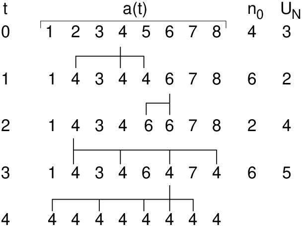
In Fig. 1 one sample evolution is shown. As visualized in the figure, at some random time, for a finite population size and if the total simulation time is large enough, all members population are for the first time offspring of the same individual which was present in the initial population (). Thus, they all have a common ancestor, i.e., for . We say the individual dominates the population. Thus, looking from this time backward to the initial configuration, which is statistically equivalent to looking forward, this time is the time to the most recent common ancestor we are interested in, i.e.,
Note that we measure the probability that any individual dominates (for the first time) after steps, which means we look forward in time. This probability is interestingly the same as the probability that a specific (say ) individual dominates after steps, conditioned that it is individual which dominates after some time, which basically means one starts at the time where one specific individual dominates, and looks backwards in time. This can be seen easily, because:
| (2) | |||||
| (3) | |||||
| (4) |
because by symmetry of all individuals and the conditional probabilities are all the same, thus the sum reduces to a multiplication with .
One can measure, for example, the mean of and obtain a (small-support) histogram via simple sampling: One generates, say, times a vector of random numbers, and runs each time the above described algorithm to generate the dynamics of the evolution. Then one measures for each run the resulting time where for the first time all members of the population originate from the same ancestor. Depending on the value of independent runs, the obtained histogram will be of better or worse quality. Typically, Probabilities of the order of can be measured, like .
II.2 Large-deviation approach
Following the description so far, one is able to simulate the evolution of the population in a standard way. The only difference to standard implementations is that the generation of the random numbers and the actual simulation of the stochastic target process are disentangled.
Nevertheless, this disentanglement allows one to perform a Markov-chain Monte Carlo evolution for the set : . Thus, the target process is not performed several times independently, but for a sequence of similar (correlated) sets (). This may appear inefficient on the first sight since the measured quantities , , , …will be correlated as well, in contrast to using each time a new set , corresponding to simple sampling. On the other hand, the MC evolution allows one to introduce a bias, such that the measured distribution for can be directed into a region of interest, e.g., where the original probabilities are very small. Here, since we are interested in the distribution of for a large range of the support, an exponential Boltzmann bias is used where is a freely adjustable parameter (a kind of artificial temperature), which allows us to center the observed distribution in different regions. Note that the choice corresponds to the absence of the bias, i.e., to the simple sampling presented in Sec. II.1, only including correlations. The bias is included in a standard Metropolis-Hastings algorithm where vectors () are sampled via changing a small fraction of entries of the current vector in each step. For details, please consider Ref. [27].
Note that this approach does not need any detailed knowledge about the specific model simulated, which is often used to “guide” a large-deviation approach to the region of interest. Thus, the approach is in contrast to many standard large-deviation algorithms for dynamical equilibrium and non-equilibrium systems [41]. Within the present approach the target process leading to the measurable quantity can be seen as a black box. This allows one to perform large-deviation measurements for almost arbitrary equilibrium and non-equilibrium processes which can be simulated on a computer using (pseudo) random numbers.

In Fig. 2 two sample evolutions of are shown as a function of the number of Monte Carlo steps. Both evolutions are for a population size , reproduction parameter and MC temperature . The negative temperature results in values of which are larger than typical values for this choice of and . Note that the two data sets start from opposite sides: one set is for a initial configuration vector which is drawn independently from . This corresponds to the typical behavior. The other vector is drawn such that it exhibits a preference for large values of . This is achieved by sampling the entries which are responsible for drawing the number of offspring not uniformly in the interval but in a smaller interval . In spite of the different initial conditions, after a while the value of the measured quantity agree within the range of the fluctuations. This indicates that the Markov chain has “forgotten” its initial condition, i.e., can be considered as equilibrated.
For each value of , one obtains a distribution which includes the original distribution under the bias . Such biased simulations have been performed already in the field of population biology, e.g., to estimate small likelihoods [31]. Nevertheless, here we are interested in obtaining the distribution of interest for a large range of the support, which has not been done in population genetics to our knowledge. To achieve this we have to perform the simulations for several values of and combine the results in a suitable way, as shortly outlined now. The sampled distribution at value is related to the original distribution [24] via
| (5) |
where is the normalization constant of , which can be determined from the numerical data, as explained next. By performing the simulation for suitably chosen values of , which have to be determined experimentally, one can cover a broad range of the desired distribution . If this is done such that the resulting distributions overlap for neighboring values of the temperature, say and , one can reconstruct the relative normalization constants from . Actually, several values of in the windows of overlap are considered and the mean-square difference in this window between the distributions obtained from (5) is minimized to obtain the “optimum” relative normalization constant . The last missing constraint is obtained from the overall normalization of which then results in the actual values for all normalization constants. Details can be found in Ref. [24], a generalization is explained in Ref. [42].
III Results
We have performed simulations for different population sizes , different values of the reproduction parameter and various temperatures . The number of different temperatures for a given combination of and ranged from two to seven.
For each combination of these parameters, the number of how many of the entries of the configuration vector were redrawn in each MC step to obtain the trial vector was adjusted. As a rule of thumb (often used for Monte Carlo simulation), this amount of adjustment was chosen such that the acceptance rate of the Metropolis steps was roughly near 0.5. Note that the number of changes for the entries of which are responsible for selecting the super parent, for selecting the number of offspring (), and for selecting the one-offspring parents (), were adjusted separately. The reason is that the amount of change for super parent entries and numbers of offspring entries have a higher influence on the acceptance rate than the amount of change for the one-offspring parent entries.

Using simple-sampling, we measured the mean of the time to the most recent common ancestor as a function of the population size . The result is shown in Fig. 3 using a logarithmically-scaled -axis. When ignoring very small values of , the data follows straight lines very well, meaning that it is described well by a logarithmic growth. This matches an analytical calculation for the uniform distribution, i.e., the case 11 1 The mean is stated in general in Ref. [44] after Eq. (37), see page 121. For the present case one has to perform a short calculation by using the corresponding measure which results in a dependence. very well. Also for -coalescent, a fast evolution is obtained [9]..

With increasing value of the typical number of descendants increases. Thus, one can expect that the mean decreases when increases. For the same reason one can expect that for the slope value decreases when increases. We have fitted the data to this functional form. The result is shown in Fig. 4 as a function of . Note that for we obtained which is compatible with . In the log-log plot, a straight line is visible for , meaning that converges to zero. Comparably, appears to converge to a finite value close to 1 (see inset of Fig. 4). This is reasonable because for the distribution of the number of descendants converges to the case where the super parent takes over the full population in one generation, independent of the size of the population, which means with and .
In the limit , diverges, i.e., the time grows more than logarithmically. This appears also to be reasonable, because in this limit the model converges to the Moran model, being equivalent to the Kingman coalescent, where for the time scale we use ( if the time is rescaled by as in the standard studies). Thus, in the general case , the evolutionary timescale grows much slower with increasing population size. This allows, as in the case of marine environments, for a much faster adaption to changing environments, if, e.g., selective pressure is present.

Next, we study the full distribution of , see Fig. 5 for the case , and different population sizes . This value corresponds to the uniform distribution and only for this case of a skewed offspring distribution for the extended Moran model rigorous results [17] are available to which we can compare. Using the large-deviation approach, we could measure the distribution over a large range of the support. Apparently these tails exhibit an exponential shape. We fitted these tails to functions for all values of . We obtained (), (), () (The error bars are just statistical error bars). All these values are very close to the exact value 22 2 See bottom of page 145 of Ref.[44]. and do within the fluctuations not depend on the population size. Thus, even small population sizes are suitable for obtaining results close to the limit, if the tails of the distribution are accessible. For this reason, we proceed with results for , for various values of .

We have performed extensive simulations for other values of , where no rigorous results are available. Since we were able to reproduce rigorous results for the test case , we are very confident that our results are reliable also for these other values of . In Fig. 6 the distributions for three different values of and a population size of are shown. Again, the tails of the distributions can be well fitted to exponential functions for all values of . We did this for all values of which we have studied.

In Fig. 7, the resulting behavior of as a function of is shown. With increasing value of , i.e., when the distribution of the number of offspring of the super parent is more and more located at large values, the value of decreases, corresponding to smaller times it takes for one individual to dominate the full distribution. Thus, for we obtain corresponding to an .
For the opposite limit the model converges to the classical Moran model [4], this corresponds to the Kingman coalescent for the -coalescent. Here, the exactly-known distribution of follows (see Eq. (53) and below in Ref. [43]) in the tails a simple exponential distribution . This corresponds to a value which evaluates for the present case () to , i.e. very close to 1, as shown in the figure. This means the distribution becomes, without rescaling the time, infinitely long stretched for the Moran model in the case . On the other hand, the extended Moran model for apparently all values of , even the smallest ones, shows a completely different behavior, all distributions fall off exponentially even in the limit . This corresponds to the slow logarithmic growth of the average .


Finally, we want to understand what leads during the evolution of a population to particular small or large value of . For this purpose, we study the correlation between the average value of the number of descendants encountered during an evolution and relate it to the value of . As shown in Fig. 8, very small values of correspond to untypical large values of the number of descendants, while slow evolutions, i.e., large values of correspond typically to small number of descendants. Note that the full range of correlations is only accessible to us because we used the large-deviation approach. The high-probability simple-sampling range is only within the first 10% of the range of values for . The observed behavior is somehow expected because many decedents lead clearly to a faster evolution of the population. The general result holds for all values of . One is tempted to assume that extreme long evolutions to the MRCA are created by periods with even smaller number of descendants. This could be caused in real environments, e.g., by long periods of low but not extremely low availability of nutrition. Interestingly, in the tail of the distribution, i.e., for very large values of , the values of drop only very slightly when increasing . This means, extreme long evolutions to the MRCA are rather an effect of rare choices of the particular sets of descendants, with a still considerable large number of descendants. Also, the shapes of the scatter plots look very similar for all values of the reproduction parameter . For the smaller value of the reproduction parameter, the variation of is smaller and farther away from the unconditional expectation value . This also appears to be reasonable, because the distribution falls off much quicker for small values of , thus cannot vary much during an evolution such as to result in a long evolution until the MRCA.
IV Summary and Discussion
We have studied the extended Moran model, where possibly a large fraction of the population is exchanged between two generations. This model is suitable, e.g., to describe in a simplified way the population dynamics in marine environments. We have studied a Beta()-distribution for the fraction of the population which descends from the super parent, as introduced in Ref. [38]. The variation of the parameter covers a large range of possible distributions, including the Moran case, the uniform distribution and the limit of a complete exchange of the full population. In particular we have studied the time to the most-recent common ancestor, which describes the timescale on which the genetic drift takes place. The typical behavior (like the mean) of this quantity can be readily studied.
Nevertheless, in order to describe the statistics of this model as comprehensively as possible, we investigated not only the typical behavior but also the distribution of for a range of the support as large as possible, including very small probabilities. Here, analytical results are only available for the cases of a uniform distribution, i.e., , and for the case which is the original Moran model. To access these distributions numerically for arbitrary values of , we used an established but elaborate statistical mechanics-based biased sampling approach. It is based on a Markov chain evolution of a vector of uniformly distributed random numbers from the interval , seen as an input vector to an arbitrary stochastic process.
We found that the mean time depends for all values logarithmically on the population size and converges to a constant for . This is in contrast to the quadratic behavior of the standard Moran model, and reflects a much faster evolution of a population, as observed for studies of the -coalescent and in previous experimental work on marine populations.
The distribution of shows an exponential behavior in the tails. For the cases and (where the “exponential” becomes infinitely strongly stretched for ) both mean as well as tail behavior are compatible with previous analytical results. By studying the correlations of to the history of the evolutions, we could show that medium rare deviations are caused by unlikely small numbers of descendants, while the strongest deviations are caused by a combination of small but not too small numbers of descendants and unlikely combinations of selected offspring.
This work also shows, in line with previous applications in other fields, that using sophisticated sampling techniques, the distributions of measurable quantities in population models can be studied over large ranges of the support. This allows one to access results in regions where no analytical results are available, as here for the extended Moran model. It would be interesting to apply such techniques to more refined models, such models with varying population size, or including selection, or models having a spatio-temporal evolution.
Acknowledgements.
We thank Charlotte Lotze and Hendrik Schawe for critically reading the manuscript. AKH is grateful to the Université Cergy-Pontoise for financing a two-month visit in 2016, during which the main parts of the project were performed. The simulations were performed on the HPC clusters HERO and CARL of the University of Oldenburg jointly funded by the DFG through its Major Research Instrumentation Programme (INST 184/108-1 FUGG and INST 184/157-1 FUGG) and the Ministry of Science and Culture (MWK) of the Lower Saxony State.References
- [1] M. Kot, Elements of Mathematical Ecology (Cambridge University Press, Cambridge, 2008).
- [2] S. Wright, Genetics 16, 97 (1931), ISSN 0016-6731.
- [3] W. J. Ewens, Mathematical Population Genetics (Springer, Berlin, 1979).
- [4] P. Moran, Proc. Cambridge Philos. Soc. 54, 60 (1958).
- [5] N. A. Rosenberg and M. Nordborg, Nature Reviews Genetics 3, 3380 (2002).
- [6] J. F. C. Kingman, Stochastic Processes and their Applications 13, 235 (1982), ISSN 0304-4149.
- [7] D. Hedgecock and A. I. Pudovkin, Bull. Marine Sci. 87, 971 (2011), ISSN 0007-4977.
- [8] D. Hedgecock, in Genetics and Evolution of Aquatic Organisms, edited by A. Beaumont (Chapman and Hall, London, 1994).
- [9] B. Eldon and J. Wakeley, Genetics 172, 2621 (2006), ISSN 0016-6731.
- [10] O. Sargsyan and J. Wakeley, Theoretical Population Biology 74, 104 (2008), ISSN 0040-5809.
- [11] S. Matuszewski, M. E. Hildebrandt, G. Achaz, and J. D. Jensen, Genetics 208, 323 (2018), ISSN 0016-6731.
- [12] K. K. Irwin, S. Laurent, S. Matuszewski, S. Vuilleumier, L. Ormond, H. Shim, and J. D. Bank, C. Jensen, Heredity 117, 393 (2016).
- [13] A. Tellier and C. Lemaire, Molecular Ecology 23, 2637 (2014).
- [14] J. Pitman, Ann. Probab. 27, 1870 (1999).
- [15] S. Sagitov, J. Appl. Prob. 36, 1116 (1999), ISSN 00219002.
- [16] H. E. Stanley, An Introduction to Phase Transitions and Critical Phenomena (Oxford University Press, Oxford, 1971).
- [17] T. Huillet and M. Möhle, Theor. Popul. Biol. 87, 5–14 (2013).
- [18] N. Glansdorff, Y. Xu, and B. Labedan, Biology Direct 3, 29 (2008), ISSN 1745-6150.
- [19] R. R. Hudson, in Oxford Surveys in Evolutionary Biology, edited by D. Futuyam and J. Antonovics (Oxford University Press, Oxford, 1991), vol. 7, pp. 1–44.
- [20] R. R. Hudson, K. Bailey, D. Skarecky, J. Kwiatowski, and F. J. Ayala, Genetics 136, 1329 (1994), ISSN 0016-6731.
- [21] F. den Hollander, Large Deviations (American Mathematical Society, Providence, 2000).
- [22] H. Touchette, Physics Reports 478, 1 (2009), ISSN 0370-1573.
- [23] A. Dembo and O. Zeitouni, Large Deviations Techniques and Applications (Springer, Berlin, 2010).
- [24] A. K. Hartmann, Phys. Rev. E 65, 056102 (2002).
- [25] A. K. Hartmann, Eur. Phys. J. B 84, 627 (2011).
- [26] A. K. Hartmann, S. N. Majumdar, and A. Rosso, Phys. Rev. E 88, 022119 (2013).
- [27] A. K. Hartmann, Phys. Rev. E 89, 052103 (2014).
- [28] J. M. Hammersley and K. W. Morton, Math. Proc. Cambr. Phil. Soc. 52, 449 (1956), ISSN 1469-8064.
- [29] J. A. Bucklew, Introduction to rare event simulation (Springer-Verlag, New York, 2004).
- [30] L. Excoffier and G. Heckel, Nature Rev. Gen. 7 (2006), eprint 745–758.
- [31] M. Stephens and P. Donnelly, J. Royal. Stat. Soc. B 62, 605 (2000), ISSN 13697412.
- [32] C. Cannings, Adv. Appl. Probab. 6, 260– (1974).
- [33] C. Cannings, Adv. Appl. Probab. 7, 264– (1975).
- [34] E. Bolthausen and A.-S. Sznitman, Communications in Mathematical Physics 197, 247 (1998), ISSN 1432-0916.
- [35] K. Binder and A. Young, Rev. Mod. Phys. 58, 801 (1986).
- [36] M. Mézard, G. Parisi, and M. Virasoro, Spin glass theory and beyond (World Scientific, Singapore, 1987).
- [37] A. P. Young, ed., Spin glasses and random fields (World Scientific, Singapore, 1998).
- [38] J. Schweinsberg, Stoch. Process. Appl. 106, 107 (2003), ISSN 0304-4149.
- [39] G. E. Crooks and D. Chandler, Phys. Rev. E 64, 026109 (2001).
- [40] M. Galassi, J. Davies, J. Theiler, B. Gough, G. Jungman, M. Booth, and F. Rossi, GNU Scientific Library Reference Manual (Network Theory Ltd., Bristol, UK, 2006).
- [41] J. T. Berryman and T. Schilling, J. Chem. Phys. 133, 244101 (2010).
- [42] M. R. Shirts and J. D. Chodera, The Journal of Chemical Physics 129, 124105 (2008).
- [43] T. Huillet, Math. Popul. Stud. 23, 164 (2016).
- [44] T. Huillet, Journal of Statistics: Advances in Theory and Applications 7, 85 (2012).