跳到论文正文
W Papers独立论文阅读器 arXiv:1710.07278 论文正文 计算阅读时间 · 0%
引用这篇论文根据当前论文元数据生成,正式投稿前建议核对。


License: arXiv.org perpetual non-exclusive license
arXiv:1710.07278v3 [math.ST] 07 Sep 2018

Early stopping for statistical inverse problems
via truncated SVD estimation

\fnmsMarkus \snmReiß
Abstract

We consider truncated SVD (or spectral cut-off, projection) estimators for a prototypical statistical inverse problem in dimension DD. Since calculating the singular value decomposition (SVD) only for the largest singular values is much less costly than the full SVD, our aim is to select a data-driven truncation level m^∈{1,…,D}\widehat{m}\in\{1,\ldots,D\} only based on the knowledge of the first m^\widehat{m} singular values and vectors.

We analyse in detail whether sequential early stopping rules of this type can preserve statistical optimality. Information-constrained lower bounds and matching upper bounds for a residual based stopping rule are provided, which give a clear picture in which situation optimal sequential adaptation is feasible. Finally, a hybrid two-step approach is proposed which allows for classical oracle inequalities while considerably reducing numerical complexity.

{frontmatter}
\runtitle

Early stopping for truncated SVD

{aug}
\affiliation

Universität Potsdam, Germany

\address

Institut für Mathematik
Universität Potsdam, Germany
gilles.blanchard@math.uni-potsdam.de

{aug}
\affiliation

Université Paris-Dauphine & PSL, France

\address

CEREMADE
Université Paris-Dauphine & PSL, France
hoffmann@ceremade.dauphine.fr

{aug}
\runauthor

G. Blanchard, M. Hoffmann and M. Reiß

\affiliation

Humboldt-Universität zu Berlin, Germany

\address

Institut für Mathematik
Humboldt-Universität zu Berlin, Germany
mreiss@mathematik.hu-berlin.de

{keyword}

[class=AMS] \kwd65J20, 62G07

{keyword}\kwd

Linear inverse problems; Truncated SVD; Spectral cut-off; Early stopping. Discrepancy principle; Adaptive estimation; Oracle inequalities

1 Introduction and overview of results

1.1 Model

A classical model for statistical inverse problems is the observation of

Y=A​μ+δ​W˙Y=A\mu+\delta\dot{W} (1.1)

where A:H1→H2A:H_{1}\to H_{2} is a linear, bounded operator between real Hilbert spaces H1,H2H_{1},H_{2}, μ∈H1\mu\in H_{1} is the signal of interest, δ>0\delta>0 is the noise level and W˙\dot{W} is a Gaussian white noise in H2H_{2}, see e.g. Bissantz et al. [1], Cavalier [5] and the references therein. In any concrete situation the problem is discretised, for instance by using a Galerkin scheme projecting on finite element or other approximation spaces. Therefore we can assume H1=ℝDH_{1}=\R^{D}, H2=ℝPH_{2}=\R^{P} with possibly very large DD and PP. Since the discretisation of μ\mu is at our choice, we assume D≤PD\leq P, and that A:ℝD→ℝPA:\R^{D}\to\R^{P} is one-to-one. We transform (1.1) by the singular value decomposition (SVD) of AA into the Gaussian vector observation model

Yi=λiμi+δεi,i=1,…,D,Y_{i}=\lambda_{i}\mu_{i}+\delta\varepsilon_{i},\;\;i=1,\ldots,D, (1.2)

where λ1≥λ2≥⋯≥λD>0\lambda_{1}\geq\lambda_{2}\geq\cdots\geq\lambda_{D}>0 are the nonzero singular values of AA, (μi)1≤i≤D(\mu_{i})_{1\leq i\leq D} the coefficients of μ\mu in the orthonormal basis of singular vectors and (εi)1≤i≤D(\varepsilon_{i})_{1\leq i\leq D} are independent standard Gaussian random variables. The results will easily extend to subgaussian errors as discussed below.

Working in the SVD representation (1.2), the objective is to recover the signal μ=(μi)1≤i≤D\mu=(\mu_{i})_{1\leq i\leq D} with best possible accuracy from the data (Yi)1≤i≤D(Y_{i})_{1\leq i\leq D}. A classical method is to use the truncated SVD estimators (also called projection or spectral cut-off estimators) μ^(m)\widehat{\mu}^{(m)}, 0≤m≤D0\leq m\leq D, given by

μ^i(m)=𝟏(i≤m)λi−1Yi,i=1,…,D,{\widehat{\mu}}^{(m)}_{i}={\bf 1}(i\leq m)\lambda_{i}^{-1}Y_{i},\qquad i=1,\ldots,D, (1.3)

which are ordered with decreasing bias and increasing variance (w.r.t. mm). Choosing a suitable truncation index m^=m^​(Y)\widehat{m}=\widehat{m}(Y) from the observed data is the genuine problem of adaptive model selection. Typical methods use (generalized) cross validation, see e.g. Wahba [19], unbiased risk estimation, see e.g. Cavalier et al. [6], penalized empirical risk minimisation, see e.g. Cavalier and Golubev [7], or Lepski’s balancing principle for inverse problems, see e.g. Mathé and Pereverzev [15]. They all share the drawback that the estimators μ^(m)\widehat{\mu}^{(m)} have first to be computed for all values of 0≤m≤D0\leq m\leq D, and then be compared to each other in some way.

In this work, we are motivated by constraints due to the possible obstructive computational complexity of calculating the full SVD in high dimensions. We stress that the initial discretisation of the observation is generally based on a fixed scheme which does not deliver a representation of the observation vector YY in an SVD basis; nor is the full SVD basis of the discretized operator AA a priori available in general, so that it has to be computed on the fly. Since the calculation of the largest singular value and its corresponding subspace is much less costly, efficient numerical algorithms rely on deflation or locking methods, which achieve the desired accuracy for the larger singular values first and then iteratively achieve the accuracy also for the next smaller singular values. As a basic example the popular power method can be considered, which usually finds after a few vector-matrix multiplications the top eigenvalue-eigenvector pair (with exponentially small error in the iteration number), so that by iterative application the largest mm singular values and vectors are computed with roughly 𝒪⁡(m​D2){\mathcal{O}}(mD^{2}) multiplications compared to 𝒪⁡(D3){\mathcal{O}}(D^{3}) multiplications for a full SVD in a worst case scenario. We refer to the monograph by Saad [17] for a comprehensive exposition of the numerical methods.

We investigate the possibility of an approach which is both statistically efficient and sequential along the SVD in the following sense: we aim at early stopping methods, in which the truncated SVD estimators μ^(m)\widehat{\mu}^{(m)} for m=0,1,…,m=0,1,\ldots, are computed iteratively, a stopping rule decides to stop at some step m^\widehat{m} and then μ^(m^)\widehat{\mu}^{(\widehat{m})} is used as the estimator.

More generally, we envision our setting as a simple and prototypical model to study the scope of statistical adaptivity using iterative methods, which are widely used in computational statistics and learning. A notable feature of these methods is that not only the numerical, but also the statistical complexity (e.g., measured by the variance) increases with the number of iterations, so that early stopping is essential from both points of view. It is common to use stopping rules based on monitoring the residuals because the user has access without substantial additional cost to the residual norm. Observe that the computation of the residual norm ∥Y−A​μ^(m)∥2=∥Y∥2−∑i=1mYi2\lVert Y-A\widehat{\mu}^{(m)}\rVert^{2}=\lVert Y\rVert^{2}-\sum_{i=1}^{m}Y_{i}^{2} does not require the full SVD, but only the knowledge of the mm first coefficient and of the full norm ∥Y∥2\lVert Y\rVert^{2}, which is readily available. The properties of such rules have been well studied for deterministic inverse problems (e.g. the discrepancy principle, see Engl et al. [10]). In a statistical setting, minimax optimal solutions along the iteration path have been identified in different settings, see e.g. Yao et al. [20] for gradient descent learning, Blanchard and Mathé [3] for conjugate gradients, Raskutti, Wainwright and Yu [16] for (reproducing) kernel learning and Bühlmann and Hothorn [4] for the application to L2L^{2}-boosting. All these methods stop at a fixed iteration step11 1 The stopping rule in [16] for a random design setting is data-dependent because the distribution of the design is unknown. The stopping iteration becomes fixed when the design distribution is known, the target function belonging to the unit ball of the kernel space., depending on the prior knowledge of the smoothness of the unknown solution.

By contrast, our goal is to analyse an a posteriori early stopping rule based on monitoring the residual, which corresponds to proposals by practitioners in the absence of prior smoothness information. An analysis of such a stopping rule for quite general spectral estimators like Landweber iteration is provided in the companion paper [2]. Although the general results can also be applied to the truncated SVD method, we exhibit a more transparent analysis for this prototypical method which gives more satisfactory results: we establish coherent lower bounds and we obtain adaptivity in strong norm via the oracle property, while for more general spectral estimators only rate results over Sobolev-type classes can be achieved. Moreover, a hybrid two-step procedure enjoys full adaptivity for the truncated SVD-method.

1.2 Non-asymptotic oracle approach

Our approach is a priori non-asymptotic and concentrates on oracle optimality analysis for individual signals. The oracle approach compares the error of μ^(m^)\widehat{\mu}^{(\widehat{m})} to the minimal error among (μ^(m))m(\widehat{\mu}^{(m)})_{m} for any signal μ\mu individually, which entails optimal adaptation in minimax settings, see e.g. Cavalier [5].

The risk (mean integrated squared error) for a fixed truncated SVD estimator μ^(m)\widehat{\mu}^{(m)} obeys a standard squared bias-variance decomposition

𝔼⁡[‖μ^(m)−μ‖2]=Bm2​(μ)+Vm,\E\big[\|\widehat{\mu}^{(m)}-\mu\|^{2}\big]=B_{m}^{2}(\mu)+V_{m}\,,

where ∥∙∥\lVert{\scriptstyle\bullet}\rVert denotes the Euclidean norm in ℝD\R^{D}, and

Bm2​(μ)\displaystyle B_{m}^{2}(\mu) :=𝔼⁡[‖𝔼⁡[μ^(m)]−μ‖2]=∑i=m+1Dμi2,\displaystyle:=\E\big[\|\E[\widehat{\mu}^{(m)}]-\mu\|^{2}\big]=\textstyle\sum_{i=m+1}^{D}\mu_{i}^{2}, (1.4)
Vm\displaystyle V_{m} :=𝔼⁡[‖μ^(m)−𝔼⁡[μ^(m)]‖2]=δ2​∑i=1mλi−2.\displaystyle:=\E\big[\|\widehat{\mu}^{(m)}-\E[\widehat{\mu}^{(m)}]\|^{2}\big]=\textstyle\delta^{2}\sum_{i=1}^{m}\lambda_{i}^{-2}. (1.5)

In distinction with the weak norm quantities defined below, we call Bm​(μ)B_{m}(\mu) strong bias of μ\mu and VmV_{m} strong variance.

If we have access to the residual squared norm

Rm2:=‖Y−A​μ^(m)‖2=∥Y∥2−∥A​μ^(m)∥2=∑i=1D(Yi−λi​μ^i(m))2=∑i=m+1DYi2,\textstyle R_{m}^{2}:=\|Y-A\widehat{\mu}^{(m)}\|^{2}=\lVert Y\rVert^{2}-\lVert A\widehat{\mu}^{(m)}\rVert^{2}=\sum_{i=1}^{D}(Y_{i}-\lambda_{i}\widehat{\mu}_{i}^{(m)})^{2}=\sum_{i=m+1}^{D}Y_{i}^{2}, (1.6)

then Rm2−(D−m)​δ2R_{m}^{2}-(D-m)\delta^{2} gives some bias information due to

𝔼⁡[Rm2−(D−m)​δ2]=Bm,λ2​(μ), with Bm,λ2​(μ):=∑i=m+1Dλi2​μi2.\textstyle\E[R_{m}^{2}-(D-m)\delta^{2}]=B_{m,\lambda}^{2}(\mu),\quad\text{ with }\quad B_{m,\lambda}^{2}(\mu):=\sum_{i=m+1}^{D}\lambda_{i}^{2}\mu_{i}^{2}.

We call Bm,λ2​(μ)B_{m,\lambda}^{2}(\mu) the weak bias and similarly Vm,λ=m​δ2V_{m,\lambda}=m\delta^{2} the weak variance. They correspond to measuring the error in the weak norm (or prediction norm) ∥v∥λ2:=∥A​v∥2=∑i=1Dλi2​vi2\lVert v\rVert_{\lambda}^{2}:=\lVert Av\rVert^{2}=\sum_{i=1}^{D}\lambda_{i}^{2}v_{i}^{2}, which usually (always if λ1<1\lambda_{1}<1) is smaller than the strong Euclidean norm ∥∙∥\lVert{\scriptstyle\bullet}\rVert. The squared bias-variance decomposition for the weak risk then reads 𝔼⁡[‖μ^(m)−μ‖λ2]=Bm,λ2​(μ)+Vm,λ\E\big[\|\widehat{\mu}^{(m)}-\mu\|^{2}_{\lambda}\big]=B_{m,\lambda}^{2}(\mu)+V_{m,\lambda}. Our setting is thus a particular instance of the question raised by Lepski [13] whether adaptation in one loss (here: weak norm) leads to adaptation in another loss (here: strong norm). Our positive answer for truncated SVD or spectral cut-off estimation will also extend the results by Chernousova et al. [8].

Intrinsic to the sequential analysis is the fact that at truncation index mm we cannot say anything about the way the bias decreases for larger indices: it may drop to zero at m+1m+1 or even stay constant until D−1D-1. Even if we knew the exact value of the bias until index mm, we could not minimise the sum of squared bias and variance sequentially. Instead, we should wait until the squared bias is sufficiently small to equal (approximately) the variance. This leads to the notion of the strongly balanced oracle

m𝔰=m𝔰​(μ)\displaystyle m_{\mathfrak{s}}=m_{\mathfrak{s}}(\mu) :=min⁡{m∈{0,…,D}|Vm≥Bm2​(μ)},\displaystyle:=\min\{m\in\{0,\ldots,D\}\,|\,V_{m}\geq B_{m}^{2}(\mu)\}, (1.7)

whose risk is always upper bounded by twice the classical oracle risk, see (3.5) below.

1.3 Setting for asymptotic considerations

Risk estimates over classes of signals and asymptotics for vanishing noise level δ→0\delta\to 0 often help to reveal main features. This way, we can also provide lower bounds for sequential estimation procedures and compare them directly to classical minimax convergence rates. In our setting, the magnitude of the discretisation dimension DD plays a central role, so that it is sensible to assume in an asymptotic view that D=Dδ→∞D=D_{\delta}\rightarrow\infty as δ→0\delta\rightarrow 0. As classes of signals, we will consider the Sobolev-type ellipsoids

Hβ​(R,D):={μ∈ℝD|∑i=1Di2​β​μi2≤R2},β≥0,R>0,\textstyle H^{\beta}(R,D):=\{\mu\in\R^{D}\,|\,\sum_{i=1}^{D}i^{2\beta}\mu_{i}^{2}\leq R^{2}\},\;\;\beta\geq 0,R>0, (1.8)

and we shall use the following polynomial spectral decay assumption

CA−1​i−p≤λi≤CA​i−p,1≤i≤D,C_{A}^{-1}i^{-p}\leq\lambda_{i}\leq C_{A}i^{-p},\qquad 1\leq i\leq D, (PSD(p,CAp,C_{A}))

for p≥0p\geq 0, CA≥1C_{A}\geq 1. The spectrum is allowed to change with DD and δ\delta, but p,CAp,C_{A} are considered as fixed constants. Under these assumptions, standard computations yield for μ∈Hβ​(R,D)\mu\in H^{\beta}(R,D), 1≤m≤D1\leq m\leq D:

Bm2​(μ)≤R2​m−2​β;Vm≤CA−2​δ2​m2​p+1.B^{2}_{m}(\mu)\leq R^{2}m^{-2\beta}\,;\qquad V_{m}\leq C_{A}^{-2}\delta^{2}m^{2p+1}\,.

Balance between these squared bias and variance bounds is obtained for mm of the order of the minimax truncation “time”

tβ,p,R(δ):=(R−1δ)−2/(2β+2p+1),t_{\beta,p,R}(\delta):=(R^{-1}\delta)^{-2/(2\beta+2p+1)}, (1.9)

provided the condition D≥tβ,p,R​(δ)D\geq t_{\beta,p,R}(\delta) holds. This gives rise to the risk rate

ℛβ,p,R∗​(δ):=R​(R−1​δ)2​β/(2​β+2​p+1),{\cal R}^{*}_{\beta,p,R}(\delta):=R(R^{-1}\delta)^{2\beta/(2\beta+2p+1)},

which agrees with the optimal minimax rate in the standard Gaussian sequence model (i.e. D=∞D=\infty). On the other hand, for D≲tβ,p,R​(δ)D\lesssim t_{\beta,p,R}(\delta) the choice m=Dm=D is optimal on Hβ​(R,D)H^{\beta}(R,D) and the rate degenerates to 𝒪⁡(D2​p+1​δ2)\mathcal{O}(D^{2p+1}\delta^{2}). This situation is indicative of an insufficient discretisation and will be excluded from the asymptotic considerations.

1.4 Overview of results

Our results consist of lower and upper bounds for sequentially adaptive stopping rules. The stopping rules permitted are most conveniently described in terms of stopping times with respect to an appropriate filtration. Introduce the frequency filtration

ℱm:=σ⁡(μ^(0),…,μ^(m))=σ⁡(Y1,…,Ym),\mathcal{F}_{m}:=\sigma\big(\widehat{\mu}^{(0)},\ldots,\widehat{\mu}^{(m)}\big)=\sigma\big(Y_{1},\ldots,Y_{m}\big), (1.10)

ℱ0\mathcal{F}_{0} being the trivial sigma-field. Stopping rules with respect to the filtration ℱ=(ℱm)0≤m≤D\mathcal{F}=(\mathcal{F}_{m})_{0\leq m\leq D} must decide whether to halt and output μ^(m)\widehat{\mu}^{(m)} based only on the information of the first mm estimators. Statistical adaptation will turn out to be essentially impossible for such stopping rules (Section 2.1). If the residual (1.6) is available at no substantial computational cost, taking this information into account, we define the residual filtration

𝒢m:=ℱm∨σ⁡(R02,…,Rm2)=ℱm∨σ⁡(‖Y‖2),\mathcal{G}_{m}:=\mathcal{F}_{m}\vee\sigma(R_{0}^{2},\ldots,R_{m}^{2})=\mathcal{F}_{m}\vee\sigma\big(\|Y\|^{2}\big), (1.11)

which is the filtration ℱm\mathcal{F}_{m} enlarged by the residuals up to index mm.

Pushing some technical details aside, the main message conveyed by our lower bounds is that oracle statistical adaptation with respect to the residual filtration is impossible for signals μ\mu such that the strongly balanced oracle m𝔰​(μ)m_{\mathfrak{s}}(\mu) is o⁡(D)o(\sqrt{D}). (Section 2.2). On the other hand, we establish in Section 3 that this statement is sharp, in the sense that the simple residual-based stopping rule

τ=min⁡{m≥m0|Rm2≤κ},\tau=\min\big\{m\geq m_{0}\,|\,R_{m}^{2}\leq\kappa\big\}, (1.12)

with a proper choice of κ\kappa and m0m_{0} is statistically adaptive for signals μ\mu such that m𝔰​(μ)≳Dm_{\mathfrak{s}}(\mu)\gtrsim\sqrt{D}. Let us stress that by minimax adaptive we always mean that the procedure attains the optimal rate even among all methods with access to the entire data, that is without information constraints.

Finally, in Section 4 we introduce a hybrid two-step approach consisting of the above stopping rule with m0∼D​log⁡Dm_{0}\sim\sqrt{D}\log D, followed by a traditional (non-sequential) model selection procedure over m≤m0m\leq m_{0}, in the case where τ=m0\tau=m_{0} (immediate stop hinting at an optimal index smaller than m0m_{0}). This procedure enjoys full oracle adaptivity at a computational cost of calculating on average the first 𝒪⁡(max⁡(D​log⁡D,m𝔰​(μ))){\mathcal{O}}(\max(\sqrt{D}\log D,m_{\mathfrak{s}}(\mu))) singular values, to be compared to the full SVD with DD singular values in non-sequential adaptation. Some numerical simulations illustrate the theoretical analysis. Technical proofs are gathered in an appendix.

2 Lower bounds

2.1 The frequency filtration

Let τ\tau be an ℱ\mathcal{F}-stopping time, where ℱ\mathcal{F} is the frequency filtration defined in (1.10) and let22 2 We emphasise in the notation the dependence on μ\mu in the distribution of τ\tau and the YiY_{i} by adding the subscript μ\mu when writing the expectation 𝔼=𝔼μ\E=\E_{\mu} or probability P=PμP=P_{\mu}.

ℛ​(μ,τ)2:=𝔼μ⁡[∥μ^(τ)−μ∥2].{\cal R}(\mu,\tau)^{2}:=\E_{\mu}[\lVert\widehat{\mu}^{(\tau)}-\mu\rVert^{2}].

By Wald’s identity, we obtain the simple formula

ℛ​(μ,τ)2=𝔼μ⁡[∑i=τ+1Dμi2+∑i=1τλi−2​δ2​εi2]=𝔼μ⁡[Bτ2​(μ)+Vτ],\textstyle{\cal R}(\mu,\tau)^{2}=\E_{\mu}\big[\sum_{i=\tau+1}^{D}\mu_{i}^{2}+\sum_{i=1}^{\tau}\lambda_{i}^{-2}\delta^{2}\varepsilon_{i}^{2}\big]=\E_{\mu}\big[B_{\tau}^{2}(\mu)+V_{\tau}\big], (2.1)

with Bm2​(μ)B_{m}^{2}(\mu) and VmV_{m} from (1.4), (1.5). This implies in particular that an oracle stopping time, i.e., an optimal ℱ\mathcal{F}-stopping time constructed using the knowledge of μ\mu, coincides with the deterministic oracle argminm⁡(Bm2​(μ)+Vm)\argmin_{m}\big(B_{m}^{2}(\mu)+V_{m}\big) almost surely. The next proposition encapsulates the main argument for the lower bound and merely relies on a two-point analysis. It clarifies that if the stopping time τ\tau yields a squared risk comparable to the optimally balanced risk for a given signal μ\mu, then this signal can be changed arbitrarily to μ¯\bar{\mu} after the index ⌊3​C​m𝔰​(μ)⌋\lfloor 3Cm_{\mathfrak{s}}(\mu)\rfloor, while the risk for the rule τ\tau always stays larger than the squared bias of that part – which can be made arbitrarily large by “hiding” signal in large-index coefficients.

2.1 Proposition.

Let μ,μ¯∈ℝD\mu,\bar{\mu}\in\R^{D} with μi=μ¯i\mu_{i}=\bar{\mu}_{i} for all i≤i0i\leq i_{0} and i0∈{1,…,D−1}i_{0}\in\{1,\ldots,D-1\}. Then any ℱ\mathcal{F}-stopping rule τ\tau satisfies

ℛ​(μ¯,τ)2≥Bi02​(μ¯)​(1−ℛ​(μ,τ)2Vi0+1).{\cal R}(\bar{\mu},\tau)^{2}\geq B_{i_{0}}^{2}(\bar{\mu})\Big(1-\frac{{\cal R}(\mu,\tau)^{2}}{V_{i_{0}+1}}\Big).

Suppose ℛ​(μ,τ)2≤C​ℛ​(μ,m𝔰)2{\cal R}(\mu,\tau)^{2}\leq C{\cal R}(\mu,m_{\mathfrak{s}})^{2} for the balanced oracle m𝔰m_{\mathfrak{s}} in (1.7) and some C≥1C\geq 1. Then for any μ¯∈ℝD\bar{\mu}\in\R^{D} with μ¯i=μi\bar{\mu}_{i}=\mu_{i} for i≤3​C​m𝔰i\leq 3Cm_{\mathfrak{s}} we obtain

ℛ​(μ¯,τ)2≥13​B⌊3​C​m𝔰⌋2​(μ¯).{\cal R}(\bar{\mu},\tau)^{2}\geq\tfrac{1}{3}B_{\lfloor 3Cm_{\mathfrak{s}}\rfloor}^{2}(\bar{\mu}).
Proof.

We use the fact that (Yi)1≤i≤i0(Y_{i})_{1\leq i\leq i_{0}} has the same law under PμP_{\mu} and Pμ¯P_{\bar{\mu}} and so has 𝟏​(τ≤i0){\bf 1}(\tau\leq i_{0}) by the stopping time property of τ\tau. Moreover, thanks to the monotonicity of m↦Vmm\mapsto V_{m} and m↦Bm2​(μ¯)m\mapsto B_{m}^{2}(\bar{\mu}), Markov’s inequality and identity (2.1):

ℛ​(μ¯,τ)2\displaystyle{\cal R}(\bar{\mu},\tau)^{2} ≥𝔼μ¯⁡[Bτ2​(μ¯)​𝟏​(τ≤i0)]\displaystyle\geq\E_{\bar{\mu}}[B_{\tau}^{2}(\bar{\mu}){\bf 1}(\tau\leq i_{0})]
=𝔼μ⁡[Bτ2​(μ¯)​𝟏​(τ≤i0)]\displaystyle=\E_{\mu}[B_{\tau}^{2}(\bar{\mu}){\bf 1}(\tau\leq i_{0})]
≥Bi02​(μ¯)​Pμ​(τ≤i0)\displaystyle\geq B_{i_{0}}^{2}(\bar{\mu})P_{\mu}(\tau\leq i_{0})
≥Bi02​(μ¯)​(1−Pμ​(Vτ≥Vi0+1))\displaystyle\geq B_{i_{0}}^{2}(\bar{\mu})(1-P_{\mu}(V_{\tau}\geq V_{i_{0}+1}))
≥Bi02​(μ¯)​(1−𝔼μ⁡[Vτ]Vi0+1)\displaystyle\geq B_{i_{0}}^{2}(\bar{\mu})\Big(1-\frac{\E_{\mu}[V_{\tau}]}{V_{i_{0}+1}}\Big)
≥Bi02​(μ¯)​(1−ℛ​(μ,τ)2Vi0+1).\displaystyle\geq B_{i_{0}}^{2}(\bar{\mu})\Big(1-\frac{{\cal R}(\mu,\tau)^{2}}{V_{i_{0}+1}}\Big).

The second assertion follows by inserting i0=⌊3​C​m𝔰⌋i_{0}=\lfloor 3Cm_{\mathfrak{s}}\rfloor and ℛ​(μ,τ)2≤2​C​Vm𝔰{\cal R}(\mu,\tau)^{2}\leq 2CV_{m_{\mathfrak{s}}} together with Vm𝔰/Vi0+1≤m𝔰/(i0+1)V_{m_{\mathfrak{s}}}/V_{i_{0}+1}\leq m_{\mathfrak{s}}/(i_{0}+1) since the singular values λi\lambda_{i} are non-increasing. ∎

In Appendix 5.1 we use this proposition to provide a result suitable for asymptotic interpretation (we use the notation from Section 1.3):

2.2 Corollary.

Assume (PSD( p , C A )) and let τ\tau be any ℱ\mathcal{F}-stopping rule. If there exists μ∈Hβ​(R,D)\mu\in H^{\beta}(R,D) with ℛ⁡(μ,τ)≤Cμ​ℛβ,p,R∗​(δ){\cal R}(\mu,\tau)\leq C_{\mu}{\cal R}^{*}_{\beta,p,R}(\delta), then for any α∈[0,β]\alpha\in[0,\beta], R¯≥2​R\bar{R}\geq 2R, there exists μ¯∈Hα​(R¯,D)\bar{\mu}\in H^{\alpha}(\bar{R},D) such that

ℛ⁡(μ¯,τ)≥c1​R¯​(R−1​δ)2​α/(2​β+2​p+1),{\cal R}(\bar{\mu},\tau)\geq c_{1}\bar{R}(R^{-1}\delta)^{2\alpha/(2\beta+2p+1)}\,,

provided D≥c2​tβ,p,R​(δ)D\geq c_{2}t_{\beta,p,R}(\delta). The constants c1,c2>0c_{1},c_{2}>0 only depend on CμC_{\mu} and CAC_{A}.

The conclusion for impossible rate-optimal adaptation is a direct consequence of Corollary 2.2: since for any α<β\alpha<\beta the rate δ2​α/(2​β+2​p+1)\delta^{2\alpha/(2\beta+2p+1)} is suboptimal, no ℱ{\cal F}-stopping rule can adapt over Sobolev classes with different regularities. Finally, the rate R¯​(R−1​δ)2​α/(2​β+2​p+1)\bar{R}(R^{-1}\delta)^{2\alpha/(2\beta+2p+1)} is attained by a deterministic stopping rule that stops at the oracle frequency for Hβ​(R,D)H^{\beta}(R,D), so that the lower bound is in fact a sharp no adaptation result.

2.2 Residual filtration

We start with a key lemma, similar in spirit to the first step in the proof of Proposition 2.1, but valid for an arbitrary random τ\tau. Here and in the sequel the numerical values are not optimised, but give rise to more transparent proofs and convey some intuition for the worst case order of magnitude. The proof is delayed until Appendix 5.2.

2.3 Lemma.

Let τ=τ⁡((Yi)1≤i≤D)∈{0,…,D}\tau=\tau\big((Y_{i})_{1\leq i\leq D}\big)\in\{0,\ldots,D\} be an arbitrary (measurable) data-dependent index. Then for any m∈{1,…,D}m\in\{1,\ldots,D\} the following implication holds true:

Vm≥200​ℛ​(μ,τ)2⇒Pμ​(τ≥m)≤0.9.V_{m}\geq 200\,{\mathcal{R}}(\mu,\tau)^{2}\Rightarrow P_{\mu}(\tau\geq m)\leq 0.9.

For 𝒢\mathcal{G}-stopping rules, where 𝒢\mathcal{G} is the residual filtration defined in (1.11), we deduce the following lower bound, again based on a two-point argument:

2.4 Proposition.

Let τ\tau be an arbitrary 𝒢{\cal G}-stopping rule. Consider μ∈ℝD\mu\in\R^{D} and i0∈{1,…,D}i_{0}\in\{1,\ldots,D\} such that Vi0+1≥ 200​ℛ​(μ,τ)2V_{i_{0}+1}\geq\,200{\cal R}(\mu,\tau)^{2}. Then

ℛ​(μ¯,τ)2≥0.05​Bi02​(μ¯){\cal R}(\bar{\mu},\tau)^{2}\geq 0.05B_{i_{0}}^{2}(\bar{\mu})

holds for any μ¯∈ℝD\bar{\mu}\in\R^{D} that satisfies

  1. (a)

    μi=μ¯i\mu_{i}=\bar{\mu}_{i} for all i≤i0i\leq i_{0},

  2. (b)

    the weak bias bound |Bi0,λ2​(μ¯)−Bi0,λ2​(μ)|≤0.05​D−i02​δ2\lvert B_{i_{0},\lambda}^{2}(\bar{\mu})-B_{i_{0},\lambda}^{2}(\mu)\rvert\leq 0.05\frac{\sqrt{D-i_{0}}}{2}\delta^{2} and

  3. (c)

    Bi0,λ​(μ)+Bi0,λ​(μ¯)≥5.25​δB_{i_{0},\lambda}(\mu)+B_{i_{0},\lambda}(\bar{\mu})\geq 5.25\delta.

Suppose that ℛ​(μ,τ)2≤Cμ​ℛ​(μ,m𝔰)2{\cal R}(\mu,\tau)^{2}\leq C_{\mu}{\cal R}(\mu,m_{\mathfrak{s}})^{2} holds with some Cμ≥1C_{\mu}\geq 1. Then any i0≥400​Cμ​m𝔰i_{0}\geq 400C_{\mu}m_{\mathfrak{s}} will satisfy the initial requirement.

Proof.

First, we lower bound the risk of μ¯\bar{\mu} by its bias on {τ≤i0}\{\tau\leq i_{0}\} and then transfer to the law of τ\tau under PμP_{\mu}, using the total variation distance on 𝒢i0{\cal G}_{i_{0}}:

ℛ​(μ¯,τ)2\displaystyle{\cal R}(\bar{\mu},\tau)^{2} ≥𝔼μ¯⁡[Bτ2​(μ¯)​𝟏​(τ≤i0)]\displaystyle\geq\E_{\bar{\mu}}[B_{\tau}^{2}(\bar{\mu}){\bf 1}(\tau\leq i_{0})]
≥Bi02​(μ¯)​Pμ¯​(τ≤i0)\displaystyle\geq B_{i_{0}}^{2}(\bar{\mu})P_{\bar{\mu}}(\tau\leq i_{0})
≥Bi02​(μ¯)​(Pμ​(τ≤i0)−∥Pμ−Pμ¯∥T​V​(𝒢i0)).\displaystyle\geq B_{i_{0}}^{2}(\bar{\mu})\big(P_{\mu}(\tau\leq i_{0})-\lVert P_{\mu}-P_{\bar{\mu}}\rVert_{TV({\cal G}_{i_{0}})}\big).

By Lemma 2.3 we infer Pμ​(τ≤i0)≥0.1P_{\mu}(\tau\leq i_{0})\geq 0.1. Denote Wi0=(Y1,…,Yi0)W_{i_{0}}=(Y_{1},\ldots,Y_{i_{0}}). Since the law of Wi0W_{i_{0}} is identical under PμP_{\mu} and Pμ¯P_{\bar{\mu}}, and Wi0W_{i_{0}} is independent of Ri02R^{2}_{i_{0}} for both measures, the total variation distance between PμP_{\mu} and Pμ¯P_{\bar{\mu}} on 𝒢i0{\cal G}_{i_{0}} equals the total variation distance between the respective laws of the scaled residual δ−2​Ri02\delta^{-2}R_{i_{0}}^{2}. For ϑ∈ℝD\vartheta\in\R^{D}, let ℙKϑ\PP_{K}^{\vartheta} be the non-central χ2\chi^{2}-law of Xϑ=∑k=1K(ϑk+Zk)2X_{\vartheta}=\sum_{k=1}^{K}(\vartheta_{k}+Z_{k})^{2} with ZkZ_{k} independent and standard Gaussian. With K=D−i0K=D-i_{0}, ϑk=δ−1​λi0+k​μi0+k\vartheta_{k}=\delta^{-1}\lambda_{i_{0}+k}\mu_{i_{0}+k}, ϑ¯k=δ−1​λi0+k​μ¯i0+k\bar{\vartheta}_{k}=\delta^{-1}\lambda_{i_{0}+k}\bar{\mu}_{i_{0}+k}, the total variation distance between the respective laws of the scaled residual δ−2​Ri02\delta^{-2}R_{i_{0}}^{2} exactly equals ‖ℙKϑ−ℙKϑ¯‖TV\|\PP_{K}^{\vartheta}-\PP_{K}^{\bar{\vartheta}}\|_{TV}. By Lemma 5.1 in the Appendix, taking account of ∥ϑ∥=δ−1​Bi0,λ​(μ)\lVert\vartheta\rVert=\delta^{-1}B_{i_{0},\lambda}(\mu) and similarly for ∥ϑ¯∥\lVert\bar{\vartheta}\rVert, we infer from (c) the simplified bound

∥Pμ−Pμ¯∥T​V​(𝒢i0)≤2​|Bi0,λ2​(μ¯)−Bi0,λ2​(μ)|δ2​D−i0.\lVert P_{\mu}-P_{\bar{\mu}}\rVert_{TV({\cal G}_{i_{0}})}\leq\frac{2\lvert B_{i_{0},\lambda}^{2}(\bar{\mu})-B_{i_{0},\lambda}^{2}(\mu)\rvert}{\delta^{2}\sqrt{D-i_{0}}}.

Under our assumption on μ¯\bar{\mu}, this is at most 0.05, and the inequality follows. From ℛ​(μ,τ)2≤2​Cμ​Vm𝔰{\cal R}(\mu,\tau)^{2}\leq 2C_{\mu}V_{m_{\mathfrak{s}}} and Vi0+1/Vm𝔰≥(i0+1)/m𝔰V_{i_{0}+1}/V_{m_{\mathfrak{s}}}\geq(i_{0}+1)/m_{\mathfrak{s}}, the last statement follows. ∎

In comparison with the frequency filtration, the main new hypothesis is that at i0i_{0} the weak bias of μ¯\bar{\mu} is sufficiently close to that of μ\mu, while the lower bound is still expressed in terms of the strong bias. This is natural since the bias only appears in weak form in the residuals, while the risk involves the strong bias. Condition (c) is just assumed to simplify the bound. To obtain valuable counterexamples, μ¯\bar{\mu} is usually chosen at maximal weak bias distance of μ\mu allowed by (b), so that (c) is always satisfied in the interesting cases where D−i0\sqrt{D-i_{0}} is not small.

Considering the behaviour over Sobolev-type ellipsoids, we obtain in Appendix 5.4 a lower bound result comparable to Corollary 2.2 for the frequency filtration.

2.5 Corollary.

Assume (PSD( p , C A )) and let τ\tau be any 𝒢\mathcal{G}-stopping time. If there exists μ∈Hβ​(R,D)\mu\in H^{\beta}(R,D) with ℛ⁡(μ,τ)≤Cμ​ℛβ,p,R∗​(δ){\cal R}(\mu,\tau)\leq C_{\mu}{\cal R}^{*}_{\beta,p,R}(\delta), then for any α∈[0,β]\alpha\in[0,\beta]  and R¯≥2​R\bar{R}\geq 2R, there exists μ¯∈Hα​(R¯,D)\bar{\mu}\in H^{\alpha}(\bar{R},D) such that

ℛ⁡(μ¯,τ)≥c1​R¯​min⁡((R¯−1​δ​D1/4)2​α/(2​α+2​p),(R−1​δ)2​α/(2​β+2​p+1)),{\cal R}(\bar{\mu},\tau)\geq c_{1}\bar{R}\min\Big(\big(\bar{R}^{-1}\delta D^{1/4}\big)^{2\alpha/(2\alpha+2p)},\,(R^{-1}\delta)^{2\alpha/(2\beta+2p+1)}\Big),

provided R−1​δ≤c2R^{-1}\delta\leq c_{2} and D≥c3​tα−14,p,R¯​(δ)D\geq c_{3}t_{\alpha-\frac{1}{4},p,\bar{R}}(\delta) . The constants c1,c3>0c_{1},c_{3}>0, and c2∈(0,1]c_{2}\in(0,1] depend only on Cμ,CA,α,pC_{\mu},C_{A},\alpha,p.

The form of the lower bound is transparent: as in the case of the frequency filtration, the sub-obtimal rate R¯​(R−1​δ)2​α/(2​β+2​p+1)\bar{R}(R^{-1}\delta)^{2\alpha/(2\beta+2p+1)} is the one attained by a deterministic rule that stops at the oracle frequency for Hβ​(R,D)H^{\beta}(R,D), whereas R¯​(R¯−1​δ​D1/4)2​α/(2​α+2​p)\bar{R}\big(\bar{R}^{-1}\delta D^{1/4}\big)^{2\alpha/(2\alpha+2p)} is the size of a signal that may be hidden in the noise of the residual, i.e., is not detected with positive probability by any test, thus also leading to erroneous early stopping. Note that for the direct problem (p=0p=0), the latter quantity is just δ​D1/4\delta D^{1/4}, which is exactly the critical signal strength in nonparametric testing, see Ingster and Suslina [11], while for p>0p>0, it reflects the interplay between the weak bias part in the residual and the strong bias part in the risk within the Sobolev ellipsoid.

Corollary 2.5 implies in turn explicit constraints for the maximal Sobolev regularity to which a 𝒢\mathcal{G}-stopping rule can possibly adapt. Here, we argue asymptotically and let explicitly D=DδD=D_{\delta} tend to infinity as the noise level δ\delta tends to zero. In this setting, a stopping rule τ\tau is to be understood as a family of stopping rules that depend on the knowledge of DD and δ\delta.

2.6 Corollary.

Assume (PSD( p , C A )). Let β+>β−≥0\beta_{+}>\beta_{-}\geq 0, R+,R−>0R_{+},R_{-}>0. Suppose that there exists a 𝒢{\cal G}-stopping rule τ\tau such that ℛ⁡(μ,τ)≤C​ℛβ,p,R∗​(δ){\cal R}(\mu,\tau)\leq C\mathcal{R}^{*}_{\beta,p,R}(\delta) holds for some C>0C>0, all δ>0\delta>0 small enough, and for every μ∈Hβ​(R,Dδ)\mu\in H^{\beta}(R,D_{\delta}), simultaneously for (β,R)∈{(β−,R−),(β+,R+)}(\beta,R)\in\{(\beta_{-},R_{-}),(\beta_{+},R_{+})\}. Then the rate-optimal truncation time for Hβ−​(R−,Dδ)H^{\beta_{-}}(R_{-},D_{\delta}) must satisfy Dδ=𝒪​(tβ−,p,R−​(δ))\sqrt{D_{\delta}}={\mathcal{O}}(t_{\beta_{-},p,R_{-}}(\delta)) as δ→0\delta\to 0 (all other parameters being fixed).

In particular, if a 𝒢{\cal G}-stopping rule τ\tau is rate-optimal over Hβ​(R,Dδ)H^{\beta}(R,D_{\delta}) for β∈[βm​i​n,βm​a​x]\beta\in[\beta_{min},\beta_{max}], βm​a​x>βm​i​n≥0\beta_{max}>\beta_{min}\geq 0, and some R>0R>0, then we necessarily must have βm​a​x≤lim infδ→0log⁡δ−2log⁡Dδ−p−1/2\beta_{max}\leq\liminf_{\delta\to 0}\frac{\log\delta^{-2}}{\log D_{\delta}}-p-1/2.

Proof.

In this proof we denote by ’≲\lesssim’, ’≳\gtrsim’ inequalities holding up to factors depending on CA,p,β+,β−,R−,R+C_{A},p,\beta_{+},\beta_{-},R_{-},R_{+}. We apply Corollary 2.5 with β=β+\beta=\beta_{+}, α=β−\alpha=\beta_{-} and R¯=R−\bar{R}=R_{-}, R=min⁡(R+,R¯/2)R=\min(R_{+},\bar{R}/2). Because of δ−2/(2β−+2p+1/2)≤δ−4/(2β−+2p+1)=o(Dδ)\delta^{-2/(2\beta_{-}+2p+1/2)}\leq\delta^{-4/(2\beta_{-}+2p+1)}=o(D_{\delta}), the conditions are fulfilled for sufficiently small δ>0\delta>0 and we conclude (R+,R−R_{+},R_{-} are fixed)

∃μ¯∈Hβ−​(R−,D):ℛ⁡(μ¯,τ)≳min⁡((δ​Dδ1/4)2​β−/(2​β−+2​p),δ2​β−/(2​β++2​p+1)).\exists\bar{\mu}\in H^{\beta_{-}}(R_{-},D):\;{\cal R}(\bar{\mu},\tau)\gtrsim\min\Big(\big(\delta D_{\delta}^{1/4}\big)^{2\beta_{-}/(2\beta_{-}+2p)},\,\delta^{2\beta_{-}/(2\beta_{+}+2p+1)}\Big).

By assumption, that rate must be 𝒪⁡(δ2​β−/(2​β−+2​p+1)){\mathcal{O}}(\delta^{2\beta_{-}/(2\beta_{-}+2p+1)}). Since the second term in the above minimum is of larger order than this, this must imply (δ​Dδ1/4)2​β−/(2​β−+2​p)≲δ2​β−/(2​β−+2​p+1)(\delta D_{\delta}^{1/4})^{2\beta_{-}/(2\beta_{-}+2p)}\lesssim\delta^{2\beta_{-}/(2\beta_{-}+2p+1)}, and further Dδ≲δ−2/(2β−+2p+1)≲tβ−,p,R−(δ).\sqrt{D_{\delta}}\lesssim\delta^{-2/(2\beta_{-}+2p+1)}\lesssim t_{\beta_{-},p,R_{-}}(\delta). The first statement is proved.

For the second assertion, we proceed by contradiction and assume βm​a​x>βl​i​m:=lim infδ→0log⁡δ−2log⁡Dδ−p−1/2\beta_{max}>\beta_{lim}:=\liminf_{\delta\rightarrow 0}\frac{\log\delta^{-2}}{\log D_{\delta}}-p-1/2. Choose β+=βm​a​x\beta_{+}=\beta_{max} and β−∈(βl​i​m,βm​a​x)\beta_{-}\in(\beta_{lim},\beta_{max}). Then β−>βl​i​m\beta_{-}>\beta_{lim} implies tβ−,p,R−​(δk)=o⁡(Dδk)t_{\beta_{-},p,R_{-}}(\delta_{k})=o(\sqrt{D_{\delta_{k}}}) for some sequence δk→0\delta_{k}\rightarrow 0, contradicting the first part of the corollary. ∎

For statistical inverse problems with singular values satisfying the polynomial decay (PSD( p , C A )) we may choose the maximal dimension Dδ∼δ−2/(2p+1)D_{\delta}\thicksim\delta^{-2/(2p+1)} without losing in the convergence rate for a Sobolev ellipsoid of any regularity β≥0\beta\geq 0, see e.g. Cohen el al. [9]. In fact, we then have the variance

VDδ=δ2​∑i=1Dδλi−2∼δ2​Dδ2​p+1∼1,V_{D_{\delta}}=\delta^{2}\sum_{i=1}^{D_{\delta}}\lambda_{i}^{-2}\thicksim\delta^{2}D_{\delta}^{2p+1}\thicksim 1, (2.2)

and the estimator with truncation at the order of DδD_{\delta} will not be consistent anyway; the oracle index is always of order o⁡(Dδ)o(D_{\delta}) whatever the signal regularity. For this choice of DδD_{\delta}, optimal adaptation is only possible if the squared minimax rate is within the interval [δ,1][\delta,1], faster adaptive rates up to δ2\delta^{2} cannot be attained.

Usually, DδD_{\delta} will be chosen much smaller, assuming some minimal a priori regularity βm​i​n\beta_{min}. The choice Dδ∼δ−2/(2βm​i​n+2p+1)D_{\delta}\thicksim\delta^{-2/(2\beta_{min}+2p+1)} ensures that rate optimality is possible for all (sequence space) Sobolev regularities β≥βm​i​n\beta\geq\beta_{min}, when using either oracle (non-adaptive) rules, or adaptive rules that are not stopping times. In contrast, any 𝒢{\cal G}-stopping rule can at best adapt over the regularity interval [βm​i​n,βm​a​x][\beta_{min},\beta_{max}] with βm​a​x=2​βm​i​n+p+1/2\beta_{max}=2\beta_{min}+p+1/2 (keeping the radius RR of the Sobolev ball fixed). These adaptation intervals, however, are fundamentally understood only when inspecting the corresponding rate-optimal truncation indices tβ,p,R​(δ)t_{\beta,p,R}(\delta), which must at least be of order Dδ∼δ−1/(2βm​i​n+2p+1)\sqrt{D_{\delta}}\thicksim\delta^{-1/(2\beta_{min}+2p+1)} in order to distinguish a signal in the residual from the pure noise case.

3 Upper bounds

Consider the residual-based stopping rule τ=min⁡{m≥m0|Rm2≤κ}\tau=\min\big\{m\geq m_{0}\,|\,R_{m}^{2}\leq\kappa\big\} from (1.12). Since Rm2R_{m}^{2} is decreasing with RD2=0R_{D}^{2}=0, the minimum is attained and we have Rτ2≤κR_{\tau}^{2}\leq\kappa.

In order to have clearer oracle inequalities, we work with continuous oracle-type truncation indices in [0,D][0,D]. Interpolating such that Vt,λ=t​δ2V_{t,\lambda}=t\delta^{2} continues to hold for real t∈[0,D]t\in[0,D], we set

μ^i(t):=(𝟏(i≤⌊t⌋)+t−⌊t⌋𝟏(i=⌊t⌋+1))λi−1Yi,i=1,…,D,\widehat{\mu}^{(t)}_{i}:=\Big({\bf 1}(i\leq\lfloor t\rfloor)+\sqrt{t-\lfloor t\rfloor}{\bf 1}(i=\lfloor t\rfloor+1)\Big)\lambda_{i}^{-1}Y_{i},\quad i=1,\ldots,D,

and define further

Rt2\displaystyle R_{t}^{2} =(1−t−⌊t⌋)2​Y⌊t⌋+12+∑i=⌊t⌋+2DYi2,\displaystyle=\big(1-\sqrt{t-\lfloor t\rfloor}\big)^{2}Y_{\lfloor t\rfloor+1}^{2}+\textstyle\sum_{i=\lfloor t\rfloor+2}^{D}Y_{i}^{2},
Bt2​(μ)\displaystyle B_{t}^{2}(\mu) =(1−t−⌊t⌋)2​μ⌊t⌋+12+∑i=⌊t⌋+2Dμi2,\displaystyle=\big(1-\sqrt{t-\lfloor t\rfloor}\big)^{2}\mu_{\lfloor t\rfloor+1}^{2}+\textstyle\sum_{i=\lfloor t\rfloor+2}^{D}\mu_{i}^{2},
Vt\displaystyle V_{t} =(t−⌊t⌋)​δ2​λ⌊t⌋+1−2+δ2​∑i=1⌊t⌋λi−2,\displaystyle=(t-\lfloor t\rfloor)\delta^{2}\lambda_{\lfloor t\rfloor+1}^{-2}+\delta^{2}\textstyle\sum_{i=1}^{\lfloor t\rfloor}\lambda_{i}^{-2},
St\displaystyle S_{t} =(t−⌊t⌋)​δ2​λ⌊t⌋+1−2​ε⌊t⌋+12+δ2​∑i=1⌊t⌋λi−2​εi2.\displaystyle=(t-\lfloor t\rfloor)\delta^{2}\lambda_{\lfloor t\rfloor+1}^{-2}\varepsilon_{\lfloor t\rfloor+1}^{2}+\delta^{2}\textstyle\sum_{i=1}^{\lfloor t\rfloor}\lambda_{i}^{-2}\varepsilon_{i}^{2}.

We thus obtain the following decompositions in a bias and a stochastic error term:

∥μ^(t)−μ∥2=Bt2​(μ)+St+2​δ​(t−⌊t⌋−t−⌊t⌋)​λ⌊t⌋+1−1​μ⌊t⌋+1​ε⌊t⌋+1,\displaystyle\lVert\widehat{\mu}^{(t)}-\mu\rVert^{2}=B_{t}^{2}(\mu)+S_{t}+2\delta\big(t-\lfloor t\rfloor-\sqrt{t-\lfloor t\rfloor}\big)\lambda_{\lfloor t\rfloor+1}^{-1}\mu_{\lfloor t\rfloor+1}\varepsilon_{\lfloor t\rfloor+1}, (3.1)
𝔼⁡[∥μ^(t)−μ∥2]=Bt2​(μ)+Vt,𝔼⁡[∥μ^(τ)−μ∥2]=𝔼⁡[Bτ2​(μ)+Sτ],\displaystyle\E\big[\lVert\widehat{\mu}^{(t)}-\mu\rVert^{2}\big]=B_{t}^{2}(\mu)+V_{t},\quad\E\big[\lVert\widehat{\mu}^{(\tau)}-\mu\rVert^{2}\big]=\E\big[B_{\tau}^{2}(\mu)+S_{\tau}\big], (3.2)

noting that the last term in (3.1) has expectation zero for deterministic tt and vanishes for the integer-valued random time τ\tau. Analogously, the linear interpolations for bias and variance in weak norm are defined. Thus, the continuously interpolated residual has expectation

𝔼⁡[Rt2]\displaystyle\E[R_{t}^{2}] =Bt,λ2​(μ)+((1−t−⌊t⌋)2+(D−⌊t⌋−1))​δ2\displaystyle=B_{t,\lambda}^{2}(\mu)+\Big(\big(1-\sqrt{t-\lfloor t\rfloor}\big)^{2}+(D-\lfloor t\rfloor-1)\Big)\delta^{2}
=Bt,λ2​(μ)−Vt,λ+D​δ2−2​(t−⌊t⌋−(t−⌊t⌋))​δ2.\displaystyle=B_{t,\lambda}^{2}(\mu)-V_{t,\lambda}+D\delta^{2}-2\big(\sqrt{t-\lfloor t\rfloor}-(t-\lfloor t\rfloor)\big)\delta^{2}. (3.3)

Integrating the last interpolation error term into the definition, we define the oracle-proxy index t∗∈[m0,D]t^{\ast}\in[m_{0},D] as

t∗=inf{t≥m0|𝔼μ⁡[Rt2]≤κ−2​(t−⌊t⌋−(t−⌊t⌋))​δ2}.\textstyle t^{\ast}=\inf\Big\{t\geq m_{0}\,\Big|\,\E_{\mu}[R_{t}^{2}]\leq\kappa-2\big(\sqrt{t-\lfloor t\rfloor}-(t-\lfloor t\rfloor)\big)\delta^{2}\Big\}.

Then by continuity 𝔼⁡[Rt∗2]=κ−2​(t∗−⌊t∗⌋−(t∗−⌊t∗⌋))​δ2∈[κ−12​δ2,κ]\E[R_{t^{\ast}}^{2}]=\kappa-2(\sqrt{t_{\ast}-\lfloor t_{\ast}\rfloor}-(t_{\ast}-\lfloor t_{\ast}\rfloor))\delta^{2}\in[\kappa-\frac{1}{2}\delta^{2},\kappa] holds in the case t∗>m0t^{\ast}>m_{0}, implying

κ=D​δ2+Bt∗,λ2​(μ)−Vt∗,λ.\kappa=D\delta^{2}+B_{t^{\ast},\lambda}^{2}(\mu)-V_{t^{\ast},\lambda}. (3.4)

For t∗=m0t^{\ast}=m_{0} we still have D​δ2+Bt∗,λ2​(μ)−Vt∗,λ≤κD\delta^{2}+B_{t^{\ast},\lambda}^{2}(\mu)-V_{t^{\ast},\lambda}\leq\kappa.

Let us finally define the weakly and strongly balanced oracles t𝔴t_{\mathfrak{w}} and t𝔰t_{\mathfrak{s}} in a continuous manner:

t𝔴=t𝔴​(μ)\displaystyle t_{\mathfrak{w}}=t_{\mathfrak{w}}(\mu) =inf{t≥m0|Bt,λ2​(μ)≤Vt,λ}∈[m0,D],\displaystyle=\inf\{t\geq m_{0}\,|\,B_{t,\lambda}^{2}(\mu)\leq V_{t,\lambda}\}\in[m_{0},D],
t𝔰=t𝔰​(μ)\displaystyle t_{\mathfrak{s}}=t_{\mathfrak{s}}(\mu) =inf{t≥m0|Bt2​(μ)≤Vt}∈[m0,D].\displaystyle=\inf\{t\geq m_{0}\,|\,B_{t}^{2}(\mu)\leq V_{t}\}\in[m_{0},D].

While the balanced oracles are the natural oracle quantities we try to mimic by early stopping, they should be compared to the classical oracles. Since t↦Bt2​(μ)t\mapsto B_{t}^{2}(\mu) is decreasing and t↦Vtt\mapsto V_{t} is increasing, we derive

inft∈[m0,D]𝔼⁡[∥μ^(t)−μ∥2]≥inft∈[m0,D]max⁡(Bt2​(μ),Vt)≥Vt𝔰≥12​𝔼⁡[∥μ^(t𝔰)−μ∥2],\inf_{t\in[m_{0},D]}\E\big[\lVert\widehat{\mu}^{(t)}-\mu\rVert^{2}\big]\geq\inf_{t\in[m_{0},D]}\max(B_{t}^{2}(\mu),V_{t})\geq V_{t_{\mathfrak{s}}}\geq\tfrac{1}{2}\E\big[\lVert\widehat{\mu}^{(t_{\mathfrak{s}})}-\mu\rVert^{2}\big], (3.5)

noting Bt𝔰2​(μ)≤Vt𝔰B_{t_{\mathfrak{s}}}^{2}(\mu)\leq V_{t_{\mathfrak{s}}}.

3.1 Upper bounds in weak norm

The following is an analogue of Proposition 2.1 in [2], but includes a discretisation error for the discrete time stopping rule τ\tau.

3.1 Proposition.

The balanced oracle inequality in weak norm

𝔼⁡[∥μ^(τ)−μ^(t∗)∥λ2]≤2​D​δ2+2​δ​Bt∗,λ​(μ)+Δτ​(μ)2\E\big[\lVert\widehat{\mu}^{(\tau)}-\widehat{\mu}^{(t^{\ast})}\rVert_{\lambda}^{2}\big]\leq\sqrt{2D}\delta^{2}+2\delta B_{t^{\ast},\lambda}(\mu)+\Delta_{\tau}(\mu)^{2} (3.6)

holds with the discretisation error

Δτ​(μ)=maxi≥⌊t∗⌋+1⁡|λi​μi|+4​δ​((log⁡(2​D))1/2+1).\Delta_{\tau}(\mu)=\max_{i\geq\lfloor t^{\ast}\rfloor+1}\lvert\lambda_{i}\mu_{i}\rvert+4\delta\Big(\big(\log(\sqrt{2}D)\big)^{1/2}+1\Big).
Proof.

The main argument is completely deterministic. For τ>t∗≥m0\tau>t^{\ast}\geq m_{0} we obtain by Rτ2+Yτ2=Rτ−12>κ≥𝔼⁡[Rt∗2]R_{\tau}^{2}+Y_{\tau}^{2}=R_{\tau-1}^{2}>\kappa\geq\E[R_{t^{\ast}}^{2}]:

∥μ^(t∗)−μ^(τ)∥λ2\displaystyle\lVert\widehat{\mu}^{(t^{\ast})}-\widehat{\mu}^{(\tau)}\rVert_{\lambda}^{2} =(1−t∗−⌊t∗⌋)2​Y⌊t∗⌋+12+∑i=⌊t∗⌋+2τYi2\displaystyle=(1-\sqrt{t^{\ast}-\lfloor t^{\ast}\rfloor})^{2}Y_{\lfloor t^{\ast}\rfloor+1}^{2}+\textstyle\sum_{i=\lfloor t^{\ast}\rfloor+2}^{\tau}Y_{i}^{2}
=Rt∗2−Rτ2<Rt∗2−𝔼⁡[Rt∗2]+Yτ2.\displaystyle=R_{t^{\ast}}^{2}-R_{\tau}^{2}<R_{t^{\ast}}^{2}-\E[R_{t^{\ast}}^{2}]+Y_{\tau}^{2}.

For t∗>τ≥m0t^{\ast}>\tau\geq m_{0} we use t∗−⌊t∗⌋≤1−(1−t∗−⌊t∗⌋)2t^{\ast}-\lfloor t^{\ast}\rfloor\leq 1-(1-\sqrt{t^{\ast}-\lfloor t^{\ast}\rfloor})^{2} and Rτ2≤κ≤𝔼⁡[Rt∗2]+12​δ2R_{\tau}^{2}\leq\kappa\leq\E[R_{t^{\ast}}^{2}]+\frac{1}{2}\delta^{2}:

∥μ^(t∗)−μ^(τ)∥λ2\displaystyle\lVert\widehat{\mu}^{(t^{\ast})}-\widehat{\mu}^{(\tau)}\rVert_{\lambda}^{2} =(t∗−⌊t∗⌋)​Y⌊t∗⌋+12+∑i=τ+1⌊t∗⌋Yi2\displaystyle=(t^{\ast}-\lfloor t^{\ast}\rfloor)Y_{\lfloor t^{\ast}\rfloor+1}^{2}+\textstyle\sum_{i=\tau+1}^{\lfloor t^{\ast}\rfloor}Y_{i}^{2}
≤Rτ2−Rt∗2≤𝔼⁡[Rt∗2]−Rt∗2+12​δ2.\displaystyle\leq R_{\tau}^{2}-R_{t^{\ast}}^{2}\leq\E[R_{t^{\ast}}^{2}]-R_{t^{\ast}}^{2}+\tfrac{1}{2}\delta^{2}.

Consequently, we find

𝔼⁡[∥μ^(t∗)−μ^(τ)∥λ2]\displaystyle\E\big[\lVert\widehat{\mu}^{(t^{\ast})}-\widehat{\mu}^{(\tau)}\rVert_{\lambda}^{2}\big]
≤𝔼[|∑i=⌊t∗⌋+1Dγi(δ2(εi2−1)+2λiμiδεi)|]+𝔼[maxi≥⌊t∗⌋+1Yi2]+12δ2,\displaystyle\leq\E\Big[{\Bigl\lvert\sum_{i=\lfloor t^{\ast}\rfloor+1}^{D}\gamma_{i}\big(\delta^{2}(\varepsilon_{i}^{2}-1)+2\lambda_{i}\mu_{i}\delta\varepsilon_{i}\big)\Bigr\rvert}\Big]+\E\Big[\max_{i\geq\lfloor t^{\ast}\rfloor+1}Y_{i}^{2}\Big]+\tfrac{1}{2}\delta^{2},

with γi=1\gamma_{i}=1 for i>⌊t∗⌋+1i>\lfloor t^{\ast}\rfloor+1 and γi=(1−t∗−⌊t∗⌋)2\gamma_{i}=(1-\sqrt{t^{\ast}-\lfloor t^{\ast}\rfloor}\big)^{2} for i=⌊t∗⌋+1i=\lfloor t^{\ast}\rfloor+1. The maximal inequality in Corollary 1.3 of [18] implies

𝔼⁡[maxi≥⌊t∗⌋+1⁡Yi2]\displaystyle\E\Big[\max_{i\geq\lfloor t^{\ast}\rfloor+1}Y_{i}^{2}\Big] ≤(maxi≥⌊t∗⌋+1⁡|λi​μi|+4​δ​(log⁡(2​(D−⌊t∗⌋)))1/2)2,\displaystyle\leq\Big(\max_{i\geq\lfloor t^{\ast}\rfloor+1}\lvert\lambda_{i}\mu_{i}\rvert+4\delta\big(\log\big(\sqrt{2}(D-\lfloor t^{\ast}\rfloor)\big)\big)^{1/2}\Big)^{2},

which is smaller than Δτ​(μ)2−12​δ2\Delta_{\tau}(\mu)^{2}-\tfrac{1}{2}\delta^{2}. By bounding the main term via Jensen’s inequality, using Var⁡(εi2)=2\Var(\varepsilon_{i}^{2})=2, Cov⁡(εi2,εi)=0\Cov(\varepsilon_{i}^{2},\varepsilon_{i})=0, this gives

𝔼μ⁡[∥μ^(t∗)−μ^(τ)∥λ2]\displaystyle\E_{\mu}\big[\lVert\widehat{\mu}^{(t^{\ast})}-\widehat{\mu}^{(\tau)}\rVert_{\lambda}^{2}\big] ≤(2​(D−t∗)​δ4+4​δ2​Bt∗,λ2​(μ))1/2+Δτ​(μ)2,\displaystyle\leq\Big(2(D-t^{\ast})\delta^{4}+4\delta^{2}B_{t^{\ast},\lambda}^{2}(\mu)\Big)^{1/2}+\Delta_{\tau}(\mu)^{2},

and thus by A+B≤A+B\sqrt{A+B}\leq\sqrt{A}+\sqrt{B}, A,B≥0A,B\geq 0, the asserted inequality. ∎

Remark that the proof only relies on the moments of (εi)(\varepsilon_{i}) up to fourth order and a maximal deviation inequality, so that an extension to sub-Gaussian distributions is straightforward. More heavy-tailed distributions can be treated at the cost of a looser bound on Δτ​(μ)\Delta_{\tau}(\mu).

So far, the choice of κ\kappa has not been addressed. The identity (3.4) shows that the choice κ=D​δ2\kappa=D\delta^{2} balances weak squared bias and variance exactly such that t∗=t𝔴t^{\ast}=t_{\mathfrak{w}}. In practice, however, we might have to estimate the noise level δ2\delta^{2}, or we prefer a larger threshold κ\kappa to reduce numerical complexity. Therefore, precise bounds for general κ\kappa between the oracle-proxy and the weakly balanced errors in weak norm are useful.

3.2 Lemma.

We have

(Bt∗,λ2​(μ)−Bt𝔴,λ2​(μ))+≤(κ−D​δ2)+,(Vt∗,λ−Vt𝔴,λ)+≤(D​δ2−κ)+,(B_{t^{\ast},\lambda}^{2}(\mu)-B_{t_{\mathfrak{w}},\lambda}^{2}(\mu))_{+}\leq(\kappa-D\delta^{2})_{+},\quad(V_{t^{\ast},\lambda}-V_{t_{\mathfrak{w}},\lambda})_{+}\leq(D\delta^{2}-\kappa)_{+},

so that

𝔼⁡[∥μ^(t∗)−μ∥λ2]≤𝔼⁡[∥μ^(t𝔴)−μ∥λ2]+|κ−D​δ2|.\E[\lVert\widehat{\mu}^{(t^{\ast})}-\mu\rVert_{\lambda}^{2}]\leq\E[\lVert\widehat{\mu}^{(t_{\mathfrak{w}})}-\mu\rVert_{\lambda}^{2}]+\lvert\kappa-D\delta^{2}\rvert.
Proof.

Suppose t𝔴>t∗≥m0t_{\mathfrak{w}}>t^{\ast}\geq m_{0}. Then Vt∗,λ<Vt𝔴,λV_{t^{\ast},\lambda}<V_{t_{\mathfrak{w}},\lambda} and from κ≥Bt∗,λ2​(μ)+D​δ2−Vt∗,λ\kappa\geq B_{t^{\ast},\lambda}^{2}(\mu)+D\delta^{2}-V_{t^{\ast},\lambda} (see (3.4) and afterwards), Vt𝔴,λ=Bt𝔴,λ2​(μ)V_{t_{\mathfrak{w}},\lambda}=B_{t_{\mathfrak{w}},\lambda}^{2}(\mu) we deduce

Bt∗,λ2​(μ)≤Vt∗,λ+κ−D​δ2<Vt𝔴,λ+κ−D​δ2=Bt𝔴,λ2​(μ)+κ−D​δ2.B_{t^{\ast},\lambda}^{2}(\mu)\leq V_{t^{\ast},\lambda}+\kappa-D\delta^{2}<V_{t_{\mathfrak{w}},\lambda}+\kappa-D\delta^{2}=B_{t_{\mathfrak{w}},\lambda}^{2}(\mu)+\kappa-D\delta^{2}.

Conversely, for t∗>t𝔴≥m0t^{\ast}>t_{\mathfrak{w}}\geq m_{0} we have Bt∗,λ2​(μ)≤Bt𝔴,λ2​(μ)B_{t^{\ast},\lambda}^{2}(\mu)\leq B_{t_{\mathfrak{w}},\lambda}^{2}(\mu) as well as (3.4) and Vt𝔴,λ≥Bt𝔴,λ2​(μ)V_{t_{\mathfrak{w}},\lambda}\geq B_{t_{\mathfrak{w}},\lambda}^{2}(\mu), so that

Vt∗,λ=Bt∗,λ2​(μ)−κ+D​δ2≤Bt𝔴,λ2​(μ)−κ+D​δ2≤Vt𝔴,λ−κ+D​δ2.V_{t^{\ast},\lambda}=B_{t^{\ast},\lambda}^{2}(\mu)-\kappa+D\delta^{2}\leq B_{t_{\mathfrak{w}},\lambda}^{2}(\mu)-\kappa+D\delta^{2}\leq V_{t_{\mathfrak{w}},\lambda}-\kappa+D\delta^{2}.

This gives the result. ∎

Remark that the weak variance control of Lemma 3.2 implies directly (t∗−t𝔴)+≤(D−κ​δ−2)+(t^{\ast}-t_{\mathfrak{w}})_{+}\leq(D-\kappa\delta^{-2})_{+}. From the inequalities Bt2​(μ)≥λ⌊t⌋−2​Bt,λ2​(μ)B_{t}^{2}(\mu)\geq\lambda_{\lfloor t\rfloor}^{-2}B_{t,\lambda}^{2}(\mu) and Vt≤λ⌊t⌋−2​Vt,λV_{t}\leq\lambda_{\lfloor t\rfloor}^{-2}V_{t,\lambda} we infer further t𝔴≤t𝔰t_{\mathfrak{w}}\leq t_{\mathfrak{s}}, and thus it always holds

t∗−(D−κ​δ−2)+≤t𝔴≤t𝔰.t^{\ast}-(D-\kappa\delta^{-2})_{+}\leq t_{\mathfrak{w}}\leq t_{\mathfrak{s}}. (3.7)

As a consequence of the preceding two results, we obtain directly a weakly balanced oracle inequality with error terms of order D​δ2\sqrt{D}\delta^{2}, provided |κ−D​δ|2\lvert\kappa-D\delta\rvert^{2} is at most of that order:

3.3 Theorem.

We have

𝔼⁡[∥μ^(τ)−μ∥λ2]\displaystyle\E\big[\lVert\widehat{\mu}^{(\tau)}-\mu\rVert_{\lambda}^{2}\big] ≤C⁡(𝔼⁡[∥μ^(t𝔴)−μ∥λ2]+D​δ2+|κ−D​δ2|)\displaystyle\leq C\Big(\E\big[\lVert\widehat{\mu}^{(t_{\mathfrak{w}})}-\mu\rVert_{\lambda}^{2}\big]+\sqrt{D}\delta^{2}+\lvert\kappa-D\delta^{2}\rvert\Big)
≤C⁡(2​mint∈[m0,D]​𝔼⁡[∥μ^(t)−μ∥λ2]+D​δ2+|κ−D​δ2|)\displaystyle\leq C\Big(2\min_{t\in[m_{0},D]}\E\big[\lVert\widehat{\mu}^{(t)}-\mu\rVert_{\lambda}^{2}\big]+\sqrt{D}\delta^{2}+\lvert\kappa-D\delta^{2}\rvert\Big)

with a numerical constant C>0C>0.

Proof.

For the first bound use

𝔼⁡[∥μ^(τ)−μ∥λ2]≤2​𝔼⁡[∥μ^(t𝔴)−μ∥λ2]+2​𝔼⁡[∥μ^(τ)−μ^(t𝔴)∥λ2]\E\big[\lVert\widehat{\mu}^{(\tau)}-\mu\rVert_{\lambda}^{2}\big]\leq 2\E\big[\lVert\widehat{\mu}^{(t_{\mathfrak{w}})}-\mu\rVert_{\lambda}^{2}\big]+2\E\big[\lVert\widehat{\mu}^{(\tau)}-\widehat{\mu}^{(t_{\mathfrak{w}})}\rVert_{\lambda}^{2}\big]

and apply Proposition 3.1 and Lemma 3.2 with the estimates 2​δ​Bt∗,λ​(μ)≤δ2+Bt∗,λ2​(μ)2\delta B_{t^{\ast},\lambda}(\mu)\leq\delta^{2}+B_{t^{\ast},\lambda}^{2}(\mu), Δτ​(μ)2≲Bt∗,λ2​(μ)+D​δ2\Delta_{\tau}(\mu)^{2}\lesssim B_{t^{\ast},\lambda}^{2}(\mu)+\sqrt{D}\delta^{2}, Bt∗,λ2​(μ)≤Bt𝔴,λ2​(μ)+|κ−D​δ2|B_{t^{\ast},\lambda}^{2}(\mu)\leq B_{t_{\mathfrak{w}},\lambda}^{2}(\mu)+\lvert\kappa-D\delta^{2}\rvert (’≲\lesssim’ denotes an inequality up to a numerical factor). The second bound follows exactly as (3.5). ∎

In weak norm, we have thus obtained a completely general oracle inequality for our early stopping rule. In view of the lower bounds, the ”residual term” of order D​δ2\sqrt{D}\delta^{2}, which is much larger than the usual parametric order δ2\delta^{2}, is unavoidable. This will be developed further in the strong norm error analysis.

3.2 Upper bounds in strong norm

In Appendix 5.5 we derive exponential bounds for P⁡(Rm2≤κ)P(R_{m}^{2}\leq\kappa), m<t∗m<t^{\ast}, in terms of the weak bias and deduce by partial summation the following weak bias deviation inequality:

3.4 Proposition.

We have

𝔼[(Bτ,λ2(μ)−Bt∗,λ2(μ))+]≤(17D+64)δ2+Bt∗,λ2(μ)D−1/2.\E\big[(B_{\tau,\lambda}^{2}(\mu)-B_{t^{\ast},\lambda}^{2}(\mu))_{+}\big]\leq\big(17\sqrt{D}+64\big)\delta^{2}+B_{t^{\ast},\lambda}^{2}(\mu)D^{-1/2}.

This is the probabilistic basis for the main bias oracle inequality.

3.5 Proposition.

We have the balanced oracle inequality for the strong bias

𝔼⁡[(Bτ2​(μ)−Bt𝔰2​(μ))+]≤81​λ⌊t𝔰⌋+1−2​δ2​(t𝔰+D+(κ​δ−2−D)+).\E[(B_{\tau}^{2}(\mu)-B_{t_{\mathfrak{s}}}^{2}(\mu))_{+}]\leq 81\lambda_{\lfloor t_{\mathfrak{s}}\rfloor+1}^{-2}\delta^{2}\Big(t_{\mathfrak{s}}+\sqrt{D}+(\kappa\delta^{-2}-D)_{+}\Big).
Proof.

On the event {τ≥t𝔰}\{\tau\geq t_{\mathfrak{s}}\} we have Bτ2​(μ)≤Bt𝔰2​(μ)B_{\tau}^{2}(\mu)\leq B_{t_{\mathfrak{s}}}^{2}(\mu). On {τ<t𝔰}\{\tau<t_{\mathfrak{s}}\} we have

Bτ2​(μ)−Bt𝔰2​(μ)≤λ⌊t𝔰⌋+1−2​(Bτ,λ2​(μ)−Bt𝔰,λ2​(μ)),B_{\tau}^{2}(\mu)-B_{t_{\mathfrak{s}}}^{2}(\mu)\leq\lambda_{\lfloor t_{\mathfrak{s}}\rfloor+1}^{-2}(B_{\tau,\lambda}^{2}(\mu)-B_{t_{\mathfrak{s}},\lambda}^{2}(\mu)),

using the fact that only coefficients up to index ⌊t𝔰⌋+1\lfloor t_{\mathfrak{s}}\rfloor+1 enter into the bias differences. From the weak bias control given by Proposition 3.4 it follows that

𝔼[(Bτ2(μ)\displaystyle\E[(B_{\tau}^{2}(\mu) −Bt𝔰2(μ))+]\displaystyle-B_{t_{\mathfrak{s}}}^{2}(\mu))_{+}]
≤λ⌊t𝔰⌋+1−2​(𝔼⁡[(Bτ,λ2​(μ)−Bt∗,λ2​(μ))+]+(Bt∗,λ2​(μ)−Bt𝔰,λ2​(μ))+)\displaystyle\leq\lambda_{\lfloor t_{\mathfrak{s}}\rfloor+1}^{-2}\Big(\E[(B_{\tau,\lambda}^{2}(\mu)-B_{t^{\ast},\lambda}^{2}(\mu))_{+}]+(B_{t^{\ast},\lambda}^{2}(\mu)-B_{t_{\mathfrak{s}},\lambda}^{2}(\mu))_{+}\Big)
≤λ⌊t𝔰⌋+1−2((17D+64)δ2+(1+D−1/2)Bt∗,λ2(μ))\displaystyle\leq\lambda_{\lfloor t_{\mathfrak{s}}\rfloor+1}^{-2}\Big((17\sqrt{D}+64)\delta^{2}+(1+D^{-1/2})B_{t^{\ast},\lambda}^{2}(\mu)\Big)
≤λ⌊t𝔰⌋+1−2​δ2​(81​D+2​(t∗+κ​δ−2−D)),\displaystyle\leq\lambda_{\lfloor t_{\mathfrak{s}}\rfloor+1}^{-2}\delta^{2}\Big(81\sqrt{D}+2(t^{\ast}+\kappa\delta^{-2}-D)\Big),

where in the last line we used κ≥Bt∗,λ2​(μ)+D​δ2−Vt∗,λ\kappa\geq B_{t^{\ast},\lambda}^{2}(\mu)+D\delta^{2}-V_{t^{\ast},\lambda} (see (3.4) and afterwards) and Vt∗,λ=t∗​δ2V_{t^{\ast},\lambda}=t^{\ast}\delta^{2}. By (3.7) we see t∗≤t𝔰+(D−κ​δ−2)+t^{\ast}\leq t_{\mathfrak{s}}+(D-\kappa\delta^{-2})_{+} and the result follows. ∎

To assess the size of the bias bound, let us assume the polynomial decay (PSD( p , C A )). Then a Riemann sum approximation yields for any t∈[1,D]t\in[1,D]

δ−2​Vt=∑i=1⌊t⌋λi−2+(t−⌊t⌋)​λ⌊t⌋+1−2≥CA−2​∫0tx2​p​𝑑x=CA−2​(2​p+1)−1​t2​p+1.\delta^{-2}V_{t}=\sum_{i=1}^{\lfloor t\rfloor}\lambda_{i}^{-2}+(t-\lfloor t\rfloor)\lambda_{\lfloor t\rfloor+1}^{-2}\geq C_{A}^{-2}\int_{0}^{t}x^{2p}dx=C_{A}^{-2}(2p+1)^{-1}t^{2p+1}.

Noting t​λ⌊t⌋+1−2≤CA2​(⌊t⌋+1)2​p+1≤CA2​(2​t)2​p+1t\lambda_{\lfloor t\rfloor+1}^{-2}\leq C_{A}^{2}(\lfloor t\rfloor+1)^{2p+1}\leq C_{A}^{2}(2t)^{2p+1}, we thus obtain

λ⌊t⌋+1−2​t​δ2≤(1+2​p)​22​p+1​CA4​Vt.\lambda_{\lfloor t\rfloor+1}^{-2}t\delta^{2}\leq(1+2p)2^{2p+1}C_{A}^{4}V_{t}. (3.8)

Consequently, we can estimate 𝔼⁡[(Bτ2​(μ)−Bt𝔰2​(μ))+]≲Vt𝔰\E[(B_{\tau}^{2}(\mu)-B_{t_{\mathfrak{s}}}^{2}(\mu))_{+}]\lesssim V_{t_{\mathfrak{s}}} in the case t𝔰≳max⁡(D,κ​δ−2−D)t_{\mathfrak{s}}\gtrsim\max(\sqrt{D},\kappa\delta^{-2}-D). This means that the bias bound is upper bounded by the balanced strong oracle risk.

Let us see by a counterexample that (Bt∗2​(μ)−Bt𝔰2​(μ))+(B_{t^{\ast}}^{2}(\mu)-B_{t_{\mathfrak{s}}}^{2}(\mu))_{+} can be of the same order as the strongly balanced risk itself, meaning that the bound of Proposition 3.5 is not too pessimistic in general. Suppose κ=D​δ2\kappa=D\delta^{2} ( so that t∗=t𝔴t^{\ast}=t_{\mathfrak{w}}), μD≠0\mu_{D}\not=0 and δ,D\delta,D such that t𝔰=D−3/4t_{\mathfrak{s}}=D-3/4. This gives μD2/4=Bt𝔰2​(μ)=Vt𝔰\mu_{D}^{2}/4=B_{t_{\mathfrak{s}}}^{2}(\mu)=V_{t_{\mathfrak{s}}}. In weak norm we have BD−1,λ2​(μ)=λD2​μD2B_{D-1,\lambda}^{2}(\mu)=\lambda_{D}^{2}\mu_{D}^{2}, VD−1,λ=δ2​(D−1)V_{D-1,\lambda}=\delta^{2}(D-1) and consequently t𝔴≤D−1t_{\mathfrak{w}}\leq D-1 if λD2​μD2≤δ2​(D−1)\lambda_{D}^{2}\mu_{D}^{2}\leq\delta^{2}(D-1). In that case, Bt∗2​(μ)≥μD2=4​Bt𝔰2​(μ)B_{t^{\ast}}^{2}(\mu)\geq\mu_{D}^{2}=4B_{t_{\mathfrak{s}}}^{2}(\mu) holds and we must indeed pay a positive factor for using the weak oracle in strong norm. We can meet the bound λD2​μD2≤δ2​(D−1)\lambda_{D}^{2}\mu_{D}^{2}\leq\delta^{2}(D-1) under the constraint μD2/4=VD−3/4=δ2​(λD−2/4+∑i=1D−1λi−2)\mu_{D}^{2}/4=V_{D-3/4}=\delta^{2}(\lambda_{D}^{-2}/4+\sum_{i=1}^{D-1}\lambda_{i}^{-2}) for instance for λi=i−p\lambda_{i}=i^{-p} with p>3/2p>3/2 and DD sufficiently large.

For the stochastic error we use in Appendix 5.6 exponential inequalities for P⁡(Rm−12>κ)P(R_{m-1}^{2}>\kappa), m>t∗m>t^{\ast}, to obtain the following bound:

3.6 Proposition.

We have the oracle-proxy inequality for the strong norm stochastic error

𝔼⁡[(Sτ−St∗)+]≤rV,τ​δ2​ with ​rV,τ:=min⁡(2​3​∑m=⌊t∗⌋+1Dλm−2​e−(m−1−t∗)+216​D+32​κ​δ−2,D).\E[(S_{\tau}-S_{t^{\ast}})_{+}]\leq r_{V,\tau}\delta^{2}\text{ with }r_{V,\tau}:=\min\Big(2\sqrt{3}\sum_{m=\lfloor t^{\ast}\rfloor+1}^{D}\lambda_{m}^{-2}e^{-\frac{(m-1-t^{\ast})_{+}^{2}}{16D+32\kappa\delta^{-2}}},\,D\Big).

If the polynomial decay condition (PSD( p , C A )) is satisfied, then

rV,τ​δ2\displaystyle r_{V,\tau}\delta^{2} ≤Cp​CA4​(((D+κ​δ−2)/(t∗)2)1/2+((D+κ​δ−2)/(t∗)2)p+1/2)​Vt∗\displaystyle\leq C_{p}C_{A}^{4}\Big(\big((D+\kappa\delta^{-2})/(t^{\ast})^{2}\big)^{1/2}+\big((D+\kappa\delta^{-2})/(t^{\ast})^{2}\big)^{p+1/2}\Big)V_{t^{\ast}} (3.9)

holds with a constant CpC_{p}, only depending on pp.

3.7 Corollary.

We have the balanced oracle inequality for the stochastic error

𝔼⁡[(Sτ−St𝔰)+]≤(rV,τ+λ⌊t∗⌋+1−2​(D−κ​δ−2)+)​δ2.\E[(S_{\tau}-S_{t_{\mathfrak{s}}})_{+}]\leq\Big(r_{V,\tau}+\lambda_{\lfloor t^{\ast}\rfloor+1}^{-2}(D-\kappa\delta^{-2})_{+}\Big)\delta^{2}.
Proof.

By the monotonicity of StS_{t} and VtV_{t} in tt we bound

𝔼⁡[(Sτ−St𝔰)+]≤𝔼⁡[(Sτ−St∗)+]+𝔼⁡[(St∗−St𝔰)+]=𝔼⁡[(Sτ−St∗)+]+(Vt∗−Vt𝔰)+.\E[(S_{\tau}-S_{t_{\mathfrak{s}}})_{+}]\leq\E[(S_{\tau}-S_{t^{*}})_{+}]+\E[(S_{t^{*}}-S_{t_{\mathfrak{s}}})_{+}]=\E[(S_{\tau}-S_{t^{*}})_{+}]+(V_{t^{*}}-V_{t_{\mathfrak{s}}})_{+}\,.

In view of Proposition 3.6 it suffices to prove (Vt∗−Vt𝔰)+≤λ⌊t∗⌋+1−2​(D​δ2−κ)+(V_{t^{\ast}}-V_{t_{\mathfrak{s}}})_{+}\leq\lambda_{\lfloor t^{\ast}\rfloor+1}^{-2}(D\delta^{2}-\kappa)_{+}. By definition of the variances, (Vt∗−Vt𝔴)+≤λ⌊t∗⌋+1−2​(Vt∗,λ−Vt𝔴,λ)+(V_{t^{\ast}}-V_{t_{\mathfrak{w}}})_{+}\leq\lambda_{\lfloor t^{\ast}\rfloor+1}^{-2}(V_{t^{\ast},\lambda}-V_{t_{\mathfrak{w}},\lambda})_{+} holds. We apply Lemma 3.2 and note Vt𝔴≤Vt𝔰V_{t_{\mathfrak{w}}}\leq V_{t_{\mathfrak{s}}} by (3.7) to conclude. ∎

Everything is prepared to prove our main strong norm result.

3.8 Theorem.

Assume |κ−D​δ2|≤Cκ​D​δ2\lvert\kappa-D\delta^{2}\rvert\leq C_{\kappa}\sqrt{D}\delta^{2}. Then the following balanced oracle inequality holds in strong norm

𝔼⁡[∥μ^(τ)−μ∥2]\displaystyle\E\big[\lVert\widehat{\mu}^{(\tau)}-\mu\rVert^{2}\big] ≤𝔼⁡[∥μ^(t𝔰)−μ∥2]\displaystyle\leq\E\big[\lVert\widehat{\mu}^{(t_{\mathfrak{s}})}-\mu\rVert^{2}\big]
+(81​λ⌊t𝔰+Cκ​D⌋+1−2​(t𝔰+(1+Cκ)​D)+rV,τ)​δ2.\displaystyle\quad+\Big(81\lambda_{\lfloor t_{\mathfrak{s}}+C_{\kappa}\sqrt{D}\rfloor+1}^{-2}\big(t_{\mathfrak{s}}+(1+C_{\kappa})\sqrt{D}\big)+r_{V,\tau}\Big)\delta^{2}.

If in addition the polynomial decay condition (PSD( p , C A )) is satisfied, then there is a constant C>0C>0, only depending on p,CA,Cκp,C_{A},C_{\kappa}, so that

𝔼⁡[∥μ^(τ)−μ∥2]\displaystyle\E\big[\lVert\widehat{\mu}^{(\tau)}-\mu\rVert^{2}\big] ≤C​𝔼⁡[∥μ^(t𝔰∨D)−μ∥2].\displaystyle\leq C\E\big[\lVert\widehat{\mu}^{(t_{\mathfrak{s}}\vee\sqrt{D})}-\mu\rVert^{2}\big]. (3.10)
3.9 Remarks.

  1. (a)

    The impact of the polynomial decay condition (PSD( p , C A )) is quite transparent here. If the eigenvalues decay exponentially, λi=e−α​i\lambda_{i}=e^{-\alpha i} say, then a factor e2​α​Cκ​De^{2\alpha C_{\kappa}\sqrt{D}} appears in the balanced oracle inequality, which we then also lose compared to the optimal minimax rate in strong norm. Polynomial decay ensures λ⌊t𝔰+Cκ​D⌋+1−2≲λt𝔰−2\lambda_{\lfloor t_{\mathfrak{s}}+C_{\kappa}\sqrt{D}\rfloor+1}^{-2}\lesssim\lambda_{t_{\mathfrak{s}}}^{-2} for t𝔰≥Dt_{\mathfrak{s}}\geq\sqrt{D}. Intuitively, stopping about D\sqrt{D} steps later does not affect the rate under (PSD( p , C A )), but does affect it under exponential singular value decay.

  2. (b)

    Compared with the main Theorem 3.5 in [2] this is a proper oracle inequality since for the truncated SVD method t𝔴≤t𝔰t_{\mathfrak{w}}\leq t_{\mathfrak{s}} always holds. Note also that the more direct proof here gives much simpler and tighter bounds.

Proof.

By (3.2) we have

𝔼⁡[∥μ^(τ)−μ∥2−∥μ^(t𝔰)−μ∥2]≤𝔼⁡[(Bτ2​(μ)−Bt𝔰2​(μ))++(Sτ−St𝔰)+].\E\Big[\lVert\widehat{\mu}^{(\tau)}-\mu\rVert^{2}-\lVert\widehat{\mu}^{(t_{\mathfrak{s}})}-\mu\rVert^{2}\Big]\leq\E\Big[\big(B_{\tau}^{2}(\mu)-B_{t_{\mathfrak{s}}}^{2}(\mu)\big)_{+}+\big(S_{\tau}-S_{t_{\mathfrak{s}}}\big)_{+}\Big].

Combining Proposition 3.5 and Corollary 3.7 we thus obtain

𝔼⁡[∥μ^(τ)−μ∥2]\displaystyle\E\big[\lVert\widehat{\mu}^{(\tau)}-\mu\rVert^{2}\big] ≤𝔼⁡[∥μ^(t𝔰)−μ∥2]\displaystyle\leq\E\big[\lVert\widehat{\mu}^{(t_{\mathfrak{s}})}-\mu\rVert^{2}\big]
+81​λ⌊t𝔰∨t⋆⌋+1−2​δ2​(t𝔰+D+|κ​δ−2−D|)+rV,τ​δ2.\displaystyle\quad+81\lambda_{\lfloor t_{\mathfrak{s}}\vee t^{\star}\rfloor+1}^{-2}\delta^{2}\big(t_{\mathfrak{s}}+\sqrt{D}+\lvert\kappa\delta^{-2}-D\rvert\big)+r_{V,\tau}\delta^{2}.

By (3.7) we have t∗≤t𝔰+(D−κ​δ−2)+t^{\ast}\leq t_{\mathfrak{s}}+(D-\kappa\delta^{-2})_{+} and the first inequality follows.

Under (PSD( p , C A )) we use (3.9), Vt∗≲(t∗)2​p+1​δ2V_{t^{\ast}}\lesssim(t_{\ast})^{2p+1}\delta^{2}, κ​δ−2≲D\kappa\delta^{-2}\lesssim D and t∗≤t𝔰+Cκ​Dt^{\ast}\leq t_{\mathfrak{s}}+C_{\kappa}\sqrt{D} to further bound

rV,τ≲t𝔰2​p​D+Dp+1/2,r_{V,\tau}\lesssim t_{\mathfrak{s}}^{2p}\sqrt{D}+D^{p+1/2},

with a factor depending on p,CA,Cκp,C_{A},C_{\kappa}. Finally, note

𝔼⁡[∥μ^(t𝔰)−μ∥2]\displaystyle\E[\lVert\widehat{\mu}^{(t_{\mathfrak{s}})}-\mu\rVert^{2}] ≤2​Vt𝔰≤2​Vt𝔰∨D≤2​𝔼⁡[∥μ^(t𝔰∨D)−μ∥2],\displaystyle\leq 2V_{t_{\mathfrak{s}}}\leq 2V_{t_{\mathfrak{s}}\vee\sqrt{D}}\leq 2\E[\lVert\widehat{\mu}^{(t_{\mathfrak{s}}\vee\sqrt{D})}-\mu\rVert^{2}],
Vt𝔰∨D\displaystyle V_{t_{\mathfrak{s}}\vee\sqrt{D}} ∼(t𝔰∨D)2​p+1​δ2,\displaystyle\thicksim(t_{\mathfrak{s}}\vee\sqrt{D})^{2p+1}\delta^{2},

and apply λ⌊t𝔰+Cκ​D⌋+1−2≲(t𝔰∨D)2​p\lambda_{\lfloor t_{\mathfrak{s}}+C_{\kappa}\sqrt{D}\rfloor+1}^{-2}\lesssim(t_{\mathfrak{s}}\vee\sqrt{D})^{2p} to deduce the second bound. ∎

Again, the proof only relies on concentration bounds for the residuals Rm2R_{m}^{2} and easily extends to sub-Gaussian errors. Let us now derive from Theorem 3.8 an asymptotic minimax upper bound over the Sobolev-type ellipsoids Hβ​(R,D)H^{\beta}(R,D). For m0=⌊D⌋+1m_{0}=\lfloor\sqrt{D}\rfloor+1 the bound (3.10) gives

𝔼⁡[∥μ^(τ)−μ∥2]≤C​𝔼⁡[∥μ^(t𝔰)−μ∥2]\E\big[\lVert\widehat{\mu}^{(\tau)}-\mu\rVert^{2}\big]\leq C\E\big[\lVert\widehat{\mu}^{(t_{\mathfrak{s}})}-\mu\rVert^{2}\big]

because of t𝔰≥m0≥Dt_{\mathfrak{s}}\geq m_{0}\geq\sqrt{D}. Now, t𝔰​(μ)≲tβ,p,R​(δ)t_{\mathfrak{s}}(\mu)\lesssim t_{\beta,p,R}(\delta) holds with the optimal truncation index tβ,p,R​(δ)t_{\beta,p,R}(\delta) from (1.9) for μ∈Hβ​(R,D)\mu\in H^{\beta}(R,D) and if tβ,p,R​(δ)∈[m0,D]t_{\beta,p,R}(\delta)\in[m_{0},D]; under these conditions 𝔼⁡[∥μ^(t𝔰)−μ∥2]≲ℛβ,p,R∗​(δ)\E[\lVert\widehat{\mu}^{(t_{\mathfrak{s}})}-\mu\rVert^{2}]\lesssim{\cal R}^{*}_{\beta,p,R}(\delta) is thus true and we obtain the following adaptive upper bound:

3.10 Corollary.

Assume (PSD( p , C A )), |κ−D​δ2|≤Cκ​D​δ2\lvert\kappa-D\delta^{2}\rvert\leq C_{\kappa}\sqrt{D}\delta^{2} and choose m0=⌊D⌋+1m_{0}=\lfloor\sqrt{D}\rfloor+1. Then there is a constant C>0C>0, depending only on pp, CAC_{A} and CκC_{\kappa}, such that for all (β,R)(\beta,R) with tβ,p,R​(δ)∈[D,D]t_{\beta,p,R}(\delta)\in[\sqrt{D},D]

supμ∈Hβ​(R,D)𝔼μ⁡[∥μ^(τ)−μ∥2]≤C​ℛβ,p,R∗​(δ).\sup_{\mu\in H^{\beta}(R,D)}\E_{\mu}\big[\lVert\widehat{\mu}^{(\tau)}-\mu\rVert^{2}\big]\leq C{\cal R}^{*}_{\beta,p,R}(\delta).

In summary, together with the matching lower bound of Corollary 2.6 this shows that the stopping rule τ\tau is sequentially minimax adaptive.

4 An adaptive two-step procedure

4.1 Construction and results

The lower bounds show that, in general, there is no hope for an early stopping rule attaining the order of the (unconstrained) oracle risk if the strongly balanced oracle t𝔰t_{\mathfrak{s}} is of smaller order than D\sqrt{D}. We can therefore always start the stopping rule τ\tau at some m0≳Dm_{0}\gtrsim\sqrt{D}. If, however, immediate stopping τ=m0\tau=m_{0} occurs, we might have stopped too late in the sense that t𝔰≪m0t_{\mathfrak{s}}\ll m_{0}. To avoid this overfitting, we propose to run a second model selection step on {μ^(0),…,μ^(m0)}\{\widehat{\mu}^{(0)},\ldots,\widehat{\mu}^{(m_{0})}\} in the event τ=m0\tau=m_{0}.

Below, we shall formalise this procedure and prove that this combined model selection indeed achieves adaptivity, that is, its risk is controlled by an oracle inequality. While violating the initial stopping rule prescription, we still gain substantially in terms of numerical complexity. At the heart of this twofold model selection procedure is a simple observation of independence.

4.1 Lemma.

The stopping rule τ\tau is independent of the estimators μ^(0),…​μ^(m0)\widehat{\mu}^{(0)},\ldots\widehat{\mu}^{(m_{0})}.

Proof.

By construction, τ\tau is measurable with respect to the σ\sigma-algebra σ⁡(Rm02,…,RD2)=σ⁡(Ym0+12,…,YD2)\sigma(R_{m_{0}}^{2},\ldots,R_{D}^{2})=\sigma(Y_{m_{0}+1}^{2},\ldots,Y_{D}^{2}) and μ^(m)\widehat{\mu}^{(m)} is σ⁡(Y1,…,Ym)\sigma(Y_{1},\ldots,Y_{m})-measurable. By the independence of (Y1,…,Ym0)(Y_{1},\ldots,Y_{m_{0}}) and (Ym0+1,…,YD)(Y_{m_{0}+1},\ldots,Y_{D}) the claim follows. ∎

For the second step, we suppose that m^∈{0,…,m0}\widehat{m}\in\{0,\ldots,m_{0}\} is obtained from any model selection procedure among {μ^(0),…,μ^(m0)}\{\widehat{\mu}^{(0)},\ldots,\widehat{\mu}^{(m_{0})}\} that satisfies with a constant C2≥1C_{2}\geq 1, for any signal μ\mu, the oracle inequality

𝔼⁡[∥μ^(m^)−μ∥2]≤C2​(minm∈{0,…,m0}⁡𝔼⁡[∥μ^(m)−μ∥2]+δ2).\E[\lVert\widehat{\mu}^{(\widehat{m})}-\mu\rVert^{2}]\leq C_{2}\Big(\min_{m\in\{0,\ldots,m_{0}\}}\E[\lVert\widehat{\mu}^{(m)}-\mu\rVert^{2}]+\delta^{2}\Big). (4.1)

Such an oracle inequality holds for standard procedures, for instance the AIC-criterion

m^∈argminm∈{0,…,m0}(−∑i=1mλi−2Yi2+2δ2∑i=1mλi−2).\widehat{m}\in\argmin_{m\in\{0,\ldots,m_{0}\}}\Big(-\sum_{i=1}^{m}\lambda_{i}^{-2}Y_{i}^{2}+2\delta^{2}\sum_{i=1}^{m}\lambda_{i}^{-2}\Big).

We refer to Section 2.3 in Cavalier and Golubev [7] for the corresponding result and further discussion. If we are interested in a weak norm oracle inequality, the AIC-criterion takes the weak empirical risk and reduces to the minimisation of −∑i=1mYi2+2mδ2-\sum_{i=1}^{m}Y_{i}^{2}+2m\delta^{2}, which is classical. Based on the lemma and the tools developed in the previous section, we prove in Appendix 5.7 the following oracle inequality in an asymptotic setting.

4.2 Proposition.

Assume D≥3D\geq 3, (PSD( p , C A )), |κ−D​δ2|≤Cκ​D​δ2\lvert\kappa-D\delta^{2}\rvert\leq C_{\kappa}\sqrt{D}\delta^{2} and set m0=⌊128​log⁡(D)​D⌋+1m_{0}=\lfloor 128\log(D)\sqrt{D}\rfloor+1. Suppose the model selector m^\widehat{m} satisfies (4.1) with C2≥1C_{2}\geq 1. Then there is a constant C>0C>0, depending only on pp, CAC_{A}, CκC_{\kappa} and C2C_{2}, such that uniformly over all signals μ\mu the estimator

μ^(ρ)={μ^(m^), if ​τ=m0,μ^(τ), if ​τ>m0\widehat{\mu}^{(\rho)}=\begin{cases}\widehat{\mu}^{(\widehat{m})},&\text{ if }\tau=m_{0},\\ \widehat{\mu}^{(\tau)},&\text{ if }\tau>m_{0}\end{cases}

satisfies

𝔼⁡[∥μ^(ρ)−μ∥2]≤C⁡(minm∈{0,…,D}⁡𝔼⁡[∥μ^(m)−μ∥2]+δ2).\E\big[\lVert\widehat{\mu}^{(\rho)}-\mu\rVert^{2}\big]\leq C\Big(\min_{m\in\{0,\ldots,D\}}\E\big[\lVert\widehat{\mu}^{(m)}-\mu\rVert^{2}\big]+\delta^{2}\Big).

In particular, μ^(ρ)\widehat{\mu}^{(\rho)} is minimax adaptive over all Sobolev-type balls Hβ​(R,D)H^{\beta}(R,D) at a usually much reduced computational complexity compared to standard model selection procedures requiring all μ^(m)\widehat{\mu}^{(m)}, m=0,…,Dm=0,\ldots,D.

4.2 Numerical illustration

Refer to caption
Refer to caption
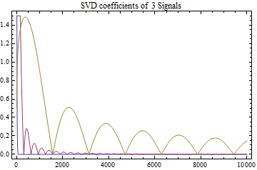
Figure 1: Left: SVD representation of a super-smooth (blue), a smooth (red) and a rough (olive) signal. Right: Relative efficiency for early stopping with m0=0m_{0}=0.

Let us exemplify the procedure by some Monte Carlo results. As a test bed we take the moderately ill-posed case λi=i−1/2\lambda_{i}=i^{-1/2} with noise level δ=0.01\delta=0.01 and dimension D=10 000D=10\,000. We consider early stopping at τ\tau with κ=D​δ2=1\kappa=D\delta^{2}=1.

In Figure 1 (left), we see the SVD representation of three signals: a very smooth signal μ⁡(1)\mu(1), a relatively smooth signal μ⁡(2)\mu(2) and a rough signal μ⁡(3)\mu(3), the attributes coming from the interpretation via the decay of Fourier coefficients. The corresponding weakly balanced oracle indices t𝔴t_{\mathfrak{w}} are (34,316,1356)(34,316,1356). The classical oracle indices in strong norm are (43,504,1331)(43,504,1331). Figure 1 (right) shows box-plots of the relative efficiency of early stopping in 1000 Monte Carlo replications defined as minm⁡𝔼⁡[∥μ^(m)−μ∥2]1/2/∥μ^(τ)−μ∥\min_{m}\E[\lVert\widehat{\mu}^{(m)}-\mu\rVert^{2}]^{1/2}/\lVert\widehat{\mu}^{(\tau)}-\mu\rVert, both for strong and weak norm. Ideally, the relative efficiency should concentrate around one. This is well achieved for the smooth and rough signals and even better than for the corresponding Landweber results in [2]. The super-smooth case with its very small oracle risk suffers from the variability within the residual and attains on average an efficiency of about 0.50.5, meaning that its root mean squared error is about twice as large as the oracle error. Let us mention that in unreported situations with higher ill-posedness the relative efficiency is similarly good or even better.

We are lead to consider the two-step procedure. According to Proposition 4.2 we have to choose an initial index somewhat larger than D\sqrt{D}. The factor in the choice there is very conservative due to non-tight concentration bounds. For the implementation we choose m0m_{0} such that for a zero signal μ=0\mu=0 the probability of {τ>m0}={Rm02>κ}\{\tau>m_{0}\}=\{R_{m_{0}}^{2}>\kappa\} is about 0.01, when applying a normal approximation, that is m0=⌊q0.99​2​D⌋+1=329m_{0}=\lfloor q_{0.99}\sqrt{2D}\rfloor+1=329 with the 99%99\%-percentile q0.99q_{0.99} of N⁡(0,1)N(0,1). In Figure 2(left) we see that with this choice for the super-smooth signal, 6 out of 1 000 MC realisations lead to τ>m0\tau>m_{0}, for the others we apply the second model selection step. The truncation for the smooth signal varies around m0m_{0}, and the second step is applied to about 50%50\% of the realisations. In the rough case, τ>m0\tau>m_{0} was always satisfied and no second model selection step was applied.

Refer to caption
Refer to caption
Figure 2: Left: truncation levels for early stopping with m0=0m_{0}=0 and the two-step procedures with m0=⌊q0.99​2​D⌋+1=329m_{0}=\lfloor q_{0.99}\sqrt{2D}\rfloor+1=329, AIC in weak and strong norm. Right: Relative efficiencies for the two-step procedure.

As model selection procedure we apply the AIC-criterion, based on the weak and strong empirical norm for the weak and strong norm criterion, respectively. The results are shown in Figure 2(right). We see that the efficiency for the super-smooth signal improves significantly (with the 6 outliers not being affected). The variability is still considerably higher than for the other two signals. This phenomenon is well known for unbiased risk estimation. Especially for more strongly ill-posed problems, one should penalise stronger, see the comparison with the risk hull approach in Cavalier and Golubev [7] and the numerical findings in Lucka et al. [14]. Here let us rather emphasize that a pure AIC-minimisation for the super-smooth signal gives exactly the same result, apart from the 6 outliers, but requires to calculate the AIC-criterion for D=10 000D=10\,000 indices in 1 000 MC iterations. The two-step procedure, even for known SVD, is about 30 times faster.

5 Appendix

5.1 Proof of Corollary 2.2

Proof.

For i0=⌊(2Cμ2CA)1/(2​p+1)(R−1δ)−2/(2β+2p+1)⌋i_{0}=\lfloor(2C_{\mu}^{2}C_{A})^{1/(2p+1)}(R^{-1}\delta)^{-2/(2\beta+2p+1)}\rfloor, we can choose c2c_{2} (in dependence of Cμ,CAC_{\mu},C_{A}) big enough so that our assumptions imply i0≤Di_{0}\leq D and

1−ℛ​(μ,τ)2Vi0+1≥1−Cμ2​CA​((R−1δ)−2/(2β+2p+1)i0+1)1+2​p≥12.1-\frac{{\cal R}(\mu,\tau)^{2}}{V_{i_{0}+1}}\geq 1-C_{\mu}^{2}C_{A}\Bigg(\frac{(R^{-1}\delta)^{-2/(2\beta+2p+1)}}{i_{0}+1}\Bigg)^{1+2p}\geq\frac{1}{2}.

Put μ¯i=μi\bar{\mu}_{i}=\mu_{i} for i≠i0+1i\not=i_{0}+1 and μ¯i0+1=12​R¯​(i0+1)−α\bar{\mu}_{i_{0}+1}=\tfrac{1}{2}\bar{R}(i_{0}+1)^{-\alpha}. Then μ¯∈Hα​(R¯,D)\bar{\mu}\in H^{\alpha}(\bar{R},D) follows from μ∈Hβ​(R,D)⊆Hα​(R,D)\mu\in H^{\beta}(R,D)\subseteq H^{\alpha}(R,D) and R¯≥2​R\bar{R}\geq 2R. The bias bound Bi02​(μ¯)≥14​R¯2​(i0+1)−2​αB_{i_{0}}^{2}(\bar{\mu})\geq\tfrac{1}{4}\bar{R}^{2}(i_{0}+1)^{-2\alpha} inserted in Proposition 2.1 yields the result. ∎

5.2 Proof of Lemma 2.3

Proof.

With Sm=δ2​∑i=1mλi−2​εi2S_{m}=\delta^{2}\sum_{i=1}^{m}\lambda_{i}^{-2}\varepsilon_{i}^{2} we obtain

ℛ​(μ,τ)2≥𝔼⁡[δ2​∑i=1τλi−2​εi2]≥𝔼⁡[𝟏​(τ≥m)​Sm].{\mathcal{R}}(\mu,\tau)^{2}\geq\mathbb{E}\Big[\delta^{2}\sum_{i=1}^{\tau}\lambda_{i}^{-2}\varepsilon_{i}^{2}\Big]\geq\mathbb{E}\Big[{\mathbf{1}(\tau\geq m)}S_{m}\Big].

By Lemma 1 in Laurent and Massart [12], for nonnegative weights aia_{i}, we have

P⁡(∑i=1Dai​(εi2−1)<−2​‖a‖​x)<e−x.P\Big(\sum_{i=1}^{D}a_{i}(\varepsilon_{i}^{2}-1)<-2\|a\|\sqrt{x}\Big)<e^{-x}. (5.1)

Picking a=δ2​(λ1−2,…,λm−2)a=\delta^{2}(\lambda_{1}^{-2},\ldots,\lambda_{m}^{-2}) and x=log⁡(5/4)x=\log(5/4) so that 2​x≤0.952\sqrt{x}\leq 0.95, with probability larger than 1−e−x=0.21-e^{-x}=0.2, it follows that

Sm≥𝔼⁡[Sm]−2​∥a∥​x≥δ220​∑i=1mλi−2=Vm20,S_{m}\geq\mathbb{E}\left[S_{m}\right]-2\lVert a\rVert\sqrt{x}\geq\frac{\delta^{2}}{20}\sum_{i=1}^{m}\lambda_{i}^{-2}=\frac{V_{m}}{20},

where we used ∥a∥≤∑i=1mai=𝔼⁡[Sm]=Vm\lVert a\rVert\leq\sum_{i=1}^{m}a_{i}=\mathbb{E}\left[S_{m}\right]=V_{m}  (observe that we could tighten the latter inequality significantly under some additional assumptions on the singular value decay). We now have

ℛ​(μ,τ)2\displaystyle{\mathcal{R}}(\mu,\tau)^{2} ≥𝔼⁡[𝟏​(τ≥m)​Sm]\displaystyle\geq\mathbb{E}\left[{\mathbf{1}(\tau\geq m)}S_{m}\right]
≥VmP({τ≥m}∩{Sm≥Vm/20})/20\displaystyle\geq V_{m}P(\left\{\tau\geq m\right\}\cap\left\{S_{m}\geq V_{m}/20\right\})/20
≥Vm​(1−P⁡(τ<m)−P⁡(Sm<Vm/20))/20\displaystyle\geq V_{m}\big(1-P(\tau<m)-P(S_{m}<V_{m}/20)\big)/20
≥Vm​(0.2−P⁡(τ<m))/20.\displaystyle\geq V_{m}\big(0.2-P(\tau<m)\big)/20.

We deduce from this that Vm≥200​ℛ​(μ,τ)2V_{m}\geq 200{\mathcal{R}}(\mu,\tau)^{2} implies P⁡(τ≥m)≤0.9P(\tau\geq m)\leq 0.9. ∎

5.3 A total variation bound for non-central χ2\chi^{2}-laws

5.1 Lemma.

Let ϑ=(ϑ1,…,ϑK)∈ℝK\vartheta=(\vartheta_{1},\ldots,\vartheta_{K})\in\R^{K} and ℙKϑ\PP_{K}^{\vartheta} be the non-central χ2\chi^{2}-law of Xϑ=∑k=1K(ϑk+Zk)2X_{\vartheta}=\sum_{k=1}^{K}(\vartheta_{k}+Z_{k})^{2} with ZkZ_{k} independent and standard Gaussian. Then, for ϑ,ϑ¯∈ℝK\vartheta,\bar{\vartheta}\in\R^{K} we have

∥ℙKϑ−ℙKϑ¯∥TV≤e​|∥ϑ∥2−∥ϑ¯∥2|+8/π​|∥ϑ∥−∥ϑ¯∥|π​K,\lVert\PP_{K}^{\vartheta}-\PP_{K}^{\bar{\vartheta}}\rVert_{TV}\leq e\frac{\lvert\lVert\vartheta\rVert^{2}-\lVert\bar{\vartheta}\rVert^{2}\rvert+\sqrt{8/\pi}\lvert\lVert\vartheta\rVert-\lVert\bar{\vartheta}\rVert\rvert}{\sqrt{\pi K}},

For ∥ϑ∥+∥ϑ¯∥≥8​e2​π−π​e≈5.248\lVert\vartheta\rVert+\lVert\bar{\vartheta}\rVert\geq\frac{\sqrt{8}e}{2\pi-\sqrt{\pi}e}\approx 5.248 this bound simplifies to

∥ℙKϑ−ℙKϑ¯∥TV≤2​|∥ϑ∥2−∥ϑ¯∥2|K.\lVert\PP_{K}^{\vartheta}-\PP_{K}^{\bar{\vartheta}}\rVert_{TV}\leq 2\frac{\lvert\lVert\vartheta\rVert^{2}-\lVert\bar{\vartheta}\rVert^{2}\rvert}{\sqrt{K}}.
Proof.

Writing ϑ=(ϑk),Z=(Zk)∈ℝk\vartheta=(\vartheta_{k}),Z=(Z_{k})\in\R^{k} we see by orthogonal transformation that Xϑ=∥ϑ∥2+2​⟨ϑ,Z⟩+∥Z∥2X_{\vartheta}=\lVert\vartheta\rVert^{2}+2\langle\vartheta,Z\rangle+\lVert Z\rVert^{2} equals in law Xϑ′=∥ϑ∥2+2​∥ϑ∥​Z1′+∥Z′∥2X^{\prime}_{\vartheta}=\lVert\vartheta\rVert^{2}+2\lVert\vartheta\rVert Z_{1}^{\prime}+\lVert Z^{\prime}\rVert^{2} with Z1′,…,ZK′∼N⁡(0,1)Z_{1}^{\prime},\ldots,Z_{K}^{\prime}\sim N(0,1) i.i.d. We can therefore first consider the conditional law ℚKϑ⁡(z)\QQ_{K}^{\vartheta}(z) of ℙKϑ\PP_{K}^{\vartheta} given {Z1′=z}\{Z_{1}^{\prime}=z\}, which is nothing but the χ2​(K−1)\chi^{2}(K-1)-distribution translated by ∥ϑ∥2+2​∥ϑ∥​z+z2\lVert\vartheta\rVert^{2}+2\lVert\vartheta\rVert z+z^{2}.

If fpf_{p} denotes the χ2​(p)\chi^{2}(p)-density, then we have for any t>0t>0 that fp​(x−t)>fp​(x)f_{p}(x-t)>f_{p}(x) holds iff x≥xt=t1−e−t/(p−2)x\geq x_{t}=\frac{t}{1-e^{-t/(p-2)}}. Thus, we obtain

∫0∞|fp​(x−t)−fp​(x)|​𝑑x= 2​∫0∞(fp​(x−t)−fp​(x))+​𝑑x=21−p/2Γ⁡(p/2)∫xt∞((1−t/x)p/2−1et/2−1)xp/2−1e−x/2dx=21−p/2Γ⁡(p/2)∫xt−txtx(p−2)/2e−x/2dx≤2(2−p)/2Γ⁡(p/2)t(p−2)(p−2)/2e−(p−2)/2,\,\int_{0}^{\infty}\lvert f_{p}(x-t)-f_{p}(x)\rvert\,dx\\ \begin{aligned} =&\,2\int_{0}^{\infty}\big(f_{p}(x-t)-f_{p}(x)\big)_{+}\,dx\\ =&\,\frac{2^{1-p/2}}{\Gamma(p/2)}\int_{x_{t}}^{\infty}\big((1-t/x)^{p/2-1}e^{t/2}-1\big)x^{p/2-1}e^{-x/2}dx\\ =&\,\frac{2^{1-p/2}}{\Gamma(p/2)}\int_{x_{t}-t}^{x_{t}}x^{(p-2)/2}e^{-x/2}dx\\ \leq&\,\frac{2^{(2-p)/2}}{\Gamma(p/2)}t(p-2)^{(p-2)/2}e^{-(p-2)/2},\end{aligned}

knowing that x=p−2x=p-2 is the mode of fpf_{p}. Stirling’s formula guarantees Γ⁡(x)≥2​π/x​(x/e)x\Gamma(x)\geq\sqrt{2\pi/x}(x/e)^{x} for all x>0x>0 such that the last expression is always bounded by t(πp)−1/2et(\pi p)^{-1/2}e. This yields

∥ℚKϑ(z)−ℚKϑ¯(z)∥TV≤e(πK)−1/2|∥ϑ∥2−∥ϑ¯∥2+2(∥ϑ∥−∥ϑ¯∥)z|.\lVert\QQ_{K}^{\vartheta}(z)-\QQ_{K}^{\bar{\vartheta}}(z)\rVert_{TV}\leq e(\pi K)^{-1/2}\big|\lVert\vartheta\rVert^{2}-\lVert\bar{\vartheta}\rVert^{2}+2(\lVert\vartheta\rVert-\lVert\bar{\vartheta}\rVert)z\big|.

Taking expectation with respect to Z1′∼N⁡(0,1)Z_{1}^{\prime}\sim N(0,1) we conclude

∥ℙKϑ−ℙKϑ¯∥TV≤e(πK)−1/2|∥ϑ∥−∥ϑ¯∥|𝔼[|∥ϑ∥+∥ϑ¯∥+2Z1′|].\lVert\PP_{K}^{\vartheta}-\PP_{K}^{\bar{\vartheta}}\rVert_{TV}\leq e(\pi K)^{-1/2}\big|\lVert\vartheta\rVert-\lVert\bar{\vartheta}\rVert\big|\E\big[\big|\lVert\vartheta\rVert+\lVert\bar{\vartheta}\rVert+2Z_{1}^{\prime}\big|\big].

Using the triangle inequality and 𝔼⁡[|Z1′|]=2/π\E[\lvert Z_{1}^{\prime}\rvert]=\sqrt{2/\pi}, the upper bound follows. ∎

5.4 Proof of Corollary 2.5

Proof.

Set μ¯i=μi\bar{\mu}_{i}=\mu_{i} for i≠i0+1i\not=i_{0}+1 and μ¯i0+12=μi0+12+14​R¯2​(i0+1)−2​α\bar{\mu}_{i_{0}+1}^{2}=\mu_{i_{0}+1}^{2}+\tfrac{1}{4}\bar{R}^{2}(i_{0}+1)^{-2\alpha} for some i0∈{1,…,D}i_{0}\in\{1,\ldots,D\}, so that μ¯∈Hα​(R¯,D)\bar{\mu}\in H^{\alpha}(\bar{R},D) and condition (a)(a) of Proposition 2.4 is satisfied. If

(b’): CA24R¯2(i0+1)−2​(α+p)≤0.025δ2D−i0\text{(b'): }\tfrac{C_{A}^{2}}{4}\bar{R}^{2}(i_{0}+1)^{-2(\alpha+p)}\leq 0.025\delta^{2}\sqrt{D-i_{0}}

holds, then condition (b) of Proposition 2.4 is ensured, whereas

(c’): R¯2(i0+1)−2​(α+p)≥2CA25.252δ2\text{(c'): }\bar{R}^{2}(i_{0}+1)^{-2(\alpha+p)}\geq 2C_{A}^{2}5.25^{2}\delta^{2}

implies condition (c) of Proposition 2.4. Finally, for

(d’): i0≥⌊(200(1+2p)CA2Cμ2)1/(2​p+1)(R2δ−2)1/(2​β+2​p+1)⌋,\text{(d'): }i_{0}\geq\lfloor(200(1+2p)C_{A}^{2}C_{\mu}^{2})^{1/(2p+1)}(R^{2}\delta^{-2})^{1/(2\beta+2p+1)}\rfloor,

we have Vi0+1≥200​ℛ​(μ,τ)2V_{i_{0}+1}\geq 200{\cal R}(\mu,\tau)^{2}. Hence, by Proposition 2.4, (b’)-(c’)-(d’) imply

ℛ​(μ¯,τ)2≥0.05​Bi02​(μ¯)≥0.054​R¯2​(i0+1)−2​α.{\cal R}(\bar{\mu},\tau)^{2}\geq 0.05B_{i_{0}}^{2}(\bar{\mu})\geq\tfrac{0.05}{4}\bar{R}^{2}(i_{0}+1)^{-2\alpha}.

For i0=⌊C0​max⁡((R¯2​δ−2/D)1/(2​α+2​p),(R2​δ−2)1/(2​β+2​p+1))⌋i_{0}=\big\lfloor C_{0}\max\big((\bar{R}^{2}\delta^{-2}/\sqrt{D})^{1/(2\alpha+2p)},(R^{2}\delta^{-2})^{1/(2\beta+2p+1)}\big)\big\rfloor with some suitably large constant C0>0C_{0}>0, depending only on Cμ,CA,pC_{\mu},C_{A},p, and for D≥2​i0D\geq 2i_{0}, conditions (b’) and (d’) are satisfied. To check condition (c’), a sufficient condition is i0+1≤(R¯2​δ−2/(56​CA2))1/(2​α+2​p)i_{0}+1\leq(\bar{R}^{2}\delta^{-2}/(56C_{A}^{2}))^{1/(2\alpha+2p)}. The first term in the maximum defining i0i_{0} satisfies this condition (here again using D≥2​i0D\geq 2i_{0}) provided R−1​δR^{-1}\delta is smaller than a suitable constant c2′c_{2}^{\prime} depending on CA,Cμ,α,pC_{A},C_{\mu},\alpha,p. The second term in the maximum defining i0i_{0} satisfies the sufficient condition

C0​(R2​δ−2)1/(2​β+2​p+1)≤C0​(R¯2​δ−2)1/(2​α+2​p+1)≤(R¯2​δ−2/(56​CA2))1/(2​α+2​p),C_{0}(R^{2}\delta^{-2})^{1/(2\beta+2p+1)}\leq C_{0}(\bar{R}^{2}\delta^{-2})^{1/(2\alpha+2p+1)}\leq(\bar{R}^{2}\delta^{-2}/(56C_{A}^{2}))^{1/(2\alpha+2p)},

again as soon as R−1​δR^{-1}\delta is smaller than a suitable constant c2′′c_{2}^{\prime\prime} depending on the same parameters as c2′c_{2}^{\prime}. Finally, putting c2=min⁡(c2′,c2′′,1)c_{2}=\min(c_{2}^{\prime},c_{2}^{\prime\prime},1) and unwrapping the condition D≥2​i0D\geq 2i_{0}, yields (using R​δ−1≥1R\delta^{-1}\geq 1) the sufficient condition D≥c3′​(R¯2​δ−2)1/(2​α+2​p+1/2)D\geq c_{3}^{\prime}(\bar{R}^{2}\delta^{-2})^{1/(2\alpha+2p+1/2)}, which is equivalent to the assumption D≥c3​tα−14,p,R¯​(δ)D\geq c_{3}t_{\alpha-\frac{1}{4},p,\bar{R}}(\delta) postulated in the statement, for suitable c3′,c3c_{3}^{\prime},c_{3} depending on Cμ,CA,α,pC_{\mu},C_{A},\alpha,p. This yields the result. ∎

5.5 Proof of Proposition 3.4

Proof.

By partial summation, we deduce from Bτ,λ2​(μ)>Bt∗,λ2​(μ)B_{\tau,\lambda}^{2}(\mu)>B_{t^{\ast},\lambda}^{2}(\mu), which implies τ≤⌊t∗⌋\tau\leq\lfloor t^{\ast}\rfloor:

𝔼⁡[(Bτ,λ2​(μ)−Bt∗,λ2​(μ))+]\displaystyle\E[(B_{\tau,\lambda}^{2}(\mu)-B_{t^{\ast},\lambda}^{2}(\mu))_{+}] =∑m=m0⌊t∗⌋(Bm,λ2​(μ)−Bt∗,λ2​(μ))​P​(τ=m)\displaystyle=\sum_{m=m_{0}}^{\lfloor t^{\ast}\rfloor}(B_{m,\lambda}^{2}(\mu)-B_{t^{\ast},\lambda}^{2}(\mu))P(\tau=m)
=∑m=m0⌊t∗⌋∑k=m⌊t∗⌋(Bk,λ2​(μ)−B(k+1)∧t∗,λ2​(μ))​P​(τ=m)\displaystyle=\sum_{m=m_{0}}^{\lfloor t^{\ast}\rfloor}\sum_{k=m}^{\lfloor t^{\ast}\rfloor}(B_{k,\lambda}^{2}(\mu)-B_{(k+1)\wedge t^{\ast},\lambda}^{2}(\mu))P(\tau=m)
=∑m=m0⌊t∗⌋(Bm,λ2​(μ)−B(m+1)∧t∗,λ2​(μ))​P​(τ≤m).\displaystyle=\sum_{m=m_{0}}^{\lfloor t^{\ast}\rfloor}(B_{m,\lambda}^{2}(\mu)-B_{(m+1)\wedge t^{\ast},\lambda}^{2}(\mu))P(\tau\leq m).

In the case t∗=m0t^{\ast}=m_{0} all expressions evaluate to zero because of τ≥t∗\tau\geq t^{\ast} and we suppose t∗>m0t^{\ast}>m_{0} from now on, so that (3.4) holds. For m0≤m<t∗m_{0}\leq m<t^{\ast} we have {τ≤m}={Rm2≤κ}\{\tau\leq m\}=\{R_{m}^{2}\leq\kappa\}, 𝔼⁡[Rm2]≥κ\E[R_{m}^{2}]\geq\kappa and by Lemma 1 in [12] (recall (5.1) in the proof of Lemma 2.3) together with P(Z<−x)≤e−x2/(2σ2)P(Z<-x)\leq e^{-x^{2}/(2\sigma^{2})} for Z∼N⁡(0,σ2)Z\sim N(0,\sigma^{2}), x≥0x\geq 0 we obtain the bound

P⁡(Rm2≤κ)=P⁡(∑i=m+1D(δ2​(εi2−1)+2​λi​μi​δ​εi)≤−(𝔼⁡[Rm2]−κ))\displaystyle P(R_{m}^{2}\leq\kappa)=P\Big(\sum_{i=m+1}^{D}\big(\delta^{2}(\varepsilon_{i}^{2}-1)+2\lambda_{i}\mu_{i}\delta\varepsilon_{i}\big)\leq-(\E[R_{m}^{2}]-\kappa)\Big)
≤P⁡(∑i=m+1Dδ2​(εi2−1)≤−𝔼⁡[Rm2]−κ2)+P⁡(∑i=m+1Dλi​μi​δ​εi≤−𝔼⁡[Rm2]−κ4)\displaystyle\leq P\Big(\sum_{i=m+1}^{D}\delta^{2}(\varepsilon_{i}^{2}-1)\leq-\frac{\E[R_{m}^{2}]-\kappa}{2}\Big)+P\Big(\sum_{i=m+1}^{D}\lambda_{i}\mu_{i}\delta\varepsilon_{i}\leq-\frac{\E[R_{m}^{2}]-\kappa}{4}\Big)
≤exp⁡(−(𝔼⁡[Rm2]−κ)216​δ4​(D−m))+exp⁡(−(𝔼⁡[Rm2]−κ)232​δ2​Bm,λ2​(μ))\displaystyle\leq\exp\Big(-\frac{(\E[R_{m}^{2}]-\kappa)^{2}}{16\delta^{4}(D-m)}\Big)+\exp\Big(-\frac{(\E[R_{m}^{2}]-\kappa)^{2}}{32\delta^{2}B_{m,\lambda}^{2}(\mu)}\Big)
≤F⁡(Bm,λ2​(μ)−Bt∗,λ2​(μ)),\displaystyle\leq F(B_{m,\lambda}^{2}(\mu)-B_{t^{\ast},\lambda}^{2}(\mu)),

where we use 𝔼⁡[Rm2]−κ≥Bm,λ2​(μ)−Bt∗,λ2​(μ)\E[R_{m}^{2}]-\kappa\geq B_{m,\lambda}^{2}(\mu)-B_{t^{\ast},\lambda}^{2}(\mu) for m<t∗m<t^{*} (see (3.3), (3.4)), and put

F⁡(z):=exp⁡(−z216​δ4​D)+exp⁡(−z232​δ2​(Bt∗,λ2​(μ)+z)),z≥0.F(z):=\exp\Big(-\frac{z^{2}}{16\delta^{4}D}\Big)+\exp\Big(-\frac{z^{2}}{32\delta^{2}(B_{t^{\ast},\lambda}^{2}(\mu)+z)}\Big),\quad z\geq 0.

We conclude by monotonicity of B∙,λ2​(μ)B_{{\scriptstyle\bullet},\lambda}^{2}(\mu) and FF via a Riemann-Stieltjes sum approximation:

𝔼⁡[(Bτ,λ2​(μ)−Bt∗,λ2​(μ))+]\displaystyle\E\big[\big(B_{\tau,\lambda}^{2}(\mu)-B_{t^{\ast},\lambda}^{2}(\mu)\big)_{+}\big]
≤∑m=m0⌊t∗⌋(Bm,λ2​(μ)−B(m+1)∧t∗,λ2​(μ))​F​(Bm,λ2​(μ)−Bt∗,λ2​(μ))\displaystyle\leq\sum_{m=m_{0}}^{\lfloor t^{\ast}\rfloor}(B_{m,\lambda}^{2}(\mu)-B_{(m+1)\wedge t^{\ast},\lambda}^{2}(\mu))F(B_{m,\lambda}^{2}(\mu)-B_{t^{\ast},\lambda}^{2}(\mu))
≤∫Bt∗,λ2​(μ)Bm0,λ2​(μ)F⁡(y−Bt∗,λ2​(μ))​𝑑y\displaystyle\leq\int_{B_{t^{\ast},\lambda}^{2}(\mu)}^{B_{m_{0},\lambda}^{2}(\mu)}F(y-B_{t^{\ast},\lambda}^{2}(\mu))\,dy
≤∫0∞F⁡(z)​𝑑z\displaystyle\leq\int_{0}^{\infty}F(z)\,dz
≤4​π​δ4​D+∫0Bt∗,λ2​(μ)exp⁡(−z264​δ2​Bt∗,λ2​(μ))​𝑑z+∫Bt∗,λ2​(μ)∞exp⁡(−z64​δ2)​𝑑z\displaystyle\leq\sqrt{4\pi\delta^{4}D}+\int_{0}^{B_{t^{\ast},\lambda}^{2}(\mu)}\exp\Big(-\frac{z^{2}}{64\delta^{2}B_{t^{\ast},\lambda}^{2}(\mu)}\Big)\,dz+\int_{B_{t^{\ast},\lambda}^{2}(\mu)}^{\infty}\exp\Big(-\frac{z}{64\delta^{2}}\Big)\,dz
≤4​π​δ4​D+16​π​δ2​Bt∗,λ2​(μ)+64​δ2\displaystyle\leq\sqrt{4\pi\delta^{4}D}+\sqrt{16\pi\delta^{2}B_{t^{\ast},\lambda}^{2}(\mu)}+64\delta^{2}
≤(17D+64)δ2+Bt∗,λ2(μ)D−1/2,\displaystyle\leq\big(17\sqrt{D}+64\big)\delta^{2}+B_{t^{\ast},\lambda}^{2}(\mu)D^{-1/2},

using 4πδBt∗,λ(μ)≤4πDδ2+D−1/2Bt∗,λ2(μ)4\sqrt{\pi}\delta B_{t^{\ast},\lambda}(\mu)\leq 4\pi\sqrt{D}\delta^{2}+D^{-1/2}B_{t^{\ast},\lambda}^{2}(\mu) by the binomial identity and 4​π+4​π≤17\sqrt{4\pi}+4\pi\leq 17 in the last line. ∎

5.6 Proof of Proposition 3.6

Proof.

By the Cauchy-Schwarz inequality and 𝔼⁡[εm4]1/2=3\E[\varepsilon_{m}^{4}]^{1/2}=\sqrt{3}, we have

𝔼⁡[(Sτ−S⌊t∗⌋+1)+]\displaystyle\E\Big[(S_{\tau}-S_{\lfloor t^{\ast}\rfloor+1})_{+}\Big] =δ2​∑m=⌊t∗⌋+2Dλm−2​𝔼⁡[εm2​𝟏​(τ≥m)]\displaystyle=\delta^{2}\sum_{m=\lfloor t^{\ast}\rfloor+2}^{D}\lambda_{m}^{-2}\E[\varepsilon_{m}^{2}{\bf 1}(\tau\geq m)]
≤3​δ2​∑m=⌊t∗⌋+2Dλm−2​P​(τ≥m)1/2.\displaystyle\leq\sqrt{3}\delta^{2}\sum_{m=\lfloor t^{\ast}\rfloor+2}^{D}\lambda_{m}^{-2}P(\tau\geq m)^{1/2}.

For m≥t∗+1≥m0+1m\geq t^{\ast}+1\geq m_{0}+1 we have {τ≥m}={Rm−12>κ}\{\tau\geq m\}=\{R_{m-1}^{2}>\kappa\}, 𝔼⁡[Rm−12]≤κ\E[R^{2}_{m-1}]\leq\kappa and by P(∑i=1Dai(εi2−1)>x)≤exp(−x2/(4∥a∥2+4xmaxiai))P(\sum_{i=1}^{D}a_{i}(\varepsilon_{i}^{2}-1)>x)\leq\exp\big(-x^{2}/(4\|a\|^{2}+4x\max_{i}a_{i})\big) for ai≥0a_{i}\geq 0 (Lemma 1 in [12]) together with P(Z>x)≤e−x2/(2σ2)P(Z>x)\leq e^{-x^{2}/(2\sigma^{2})} for Z∼N⁡(0,σ2)Z\sim N(0,\sigma^{2}), x≥0x\geq 0, we obtain the bound

P⁡(Rm−12>κ)=P⁡(∑i=mD(δ2​(εi2−1)+2​λi​μi​δ​εi)>κ−𝔼⁡[Rm−12])\displaystyle P(R_{m-1}^{2}>\kappa)=P\Big(\sum_{i=m}^{D}\big(\delta^{2}(\varepsilon_{i}^{2}-1)+2\lambda_{i}\mu_{i}\delta\varepsilon_{i}\big)>\kappa-\E[R_{m-1}^{2}]\Big)
≤P⁡(∑i=mDδ2​(εi2−1)≥κ−𝔼⁡[Rm−12]2)+P⁡(∑i=mDλi​μi​δ​εi≥κ−𝔼⁡[Rm−12]4)\displaystyle\leq P\Big(\sum_{i=m}^{D}\delta^{2}(\varepsilon_{i}^{2}-1)\geq\frac{\kappa-\E[R_{m-1}^{2}]}{2}\Big)+P\Big(\sum_{i=m}^{D}\lambda_{i}\mu_{i}\delta\varepsilon_{i}\geq\frac{\kappa-\E[R_{m-1}^{2}]}{4}\Big)
≤exp⁡(−(κ−𝔼⁡[Rm−12])216​δ4​(D−m+1)+8​δ2​(κ−𝔼⁡[Rm−12]))+exp⁡(−(κ−𝔼⁡[Rm−12])232​δ2​Bm−1,λ2​(μ)).\displaystyle\leq\exp\Big(-\frac{(\kappa-\E[R_{m-1}^{2}])^{2}}{16\delta^{4}(D-m+1)+8\delta^{2}(\kappa-\E[R_{m-1}^{2}])}\Big)+\exp\Big(-\frac{(\kappa-\E[R_{m-1}^{2}])^{2}}{32\delta^{2}B_{m-1,\lambda}^{2}(\mu)}\Big).

For the numerator, we use the lower bound

κ−𝔼⁡[Rm−12]≥κ−𝔼⁡[Rt∗2]+δ2​(m−1−t∗)≥δ2​(m−1−t∗).\kappa-\E[R_{m-1}^{2}]\geq\kappa-\E[R_{t^{\ast}}^{2}]+\delta^{2}(m-1-t^{\ast})\geq\delta^{2}(m-1-t^{\ast}).

For the denominators, we use 16​δ4​(D−m+1)+8​δ2​(κ−𝔼⁡[Rm−12])≤16​δ4​D+8​δ2​κ16\delta^{4}(D-m+1)+8\delta^{2}(\kappa-\E[R_{m-1}^{2}])\leq 16\delta^{4}D+8\delta^{2}\kappa for the first term and 32​δ2​Bm−1,λ2​(μ)≤32​δ2​Bt∗,λ2​(μ)≤32​δ2​κ32\delta^{2}B_{m-1,\lambda}^{2}(\mu)\leq 32\delta^{2}B_{t^{\ast},\lambda}^{2}(\mu)\leq 32\delta^{2}\kappa for the second term. We arrive at

𝔼⁡[(Sτ−S⌊t∗⌋+1)+]\displaystyle\E\Big[(S_{\tau}-S_{\lfloor t^{\ast}\rfloor+1})_{+}\Big] ≤2​3​δ2​∑m=⌊t∗⌋+2Dλm−2​exp⁡(−(m−1−t∗)216​D+32​κ​δ−2).\displaystyle\leq 2\sqrt{3}\delta^{2}\sum_{m=\lfloor t^{\ast}\rfloor+2}^{D}\lambda_{m}^{-2}\exp\Big(-\frac{(m-1-t^{\ast})^{2}}{16D+32\kappa\delta^{-2}}\Big).

We add 𝔼⁡[(S⌊t∗⌋+1−St∗)+]≤2​3​δ2​λ⌊t∗⌋+1−2\E[(S_{\lfloor t^{\ast}\rfloor+1}-S_{t^{\ast}})_{+}]\leq 2\sqrt{3}\delta^{2}\lambda_{\lfloor t^{\ast}\rfloor+1}^{-2} and note (Sτ−St∗)+≤SD(S_{\tau}-S_{t^{\ast}})_{+}\leq S_{D}, which gives the trivial bound 𝔼⁡[SD]=D​δ2\E[S_{D}]=D\delta^{2}. Under the polynomial eigenvalue decay this yields the bound

rV,τ≤23CA2(1+∑k≥0(t∗+1+k)2​pe−k2/(16D+32κδ−2))∧D.r_{V,\tau}\leq 2\sqrt{3}C_{A}^{2}\Big(1+\sum_{k\geq 0}(t^{\ast}+1+k)^{2p}e^{-k^{2}/(16D+32\kappa\delta^{-2})}\Big)\wedge D.

In the sequel ’≲\lesssim’, ’≳\gtrsim’ denote inequalities up to a factor only depending on pp. A Riemann sum approximation shows for any R>0R>0

∑k≥0e−k2/R\displaystyle\sum_{k\geq 0}e^{-k^{2}/R} ≤1+∫0∞e−x2/Rdx≲R.\displaystyle\leq 1+\int_{0}^{\infty}e^{-x^{2}/R}dx\lesssim\sqrt{R}.

Similarly, we obtain

∑k≥0k2​pe−k2/R\displaystyle\sum_{k\geq 0}k^{2p}e^{-k^{2}/R} ≤∫0∞(1+x)2​pe−x2/Rdx≲Rp+1/2.\displaystyle\leq\int_{0}^{\infty}(1+x)^{2p}e^{-x^{2}/R}dx\lesssim R^{p+1/2}.

This yields

rVτ≲CA2​((t∗)2​p​D+κ​δ−2+(D+κ​δ−2)p+1/2).r_{V_{\tau}}\lesssim C_{A}^{2}\Big((t^{\ast})^{2p}\sqrt{D+\kappa\delta^{-2}}+(D+\kappa\delta^{-2})^{p+1/2}\Big).

On the other hand, we have

Vt∗=δ2​(∑m=1⌊t∗⌋λm−2+(t∗−⌊t∗⌋)​λ⌊t∗⌋+1−2)≳δ2​CA−2​(t∗)2​p+1,V_{t^{\ast}}=\delta^{2}\Big(\sum_{m=1}^{\lfloor t^{\ast}\rfloor}\lambda_{m}^{-2}+(t^{\ast}-\lfloor t^{\ast}\rfloor)\lambda_{\lfloor t^{\ast}\rfloor+1}^{-2}\Big)\gtrsim\delta^{2}C_{A}^{-2}(t^{\ast})^{2p+1},

implying the result with a suitable constant CpC_{p}. ∎

5.7 Proof of Proposition 4.2

Proof.

In this proof ’≲\lesssim’ denotes an inequality holding up to factors depending only on pp, CAC_{A}, CκC_{\kappa} and C2C_{2}; similarly, ’∼\sim’ denotes a two-sided inequality holding up to factors depending on these parameters. In the case t𝔰>m0t_{\mathfrak{s}}>m_{0} we use the independence of τ\tau from μ^(0),…​μ^(m0)\widehat{\mu}^{(0)},\ldots\widehat{\mu}^{(m_{0})} by Lemma 4.1 to obtain

𝔼⁡[∥μ^(ρ)−μ∥2​𝟏​(τ=m0)]\displaystyle\E[\lVert\widehat{\mu}^{(\rho)}-\mu\rVert^{2}{\bf 1}(\tau=m_{0})] =𝔼⁡[∥μ^(m^)−μ∥2]​P​(τ=m0)\displaystyle=\E[\lVert\widehat{\mu}^{(\widehat{m})}-\mu\rVert^{2}]P(\tau=m_{0})
≤C2​(𝔼⁡[∥μ^(m0)−μ∥2]+δ2)​P​(τ=m0)\displaystyle\leq C_{2}\Big(\E[\lVert\widehat{\mu}^{(m_{0})}-\mu\rVert^{2}]+\delta^{2}\Big)P(\tau=m_{0})
=C2​(𝔼⁡[∥μ^(τ)−μ∥2​𝟏​(τ=m0)]+δ2​P​(τ=m0)).\displaystyle=C_{2}\Big(\E[\lVert\widehat{\mu}^{(\tau)}-\mu\rVert^{2}{\bf 1}(\tau=m_{0})]+\delta^{2}P(\tau=m_{0})\Big).

On {τ>m0}\{\tau>m_{0}\} we have ρ=τ\rho=\tau and we apply Theorem 3.8 with t𝔰≥m0>Dt_{\mathfrak{s}}\geq m_{0}>\sqrt{D} to get

𝔼⁡[∥μ^(ρ)−μ∥2​𝟏​(τ>m0)]≤𝔼⁡[∥μ^(τ)−μ∥2]≲𝔼⁡[∥μ^(t𝔰)−μ∥2].\E[\lVert\widehat{\mu}^{(\rho)}-\mu\rVert^{2}{\bf 1}(\tau>m_{0})]\leq\E[\lVert\widehat{\mu}^{(\tau)}-\mu\rVert^{2}]\lesssim\E[\lVert\widehat{\mu}^{(t_{\mathfrak{s}})}-\mu\rVert^{2}].

Because of t𝔰>m0t_{\mathfrak{s}}>m_{0} we have 𝔼⁡[∥μ^(t𝔰)−μ∥2]≤2​mint∈[0,D]​𝔼⁡[∥μ^(t)−μ∥2]\E[\lVert\widehat{\mu}^{(t_{\mathfrak{s}})}-\mu\rVert^{2}]\leq 2\min_{t\in[0,D]}\E[\lVert\widehat{\mu}^{(t)}-\mu\rVert^{2}]. This gives the result in this case.

Next, consider the case t𝔰=m0t_{\mathfrak{s}}=m_{0} where Bm02​(μ)≤Vm0B_{m_{0}}^{2}(\mu)\leq V_{m_{0}}. Then the estimator μ^(m𝔰)\widehat{\mu}^{(m_{\mathfrak{s}})} with m𝔰∈{0,1,…,m0}m_{\mathfrak{s}}\in\{0,1,\ldots,m_{0}\} from (1.7) satisfies

𝔼⁡[∥μ^(m𝔰)−μ∥2]≤2​maxi​λi2λi+12​minm∈{0,…,D}⁡𝔼⁡[∥μ^(m)−μ∥2],\E\big[\lVert\widehat{\mu}^{(m_{\mathfrak{s}})}-\mu\rVert^{2}\big]\leq 2\max_{i}\frac{\lambda_{i}^{2}}{\lambda_{i+1}^{2}}\min_{m\in\{0,\ldots,D\}}\E\big[\lVert\widehat{\mu}^{(m)}-\mu\rVert^{2}\big],

noting that the factor maxi⁡λi2/λi+12\max_{i}\lambda_{i}^{2}/\lambda_{i+1}^{2} comes from the discretisation m𝔰m_{\mathfrak{s}} of the balanced oracle and is bounded by CA4​22​p≲1C_{A}^{4}2^{2p}\lesssim 1. Given the independence of τ\tau from {μ^(0),…,μ^(m0)}\{\widehat{\mu}^{(0)},\ldots,\widehat{\mu}^{(m_{0})}\} by Lemma 4.1 and the properties of the model selector m^\widehat{m}, we have

E⁡[∥μ^(ρ)−μ∥2​𝟏​(τ=m0)]\displaystyle E[\lVert\widehat{\mu}^{(\rho)}-\mu\rVert^{2}{\bf 1}(\tau=m_{0})] ≤C2​(𝔼⁡[∥μ^(m𝔰)−μ∥2]+δ2)\displaystyle\leq C_{2}\Big(\E[\lVert\widehat{\mu}^{(m_{\mathfrak{s}})}-\mu\rVert^{2}]+\delta^{2}\Big)
≲minm∈{0,…,D}⁡𝔼⁡[∥μ^(m)−μ∥2]+δ2.\displaystyle\lesssim\min_{m\in\{0,\ldots,D\}}\E[\lVert\widehat{\mu}^{(m)}-\mu\rVert^{2}]+\delta^{2}.

For m𝔰∈[m0/2,m0]m_{\mathfrak{s}}\in[m_{0}/2,m_{0}]

𝔼⁡[∥μ^(m0)−μ∥2]≤Bm𝔰2​(μ)+Vm0≲𝔼⁡[∥μ^(m𝔰)−μ∥2]\E[\lVert\widehat{\mu}^{(m_{0})}-\mu\rVert^{2}]\leq B_{m_{\mathfrak{s}}}^{2}(\mu)+V_{m_{0}}\lesssim\E[\lVert\widehat{\mu}^{(m_{\mathfrak{s}})}-\mu\rVert^{2}]

follows from Vm0∼δ2​m02​p+1∼Vm𝔰V_{m_{0}}\thicksim\delta^{2}m_{0}^{2p+1}\thicksim V_{m_{\mathfrak{s}}}. By Theorem 3.8 with t𝔰=m0t_{\mathfrak{s}}=m_{0} this gives

𝔼⁡[∥μ^(ρ)−μ∥2​𝟏​(τ>m0)]\displaystyle\E[\lVert\widehat{\mu}^{(\rho)}-\mu\rVert^{2}{\bf 1}(\tau>m_{0})] ≲𝔼⁡[∥μ^(m0)−μ∥2]≲𝔼⁡[∥μ^(m𝔰)−μ∥2]\displaystyle\lesssim\E[\lVert\widehat{\mu}^{(m_{0})}-\mu\rVert^{2}]\lesssim\E[\lVert\widehat{\mu}^{(m_{\mathfrak{s}})}-\mu\rVert^{2}]
≲minm∈{0,…,D}⁡𝔼⁡[∥μ^(m)−μ∥2].\displaystyle\lesssim\min_{m\in\{0,\ldots,D\}}\E[\lVert\widehat{\mu}^{(m)}-\mu\rVert^{2}].

For m𝔰<m0/2m_{\mathfrak{s}}<m_{0}/2 we obtain by {τ>m0}={Rm02>κ}\{\tau>m_{0}\}=\{R_{m_{0}}^{2}>\kappa\}, Sτ≤SDS_{\tau}\leq S_{D}, Bτ2​(μ)≤Bm02​(μ)B_{\tau}^{2}(\mu)\leq B_{m_{0}}^{2}(\mu) and the Cauchy-Schwarz inequality:

𝔼⁡[∥μ^(ρ)−μ∥2​𝟏​(τ>m0)]\displaystyle\E[\lVert\widehat{\mu}^{(\rho)}-\mu\rVert^{2}{\bf 1}(\tau>m_{0})] ≤𝔼⁡[(Bm02​(μ)+SD)​𝟏​(Rm02>κ)]\displaystyle\leq\E[(B_{m_{0}}^{2}(\mu)+S_{D}){\bf 1}(R_{m_{0}}^{2}>\kappa)]
≤Bm02​(μ)​P​(Rm02>κ)+𝔼⁡[SD2]1/2​P​(Rm02>κ)1/2.\displaystyle\leq B_{m_{0}}^{2}(\mu)P(R_{m_{0}}^{2}>\kappa)+\E[S_{D}^{2}]^{1/2}P(R_{m_{0}}^{2}>\kappa)^{1/2}.

We have Bm02​(μ)≤Bm𝔰2​(μ)≤VDB_{m_{0}}^{2}(\mu)\leq B_{m_{\mathfrak{s}}}^{2}(\mu)\leq V_{D} and 𝔼⁡[SD2]1/2≲𝔼⁡[SD]=VD\E[S_{D}^{2}]^{1/2}\lesssim\E[S_{D}]=V_{D} (by comparison of Gaussian moments), so that

𝔼⁡[∥μ^(ρ)−μ∥2​𝟏​(τ>m0)]≲VD​P​(Rm02>κ)1/2∼δ2​DP​(Rm02>κ)1/2.\E[\lVert\widehat{\mu}^{(\rho)}-\mu\rVert^{2}{\bf 1}(\tau>m_{0})]\lesssim V_{D}P(R_{m_{0}}^{2}>\kappa)^{1/2}\thicksim\delta^{2}DP(R_{m_{0}}^{2}>\kappa)^{1/2}.

Observing m𝔴:=min⁡{m≥0|Bm,λ2​(μ)≤Vm,λ}≤m𝔰<m0/2m_{\mathfrak{w}}:=\min\{m\geq 0\,|\,B_{m,\lambda}^{2}(\mu)\leq V_{m,\lambda}\}\leq m_{\mathfrak{s}}<m_{0}/2 we obtain

𝔼⁡[Rm02]−κ=Bm0,λ2​(μ)−Vm0,λ≤Bm𝔴,λ2​(μ)−m0​δ2≤−(m0/2)​δ2.\E[R_{m_{0}}^{2}]-\kappa=B_{m_{0},\lambda}^{2}(\mu)-V_{m_{0},\lambda}\leq B_{m_{\mathfrak{w}},\lambda}^{2}(\mu)-m_{0}\delta^{2}\leq-(m_{0}/2)\delta^{2}.

As in the proof of Proposition 3.6 we therefore find

P⁡(Rm02>κ)≤exp⁡(−m0264​(D−m0)+16​m0)+exp⁡(−m02​δ2128​Bm0,λ2​(μ)).P(R_{m_{0}}^{2}>\kappa)\leq\exp\Big(-\frac{m_{0}^{2}}{64(D-m_{0})+16m_{0}}\Big)+\exp\Big(-\frac{m_{0}^{2}\delta^{2}}{128B_{m_{0},\lambda}^{2}(\mu)}\Big).

By the choice of m0m_{0} and Bm0,λ2​(μ)≤Bm0/2,λ2​(μ)≤(m0/2)​δ2B_{m_{0},\lambda}^{2}(\mu)\leq B_{m_{0}/2,\lambda}^{2}(\mu)\leq(m_{0}/2)\delta^{2}, using D≥3⇒log⁡D≥1D\geq 3\Rightarrow\log D\geq 1, we deduce

P⁡(Rm02>κ)≤2​exp⁡(−2​log⁡D)=2​D−2.P(R_{m_{0}}^{2}>\kappa)\leq 2\exp\big(-2\log D\big)=2D^{-2}.

Insertion of this bound yields 𝔼⁡[∥μ^(ρ)−μ∥2​𝟏​(τ>m0)]≲δ2\E[\lVert\widehat{\mu}^{(\rho)}-\mu\rVert^{2}{\bf 1}(\tau>m_{0})]\lesssim\delta^{2}, which accomplishes the proof for the case t𝔰=m0t_{\mathfrak{s}}=m_{0} and m𝔰≤m0/2m_{\mathfrak{s}}\leq m_{0}/2. ∎

Acknowledgement

Very instructive hints and questions by Thorsten Hohage, Alexander Goldenshluger, Peter Mathé and two anonymous referees are gratefully acknowledged. This research was supported by the DFG via SFB 1294 Data Assimilation and via Research Unit 1735 Structural Inference in Statistics, which has made possible a six months visit by MH to Humboldt-Universität zu Berlin.

References

  • [1] N. Bissantz, T. Hohage, A. Munk, and F. Ruymgaart. Convergence rates of general regularization methods for statistical inverse problems and applications. SIAM Journal on Numerical Analysis, 45:2610–2636, 2007.
  • [2] G. Blanchard, M. Hoffmann, and M. Reiß. Optimal adaptation for early stopping in statistical inverse problems. SIAM Journal of Uncertainty Quantification, 6:1043–1075, 2018.
  • [3] G. Blanchard and P. Mathé. Discrepancy principle for statistical inverse problems with application to conjugate gradient iteration. Inverse Problems, 28:pp. 115011, 2012.
  • [4] P. Bühlmann and T. Hothorn. Boosting algorithms: Regularization, prediction and model fitting. Statistical Science, pages 477–505, 2007.
  • [5] L. Cavalier. Inverse problems in statistics. In Inverse problems and high-dimensional estimation, pages 3–96. Lecture Notes in Statistics 203, Springer, 2011.
  • [6] L. Cavalier, G.K. Golubev D. Picard, and A.B. Tsybakov. Oracle inequalities for inverse problems. Annals of Statistics, 30:843–874, 2002.
  • [7] L. Cavalier and Y. Golubev. Risk hull method and regularization by projections of ill-posed inverse problems. Annals of Statistics, 34:1653–1677, 2006.
  • [8] E. Chernousova, Y. Golubev, and E. Krymova. Ordered smoothers with exponential weighting. Electronic Journal of Statistics, 7:2395–2419, 2013.
  • [9] A. Cohen, M. Hoffmann, and M. Reiß. Adaptive wavelet Galerkin methods for linear inverse problems. SIAM Journal on Numerical Analysis, 42(4):1479–1501, 2004.
  • [10] H. Engl, M. Hanke, and A. Neubauer. Regularization of Inverse Problems. Kluwer Academic Publishers, London, 1996.
  • [11] Y. Ingster and I. Suslina. Nonparametric goodness-of-fit testing under Gaussian models. Lecture Notes in Statistics 169, Springer, 2012.
  • [12] B. Laurent and P. Massart. Adaptive estimation of a quadratic functional by model selection. The Annals of Statistics, 28:1302–1338, 2000.
  • [13] O. Lepski. Some new ideas in nonparametric estimation. arXiv:1603.03934, 2016.
  • [14] F. Lucka, K. Proksch, C. Brune, N. Bissantz, M. Burger, H. Dette, and F. Wübbeling. Risk estimators for choosing regularization parameters in ill-posed problems - properties and limitations. e-print, arXiv:1701.04970, 2017.
  • [15] P. Mathé and S. V. Pereverzev. Geometry of linear ill-posed problems in variable hilbert scales. Inverse problems, 19(3):789, 2003.
  • [16] G. Raskutti, M. Wainwright, and B. Yu. Early stopping and non-parametric regression: An optimal data-dependent stopping rule. Journal of Machine Learning Research, 15:335–366, 2014.
  • [17] Y. Saad. Numerical Methods for Large Eigenvalue Problems: Revised Edition. Society for Industrial and Applied Mathematics (SIAM), 2011.
  • [18] A. B. Tsybakov. Introduction to nonparametric estimation. Springer Series in Statistics. Springer, New York, 2009.
  • [19] G. Wahba. Practical approximate solutions to linear operator equations when the data are noisy. SIAM Journal on Numerical Analysis, 14(4):651–667, 1977.
  • [20] Y. Yao, L. Rosasco, and A. Caponnetto. On early stopping in gradient descent learning. Constructive Approximation, 26(2):289–315, 2007.