Generalized Water-filling for Source-aware Energy-efficient SRAMsThanks: This work was supported in part by Systems on Nanoscale Information fabriCs (SONIC), one of the six SRC STARnet Centers, sponsored by MARCO and DARPA.

Yongjune Kim, Mingu Kang, Lav R. Varshney, and Naresh R. Shanbhag Affiliation: Affiliation: Coordinated Science Laboratory, University of Illinois at Urbana–Champaign
Urbana, IL, USA
Email: {yongjune, mkang17, varshney, shanbhag}@illinois.edu Affiliation:

Abstract

Conventional low-power static random access memories (SRAMs) reduce read energy by decreasing the bit-line voltage swings uniformly across the bit-line columns. This is because the read energy is proportional to the bit-line swings. On the other hand, bit-line swings are limited by the need to avoid decision errors especially in the most significant bits. We propose a principled approach to determine optimal non-uniform bit-line swings by formulating convex optimization problems. For a given constraint on mean squared error of retrieved words, we consider criteria to minimize energy (for low-power SRAMs), maximize speed (for high-speed SRAMs), and minimize energy-delay product. These optimization problems can be interpreted as classical water-filling, ground-flattening and water-filling, and sand-pouring and water-filling, respectively. By leveraging these interpretations, we also propose greedy algorithms to obtain optimized discrete swings. Numerical results show that energy-optimal swing assignment reduces energy consumption by half at a peak signal-to-noise ratio of 30dB for an 8-bit accessed word. The energy savings increase to four times for a 16-bit accessed word.

I Introduction

Von Neumann computing architectures separate memory units from computing units so there is frequent data access that consumes enormous energy. Since static random access memories (SRAMs) access requires more energy than arithmetic operations [1], SRAM access energy accounts for the significant part of the total energy consumption in many information processing circuits [2, 3, 4, 5, 6]. Thus, it is important to reduce the energy consumption of SRAM access. The basic way to reduce the access energy is to decrease either supply voltages or bit-line (BL) swings, which increases vulnerability to variations and noise. If we reduce supply voltages or BL swings across all BL columns [7, 8], then bit error rates (BERs) of all bit positions increase equally.

In many applications including signal processing and machine learning (ML) tasks, however, the impact of bit errors depends on bit position. For example, errors in the most significant bits (MSBs) of image pixels degrade overall image quality much more than errors in the least significant bits (LSBs). Likewise, an MSB error can cause a catastrophic loss in the inference accuracy of ML applications.

Until now, the following techniques have been proposed to address the different impacts of each bit position for energy efficiency:

1.

Storing the MSBs in more robust bit cells and the LSBs in less robust cells [9, 10],
2.

Applying higher supply voltage for the MSBs and lower supply voltage for the LSBs [11, 12, 13],
3.

Unequal error protection (UEP) by error control codes (ECCs) [14, 15],
4.

LSB dropping (dropping the LSBs at the cost of reduced arithmetic precision) [16, 17, 18].

The first approach requires costly bit cells redesign and manual array reorganization. Also, the bit cells are fixed at design time, so it is unable to dynamically track the time-varying fidelity requirement [18]. The second approach employs different supply voltages for each bit position, which significantly complicates the power routing network. Practical implementations only allow a few supply voltage levels [12, 13]. Fine-grained UEP [14, 15] requires complicated hardware implementations and dynamic change of protection is limited. LSB dropping [16, 17, 18] enables dynamic fidelity control by changing the number of dropped LSBs. Note that UEP and LSB dropping allow two levels of granularity (protected/unprotected or dropped/undropped) for each bit position.

In [17, 18], selective ECCs were proposed by combining UEP and LSB dropping. Since parity bits are stored in dropped LSB-cells, the encoded data has the same length as the uncoded data. In [19], the authors proposed adaptive coding techniques for different computations on the data read from faulty memories.

This paper presents an information-theoretic approach to determine the optimal BL swing assignments. For a given constraint on mean squared error (MSE) of retrieved words, we formulate convex optimization problems whose objectives are as follows:

C1.

Minimize energy (low-power SRAMs),
C2.

Maximize speed (high-speed SRAMs),
C3.

Minimize energy-delay product (EDP).

Solutions to these convex problems yield optimal performance that is theoretically attainable. By casting read access for SRAMs as communication over parallel channels, we investigate the fundamental trade-offs between physical resources (energy, delay, and EDP) and a fidelity (MSE) constraint.

In addition, we provide generalized water-filling interpretations for our optimal solutions. This follows since accessing a $B$ -bit word is equivalent to communicating information through $B$ parallel channels. In classical water-filling, the ground represents the noise levels of parallel channels [20, 21]. On the other hand, the importance of each bit position determines the ground level in our optimization problems. Each optimization problem has its own interpretation depending on its objective function: water-filling (C1), ground-flattening and water-filling (C2), and sand-pouring and water-filling (C3), respectively. We also observe interesting connections between our problems and variants on water-filling such as constant-power water-filling [22, 23] and mercury/water-filling [24]. Also, we show that the proposed optimization techniques can be extended to a wide range of sources and noise models.

Furthermore, we propose an SRAM circuit architecture to assign non-uniform bit-level swings. The proposed architecture separates the data for each bit position in different SRAM subarrays by interleaving. The proposed architecture enables fine-grained and dynamic control of bit-level swings depending on time-varying fidelity requirements with little circuit complexity overhead. Also, we propose greedy algorithms to optimize swing values drawn from a discrete set due to circuit implementation limitations. Generalized water-filling interpretations and Karush-Kuhn-Tucker (KKT) conditions are leveraged to develop these discrete optimization algorithms.

The rest of this paper is organized as follows. Section II introduces key metrics of energy, delay, and fidelity. Section III formulates the convex optimization problems to determine the optimum bit-level swings and provides generalized water-filling interpretations. Section IV shows that the proposed optimization techniques can be extended to various source and noise models. Section V investigates the SRAM architecture and develops greedy algorithms to optimize discrete swings. Section VI gives numerical results and Section VII concludes.

II SRAM Metrics for Resource and Fidelity

Fig. 1: A typical

N_{\text{BL}}\times N_{\text{WL}}

SRAM block (

N_{\text{BL}}=6

and

N_{\text{WL}}=5

The total energy in an SRAM read access is given by

\mathsf{E}_{\text{total}}=\mathsf{E}_{\text{array}}+\mathsf{E}_{\text{peri}}+\mathsf{E}_{\text{leakage}}

(1)

where $\mathsf{E}_{\text{array}}$ and $\mathsf{E}_{\text{peri}}$ denote the dynamic energy consumption from the SRAM bit cell array and the peripheral circuitry, respectively, and $\mathsf{E}_{\text{leakage}}$ represents the energy loss due to leakage. $\mathsf{E}_{\text{array}}$ is the dominant component of energy consumption in high-density SRAMs during normal read operations [8, 25, 3]. Hence, we focus on $\mathsf{E}_{\text{array}}$ , which is given by

\displaystyle\mathsf{E}_{\text{array}}

\displaystyle\propto N_{\text{BL}}N_{\text{WL}}C_{\text{bit}}V_{\text{dd}}\Delta

(2)

where $N_{\text{BL}}$ and $N_{\text{WL}}$ are the numbers of bit-lines (BLs) and word-lines (WLs) in a memory bank, respectively. $C_{\text{bit}}$ is the BL capacitance per bit cell and $V_{\text{dd}}$ is the supply voltage. Also, $\Delta$ denotes the BL voltage swing in read access. As shown in Fig. 1, the voltage swing $\Delta$ is the voltage difference between BL and BL-bar (BLB). This voltage difference occurs because either BL or BLB is discharged according to the stored bit. A sense amplifier detects which line (BL or BLB) has the higher voltage and decides whether the corresponding bit cell stores 1 or 0.

The swing $\Delta$ can be controlled by changing the WL pulse-width (i.e., WL activation time) $T_{\text{WL}}$ since

\Delta=\frac{I_{c}}{N_{\text{WL}}C_{\text{bit}}}\cdot T_{\text{WL}}

(3)

where $I_{c}$ is the discharge current of BL corresponding to the accessed bit cell [8]. From (2) and (3), we can observe that $\mathsf{E}_{\text{array}}$ is directly proportional to $T_{\text{WL}}$ . Also, $T_{\text{WL}}$ has a direct impact on the read access time [8, 26].

Since larger voltage swing $\Delta$ improves noise margin, there are trade-off relations between reliability, energy, and delay. These relations will be explained in the following subsections.

II-A Resource Metrics for Accessing $B$ -bit Word: Energy, Delay, and EDP

We define resource metrics for energy, delay, and EDP for accessing a $B$ -bit word. First, read access energy can be defined as follows.

Definition 1

The read energy to access a $B$ -bit word is

\mathsf{E}(\mathbf{\Delta})=\sum_{b=0}^{B-1}{\Delta_{b}}=\mathbf{1}^{\mathsf{T}}\mathbf{\Delta}

(4)

where $\mathbf{1}$ denotes the all-one vector and the superscript $\mathsf{T}$ denotes transpose. Note that $\mathbf{\Delta}=\left(\Delta_{0},\ldots,\Delta_{B-1}\right)$ where $\Delta_{b}$ denotes the swing for the $b$ th bit position in a $B$ -bit word. Note that $\mathsf{E}(\mathbf{\Delta})$ represents $\mathsf{E}_{\text{array}}$ in (1).

Definition 2

The maximum swing corresponding to a $B$ -bit word is

\rho=\max(\mathbf{\Delta})=\max\left\{\Delta_{0},\ldots,\Delta_{B-1}\right\}.

(5)

If we allot non-uniform swings for each bit position, the access time for a $B$ -bit word depends on $T_{\text{max}}=\max\{T_{\text{WL},0},\ldots,T_{\text{WL},B-1}\}$ where $T_{\text{WL},b}$ denotes the WL pulse-width for the $b$ th bit position. Note that $T_{\text{max}}$ is the pulse-width corresponding to the maximum swing $\rho$ because of (3). Hence, the maximum swing $\rho$ is a proper metric to be minimized to maximize read speed.

The EDP is considered to be a fundamental metric as it captures the trade-off between energy and delay [27, 28]. We define the EDP for accessing a $B$ -bit word based on Definitions 1 and 2.

Definition 3

The EDP to access a $B$ -bit word is

\mathsf{EDP}(\mathbf{\Delta})=\mathsf{E}(\mathbf{\Delta})\cdot\rho=\mathbf{1}^{\mathsf{T}}\mathbf{\Delta}\cdot\rho.

(6)

II-B Fidelity Metric for Accessing $B$ -bit Word: MSE

We will define a fidelity metric for accessing a $B$ -bit word. Suppose that a $B$ -bit word $x=(x_{0},\ldots,x_{B-1})$ is stored in SRAM cells, where $x_{0}$ and $x_{B-1}$ are the LSB and MSB, respectively. Note that $x$ can be represented by

x=\sum_{b=0}^{B-1}{2^{b}x_{b}}

(7)

where $x_{b}\in\left\{0,1\right\}$ and $x\in\left[0,2^{B}-1\right]$ (for integers $i$ and $j$ such that $i<j$ , $\left[i,j\right]=\left\{i,\ldots,j\right\}$ ). Also, $\widehat{x}=(\widehat{x}_{0},\ldots,\widehat{x}_{B-1})$ denotes the retrieved $B$ -bit word. A decision error flips the original bit $x_{b}$ as follows:

\widehat{x}_{b}=x_{b}\oplus\epsilon_{b}

(8)

where $\oplus$ denotes XOR operator and $\epsilon_{b}=1$ denotes a bit error in $b$ th bit position. The decimal representation of the retrieved word is $\widehat{x}=\sum_{b=0}^{B-1}{2^{b}\widehat{x}_{b}}$ . The decimal error $e$ is given by

e=\widehat{x}-x=\sum_{B=0}^{B-1}{2^{b}e_{b}}

(9)

where $e_{b}=\widehat{x}_{b}-x_{b}\in\left\{-1,0,1\right\}$ .

Remark 4

The decimal error $e=(e_{0},\ldots,e_{B-1})$ depends on $x_{b}$ as well as $\epsilon_{b}$ . Suppose that $\mathbf{\epsilon}=(1,0,0,1)$ . If $x=(1,0,0,1)=9$ , then $\widehat{x}=(0,0,0,0)=0$ , i.e., $e=(-1,0,0,-1)=-9$ . If $x=(0,1,1,0)=6$ , then $\widehat{x}=(1,1,1,1)=15$ and $e=(1,0,0,1)=9$ .

Since major noise sources of SRAMs are well modeled as Gaussian distributions [29, 30, 31, 32], the error probability of the $b$ th bit position is given by

p_{b}=\Pr\left(\epsilon_{b}=1\right)=Q\left(\frac{\Delta_{b}}{\sigma}\right)

(10)

where $\Delta_{b}$ and $\sigma^{2}$ denote the swing of $b$ th bit position and the noise variance in the corresponding BL, respectively. Note that $Q(x)=\int_{x}^{\infty}{\frac{1}{\sqrt{2\pi}}\exp{\left(-\frac{t^{2}}{2}\right)dt}}$ . By increasing $\Delta_{b}$ in (10), we can reduce $p_{b}$ . However, larger $\Delta_{b}$ implies more energy consumption and slower speed (see Definitions 1 and 2).

To measure memory retrieval reliability, bit error probability (10) is not appropriate for many applications, since it does not distinguish the differential impact of MSB and LSB errors. Hence, we use the MSE as a fidelity metric.

Definition 5

The MSE of $x$ is given by

\mathsf{MSE}(x)=\mathbb{E}\left[(\widehat{x}-x)^{2}\right]=\mathbb{E}\left[e^{2}\right].

(11)

Lemma 6

For a uniformly distributed $x$ , $\mathsf{MSE}(x)$ is given by

\mathsf{MSE}(x)=\mathsf{MSE}(\mathbf{\Delta})=\sum_{b=0}^{B-1}{4^{b}Q\left(\frac{\Delta_{b}}{\sigma}\right)}.

(12)

Proof:

If $x$ is uniformly distributed, the $x_{b}$ s are independent and identically distributed (i.i.d.) and follow the Bernoulli distribution $\mathsf{Ber}\left(\frac{1}{2}\right)$ . The MSE of $x$ is given by

	$\displaystyle\mathsf{MSE}(x)$	$\displaystyle=\mathbb{E}\left[\left(\sum_{B=0}^{B-1}{2^{b}e_{b}}\right)^{2}\right]=\sum_{B=0}^{B-1}{4^{b}\mathbb{E}\left[e_{b}^{2}\right]}=\sum_{b=0}^{B-1}{4^{b}p_{b}}$		(13)
		$\displaystyle=\sum_{b=0}^{B-1}{4^{b}Q\left(\frac{\Delta_{b}}{\sigma}\right)}$		(14)

where (13) follows from $\mathbb{E}\left[e_{b}^{2}\right]=\mathbb{E}\left[\epsilon_{b}\right]=p_{b}$ and $\mathbb{E}\left[e_{i}e_{j}\right]=0$ since the $e_{b}$ s are independent and $\mathbb{E}\left[e_{b}\right]=0$ for $x_{b}\sim\mathsf{Ber}\left(\frac{1}{2}\right)$ [14]. In addition, (14) follows from (10). Because $\mathsf{MSE}(x)$ is a function of $\mathbf{\Delta}$ , we set $\mathsf{MSE}(x)=\mathsf{MSE}(\mathbf{\Delta})$ . ∎

Note that $\mathsf{MSE}(x)$ is the nonnegative weighted sum of bit error probabilities. The weight $4^{b}$ represents the differential importance of each bit position. We show that $\mathsf{MSE}(x)$ is convex.

Lemma 7

$\mathsf{MSE}(\mathbf{\Delta})$ is a convex function of $\mathbf{\Delta}$ .

Proof:

$Q(x)$ is convex for $x\geq 0$ because

\frac{d^{2}Q(x)}{dx^{2}}=\frac{x}{\sqrt{2\pi}}\exp\left(-\frac{x^{2}}{2}\right)\geq 0.

(15)

Since $\Delta_{b}\geq 0$ and $\mathsf{MSE}(\mathbf{\Delta})$ is the nonnegative weighted sum of $Q\left(\frac{\Delta_{b}}{\sigma}\right)$ , $\mathsf{MSE}(\mathbf{\Delta})$ is convex. ∎A signed number $x$ can be represented by $x=-x_{B-1}\cdot 2^{B-1}+\sum_{b=0}^{B-2}{2^{b}x_{b}}$ whose $\mathsf{MSE}(x)$ is the same as (12).

Table I summarizes the key resource and fidelity metrics for single-bit and $B$ -bit word accesses.

TABLE I: Resource and Fidelity Metrics for Single-Bit and

B

-bit Word Access

	Single bit	$B$ -bit word	Remarks
Energy	$\Delta$	$\mathsf{E}(\mathbf{\Delta})=\mathbf{1}^{\mathsf{T}}\mathbf{\Delta}$	Definition 1
Delay	$\Delta$	$\rho=\max(\mathbf{\Delta})$	Definition 2
EDP	$\Delta^{2}$	$\mathsf{EDP}(\mathbf{\Delta})=\mathsf{E}(\mathbf{\Delta})\cdot\rho$	Definition 3
Fidelity	$p=Q\left(\frac{\Delta}{\sigma}\right)$	$\mathsf{MSE}(\mathbf{\Delta})=\sum{4^{b}Q\left(\frac{\Delta_{b}}{\sigma}\right)}$	Lemma 6

III Optimal Bit-Level Swings

We formulate convex optimization problems to determine the optimum swings. For a given constraint on MSE, we attempt to (1) minimize energy (low-power SRAMs), (2) maximize speed (high-speed SRAMs), and (3) minimize EDP. Also, we provide generalized water-filling interpretations of these optimization problems based on KKT conditions.

III-A Energy Minimization

Here, we minimize the read energy for a given constraint on MSE. Hence, we formulate the following convex optimization problem.

$\displaystyle$	$\displaystyle\underset{\mathbf{\Delta}}{\text{minimize}}$	$\displaystyle\mathsf{E}(\mathbf{\Delta})=\mathbf{1}^{\mathsf{T}}\mathbf{\Delta}$	(16)
	$\displaystyle{\displaystyle\text{subject~to}}$	$\displaystyle\sum_{b=0}^{B-1}{4^{b}Q\left(\frac{\Delta_{b}}{\sigma}\right)}\leq\mathcal{V}$
	$\displaystyle\Delta_{b}\geq 0,\quad b=0,\ldots,B-1$

where $\mathcal{V}$ is a constant corresponding to the given constraint of MSE.

Since the objective and constraints are convex, the optimization problem (16) is convex. The optimal solution can be derived by KKT conditions.

Theorem 8

The optimal swing $\mathbf{\Delta}^{*}$ of (16) is given by

\Delta_{b}^{*}=\begin{cases}0,&\text{if}\>\nu\leq\frac{\sqrt{2\pi}\sigma}{4^{b}},\\ \sigma\sqrt{2\log{\left(\frac{4^{b}}{\sqrt{2\pi}\sigma}\cdot\nu\right)}},&\text{otherwise}\end{cases}

(17)

where $\nu$ is a dual variable.

Proof:

We define the Lagrangian $L_{1}(\mathbf{\Delta},\nu,\mathbf{\lambda})$ associated with problem (16) as

\displaystyle L_{1}(\mathbf{\Delta},\nu,\mathbf{\lambda})=\mathbf{1}^{\mathsf{T}}\mathbf{\Delta}+\nu\left(\sum_{b=0}^{B-1}{4^{b}Q\left(\frac{\Delta_{b}}{\sigma}\right)}-\mathcal{V}\right)-\sum_{b=0}^{B-1}{\lambda_{b}\Delta_{b}}

(18)

where $\nu$ and $\mathbf{\lambda}=(\lambda_{0},\ldots,\lambda_{B-1})$ are the dual variables. The optimal solution (17) is derived from $L_{1}$ and the KKT conditions. The details of the proof are given in Appendix A. ∎

The optimal solution (17) can be interpreted as classical water-filling or reverse water-filling as shown in Fig. 2. Each bit position can be regarded as an individual channel among $B$ parallel channels. In the water-filling interpretation (see Fig. 2), the ground levels depend on the importance of bit positions. We flood the bins to the water level of $\log{\nu}$ . Since the MSB has the lowest ground level and the LSB has the highest ground level, larger swings are assigned to more significant bit positions. For a bit position $b$ such that $\nu>\frac{\sqrt{2\pi}\sigma}{4^{b}}$ , we can readily obtain the following equation (see Appendix A):

\log{\nu}=\log{\frac{\sqrt{2\pi}\sigma}{4^{b}}}+\frac{\Delta_{b}^{2}}{2\sigma^{2}}

(19)

where $\log{\nu}$ , $\log{\frac{\sqrt{2\pi}\sigma}{4^{b}}}$ , and $\frac{\Delta_{b}^{2}}{2\sigma^{2}}$ represent the water level, the ground level, and the water depth, respectively. The water level $\log{\nu}$ depends on $\mathcal{V}$ in (16).

Fig. 2 illustrates a reverse water-filling interpretation of (17). For a bit position $b$ such that $\frac{1}{\nu}<\frac{4^{b}}{\sqrt{2\pi}\sigma}$ , by modifying (19), we can readily obtain

\log{\frac{4^{b}}{\sqrt{2\pi}\sigma}}=\log{\frac{1}{\nu}}+\frac{\Delta_{b}^{2}}{2\sigma^{2}}

(20)

where $\log{\frac{4^{b}}{\sqrt{2\pi}\sigma}}$ and $\log{\frac{1}{\nu}}$ denote the reverse ground level and the reverse water level, respectively. The reverse ground level implies the importance of each bit position. We allocate positive swings only for bit positions whose reverse ground levels are greater than the reverse water level.

Although we are dealing with the weighted bit error probabilities $4^{b}Q\left(\frac{\Delta_{b}}{\sigma}\right)$ rather than capacities (for water-filling) or rate distortion functions (for reverse water-filling), we still obtain water-filling and reverse water-filling interpretations.

Remark 9 (LSB dropping and constant-power water-filling)

Constant-power water-filling activates the subset of parallel channels but with a constant power allocation [22, 23]. Constant-power water-filling in communication theory is equivalent to LSB dropping in circuit theory [17, 18, 16] since LSB dropping allocates uniform swings for undropped bit positions.

III-B Speed Maximization

Here, we maximize the speed of read access for a given constraint on MSE. The maximum speed can be achieved by minimizing $\rho$ of (5) since $\rho$ is proportional to the maximum pulse-width $T_{\text{max}}$ .

$\displaystyle$	$\displaystyle\underset{\mathbf{\Delta}}{\text{minimize}}$	$\displaystyle\rho=\max\left\{\Delta_{0},\ldots,\Delta_{B-1}\right\}$	(21)
	$\displaystyle{\displaystyle\text{subject~to}}$	$\displaystyle\sum_{b=0}^{B-1}{4^{b}Q\left(\frac{\Delta_{b}}{\sigma}\right)}\leq\mathcal{V}$
	$\displaystyle\Delta_{b}\geq 0,\quad b=0,\ldots,B-1$

By introducing an additional variable $\xi$ , we can reformulate (21) as

$\displaystyle$	$\displaystyle\underset{\mathbf{\Delta},\xi}{\text{minimize}}$	$\displaystyle\xi$	(22)
	$\displaystyle{\displaystyle\text{subject~to}}$	$\displaystyle\sum_{b=0}^{B-1}{4^{b}Q\left(\frac{\Delta_{b}}{\sigma}\right)}\leq\mathcal{V}$
	$\displaystyle 0\leq\Delta_{b}\leq\xi,\quad b=0,\ldots,B-1$

This reformulated optimization problem is also convex. From KKT conditions, we show that $\xi=\rho$ (see Appendix B).

Theorem 10

The optimal swing $\mathbf{\Delta}^{*}$ of (21) is given by

\Delta_{b}^{*}=\rho=\xi=\sigma\sqrt{2\log{\left(\frac{4^{B}-1}{3\sqrt{2\pi}\sigma}\cdot\nu\right)}}

(23)

for all $b\in[0,B-1]$ . Note that $\nu$ is a dual variable.

Proof:

We define the Lagrangian $L_{2}(\mathbf{\Delta},\xi,\nu,\mathbf{\lambda},\mathbf{\eta})$ associated with problem (22) as

\displaystyle L_{2}(\mathbf{\Delta},\xi,\nu,\mathbf{\lambda},\mathbf{\eta})=\xi+\nu\left(\sum_{b=0}^{B-1}{4^{b}Q\left(\frac{\Delta_{b}}{\sigma}\right)}-\mathcal{V}\right)-\sum_{b=0}^{B-1}{\lambda_{b}\Delta_{b}}+\sum_{b=0}^{B-1}{\eta_{b}(\Delta_{b}-\xi)}

(24)

where $\nu$ , $\mathbf{\lambda}=(\lambda_{0},\ldots,\lambda_{B-1})$ and $\mathbf{\eta}=(\eta_{0},\ldots,\eta_{B-1})$ are dual variables. The optimal solution (23) can be derived from $L_{2}$ and corresponding KKT conditions. The details of the proof are given in Appendix B. ∎

The optimal solution (23) can be interpreted as ground-flattening and water-filling. For any $b\in[0,B-1]$ , we derive the following equation (see Appendix B):

\log{\nu}=\log{\frac{\sqrt{2\pi}\sigma}{4^{b}}}+\log{\eta_{b}}+\frac{\Delta_{b}^{2}}{2\sigma^{2}}

(25)

where $\log{\nu}$ , $\log{\frac{\sqrt{2\pi}\sigma}{4^{b}}}$ , $\log{\eta_{b}}$ , and $\frac{\Delta_{b}^{2}}{2\sigma^{2}}$ represent the water level, the ground level, the ground-flattening term, and the water depth, respectively. Compared with (19), we observe that (25) has an additional ground-flattening term $\log{\eta_{b}}$ . By solving KKT conditions, we show that

\log\eta_{b}=\log\frac{3}{4^{B}-1}\cdot 4^{b}<0.

(26)

Hence, the flattened ground level (i.e., the sum of the ground level and the ground flattening term) is given by

\log{\frac{\sqrt{2\pi}\sigma}{4^{b}}}+\log{\eta_{b}}=\log{\frac{3\sqrt{2\pi}\sigma}{4^{B}-1}}.

(27)

Since the unequal ground levels are flattened by the flattening terms, the water depths of all bit positions are identical after water-filling (see Fig. 3).

In addition, the optimal solution (23) can be interpreted by sand-pouring and reverse water-filling. We can modify (27) into

\log{\frac{4^{b}}{\sqrt{2\pi}\sigma}}+\log{\frac{1}{\eta_{b}}}=\log{\frac{4^{B}-1}{3\sqrt{2\pi}\sigma}}.

(28)

where $\log{\frac{4^{b}}{\sqrt{2\pi}\sigma}}$ , $\log\frac{1}{\eta_{b}}$ , and $\log{\frac{4^{B}-1}{3\sqrt{2\pi}\sigma}}$ represent the reverse ground level, the sand depth, and the reverse flattened ground level, respectively. The positive sand depth (see (26)) fills the gap between each reverse ground level and the reverse flattened ground level (see Fig. 4). The reverse flattened ground results in uniform swings as shown in Fig. 4.

Remark 11

Conventional uniform swing assignment maximizes the read access speed if importance of bit positions is ignored.

Remark 12

For conventional uniform swings assignment, the MSE is given by

\mathsf{MSE}(x)=\frac{4^{B}-1}{3}\cdot p

(29)

which comes from Lemma 6 and $p_{b}=p$ for any $b\in\{0,\ldots,B-1\}$ .

Remark 13

The overall bit error rate (BER) is the sum of bit error probabilities of all bit positions as follows:

\mathsf{BER}=\sum_{b=0}^{B-1}{Q\left(\frac{\Delta_{b}}{\sigma}\right)}

(30)

Since $Q(\cdot)$ is convex (see the proof of Lemma 7), the uniform swing assignment minimizes the overall BER.

If we do not consider the differential importance of each bit position, the conventional uniform swing is optimal since it maximizes the read access speed (Remark 11) and minimizes the overall BER (Remark 13).

III-C EDP Minimization

We formulate the following convex optimization problem to minimize EDP for a given constraint on MSE.

$\displaystyle$	$\displaystyle\underset{\mathbf{\Delta},\xi}{\text{minimize}}$	$\displaystyle\mathbf{1}^{\mathsf{T}}\mathbf{\Delta}\cdot\xi$	(31)
	$\displaystyle{\displaystyle\text{subject~to}}$	$\displaystyle\sum_{b=0}^{B-1}{4^{b}Q\left(\frac{\Delta_{b}}{\sigma}\right)}\leq\mathcal{V}$
	$\displaystyle 0\leq\Delta_{b}\leq\xi,\quad b=0,\ldots,B-1$

which is derived by taking into account (6) and (22). We show that $\xi$ is equal to $\rho$ (see Appendix C).

Theorem 14

The optimal swing $\mathbf{\Delta}^{*}$ of (31) is given by

\displaystyle\Delta_{b}^{*}=\begin{cases}0,&\text{if}\>\log{\frac{\nu}{\rho}}\leq\log{\frac{\sqrt{2\pi}\sigma}{4^{b}}},\\ \rho,&\text{if}\>\log{\frac{\nu}{\rho}}\geq\log{\frac{\sqrt{2\pi}\sigma}{4^{b}}}+\frac{\rho^{2}}{2\sigma^{2}},\\ \sigma\sqrt{2\log{\left(\frac{4^{b}}{\sqrt{2\pi}\sigma}\cdot\frac{\nu}{\rho}\right)}},&\text{otherwise}\end{cases}

(32)

where $\nu$ is a dual variable.

Proof:

We define the Lagrangian $L_{3}(\mathbf{\Delta},\xi,\nu,\mathbf{\lambda},\mathbf{\eta})$ associated with problem (31) as

\displaystyle L_{3}(\mathbf{\Delta},\xi,\nu,\mathbf{\lambda},\mathbf{\eta})=\mathbf{1}^{\mathsf{T}}\mathbf{\Delta}\cdot\xi+\nu\left(\sum_{b=0}^{B-1}{4^{b}Q\left(\frac{\Delta_{b}}{\sigma}\right)}-\mathcal{V}\right)-\sum_{b=0}^{B-1}{\lambda_{b}\Delta_{b}}+\sum_{b=0}^{B-1}{\eta_{b}(\Delta_{b}-\xi)}

(33)

where $\nu$ , $\mathbf{\lambda}=(\lambda_{0},\ldots,\lambda_{B-1})$ , and $\mathbf{\eta}=(\eta_{0},\ldots,\eta_{B-1})$ are dual variables. The optimal solution (32) can be derived from $L_{3}$ and corresponding KKT conditions. The details of the proof are given in Appendix C. ∎

The optimal solution of (32) can be interpreted by sand-pouring and water-filling as shown in Fig. 5. For $\log{\frac{\nu}{\rho}}>\log{\frac{\sqrt{2\pi}\sigma}{4^{b}}}$ , we derive the following equation (see Appendix C):

\log{\frac{\nu}{\rho}}=\log{\frac{\sqrt{2\pi}\sigma}{4^{b}}}+\log{\left(1+\frac{\eta_{b}}{\rho}\right)}+\frac{\Delta_{b}^{2}}{2\sigma^{2}}

(34)

where $\log{\frac{\nu}{\rho}}$ , $\log{\frac{\sqrt{2\pi}\sigma}{4^{b}}}$ , $\log{\left(1+\frac{\eta_{b}}{\rho}\right)}$ , and $\frac{\Delta_{b}^{2}}{2\sigma^{2}}$ represent the water level, the ground level, the sand depth, and the water depth, respectively. Pouring sand suppresses the maximum water depth (i.e., the maximum swing) and water-filling allocates swings by taking into account energy efficiency.

The following corollary shows the relation between the sand depth and other metrics.

Corollary 15

The sand depth $s_{b}$ is given by

s_{b}=\log{\left(1+\frac{\eta_{b}}{\rho}\right)}

(35)

where

\eta_{b}=\begin{cases}0,&\text{if}~0\leq\Delta_{b}<\rho,\\ >0,&\text{if}~\Delta_{b}=\rho.\end{cases}

(36)

Hence, $s_{b}=0$ for $0\leq\Delta_{b}<\rho$ and $s_{b}>0$ for $\Delta_{b}=\rho$ . Also, the amount of sand is given by

\sum_{b=0}^{B-1}{\exp(s_{b})}=\frac{\mathsf{E}(\mathbf{\Delta})}{\rho}+B.

(37)

Proof:

See Appendix C. ∎

We observe that the amount of sand depends on the energy and the maximum swing.

Suppose that sand is poured in only the MSB position, i.e., $\Delta_{B-1}=\rho$ and $\Delta_{b}<\rho$ for $b\in[0,B-2]$ . Then,

\displaystyle\eta_{B-1}

\displaystyle=\sum_{b=0}^{B-1}{\eta_{b}}=\sum_{b=0}^{B-1}{\Delta_{b}}=\mathsf{E}(\mathbf{\Delta})

(38)

which follows from (36), (74) (in Appendix C), and Definition 1. Hence,

s_{B-1}=\log{\left(1+\frac{\mathsf{E}(\mathbf{\Delta})}{\rho}\right)}=\log{\left(1+\frac{B}{\mathsf{PASR}(\mathbf{\Delta})}\right)}

(39)

where the peak-to-average swing ratio (PASR) of swings is given by

\mathsf{PASR}(\mathbf{\Delta})=\frac{\rho}{\frac{1}{B}\cdot\mathsf{E}{(\mathbf{\Delta}})}.

(40)

We also note that (39) takes a similar form as the Gaussian channel’s capacity. By (39) and (40), we obtain

\mathsf{PASR}(\mathbf{\Delta})=\frac{B}{\exp{(s_{B-1})}-1}

(41)

which shows that more sand reduces the PASR of swings.

Fig. 5 illustrates the ground-flattening and reverse water-filling interpretation. From (34), we can obtain

\log{\frac{4^{b}}{\sqrt{2\pi}\sigma}}+\log{\frac{\rho}{\rho+\eta_{b}}}=\log{\frac{\rho}{\nu}}+\frac{\Delta_{b}^{2}}{2\sigma^{2}}

(42)

where the negative flattening term $\log{\frac{\rho}{\rho+\eta_{b}}}$ suppresses the maximum swing and reverse water-filling up to the reverse water level $\log\frac{\rho}{\nu}$ optimizes energy efficiency.

TABLE II: Summary of Generalized Water-filling

	Water-filling interpretation	Reverse water-filling interpretation	Ground levels
Min energy	Water-filling	Reverse water-filling	Unflattened
Max speed	Ground-flattening / water-filling	Sand-pouring / reverse water-filling	Perfectly flattened
Min EDP	Sand-pouring / water-filling	Ground-flattening / reverse water-filling	Partially flattened

Remark 16 (Sand-pouring and mercury-filling)

Sand-pouring and water-filling has a connection to mercury/water-filling [24] because both are explained by two-level filling. In the mercury/water-filling problem, the mercury is poured before water-filling to fill the gap between an ideal Gaussian signal and practical signal constellations, hence, each mercury depth depends only on the corresponding signal constellation. On the other hand, sand-pouring depends on the ground level and sand depths are correlated with each other since sand-pouring attempts to flatten the ground. Also, the amount of poured sand depends on water-filling as shown in Corollary 15 whereas the amount of mercury is not related to water-filling.

Remark 17 (Ground-flattening and Sand-pouring)

The terms ground-flattening and sand-pouring come from analogies with hydrodynamics. In hydrodynamics, flattening ground levels increases the flow speed by reducing wetted perimeter¹¹ 1 The wetted perimeter is the perimeter of the cross-sectional area that is in contact with the aqueous body. Friction losses typically increase with an increasing wetted perimeter. [33]. In our optimization problems, ground-flattening terms in (25) maximize the read speed by achieving perfectly even ground levels. The sand-pouring of (34) limits the speed performance degradation by partially flattening the ground levels.

Table II summarizes water-filling and reverse water-filling interpretations for our optimization problems. Notice the duality between ground-flattening and sand-pouring.

IV Non-uniform Sources and Non-Gaussian Noises

In this section, we study how to extend our optimization problems to non-uniformly distributed sources and to non-Gaussian noise models.

IV-A Non-uniform Sources

In Lemma 6, we considered the MSE of a uniformly distributed source. For a non-uniformly distributed source $x=\sum_{b=0}^{B-1}{x_{b}}$ of (7), the MSE is derived in the following proposition.

Proposition 18

The MSE of $x$ is given by

\displaystyle\mathsf{MSE}(x)=\sum_{b=0}^{B-1}{4^{b}p_{b}}+2\sum_{b=1}^{B-1}{\sum_{b^{\prime}=0}^{b-1}{2^{b+b^{\prime}}p_{b}p_{b^{\prime}}\phi(b,b^{\prime})}}

(43)

where $\phi(b,b^{\prime})=\Pr\left(x_{b}=x_{b^{\prime}}\right)-\Pr\left(x_{b}\neq x_{b^{\prime}}\right)$ , $p_{b}=Q\left(\frac{\Delta_{b}}{\sigma}\right)$ , and $p_{b}^{\prime}=Q\left(\frac{\Delta_{b^{\prime}}}{\sigma}\right)$ .

Proof:

From (13), the MSE of $x$ is given by

\displaystyle\mathsf{MSE}(x)

\displaystyle=\mathbb{E}\left[\left(\sum_{B=0}^{B-1}{2^{b}e_{b}}\right)^{2}\right]=\sum_{B=0}^{B-1}{4^{b}p_{b}}+2\sum_{b=1}^{B-1}{\sum_{b^{\prime}=0}^{b-1}{2^{b+b^{\prime}}\mathbb{E}\left[e_{b}e_{b^{\prime}}\right]}}

(44)

where $\mathbb{E}\left[e_{b}e_{b^{\prime}}\right]$ for $b\neq b^{\prime}$ is given by

\displaystyle\mathbb{E}\left[e_{b}e_{b^{\prime}}\right]

\displaystyle=\sum_{x,\widehat{x}}{p(x)p(\widehat{x}\mid x)e_{b}e_{b^{\prime}}}=p_{b}p_{b^{\prime}}\left\{\Pr(x_{b}=x_{b^{\prime}})-\Pr(x_{b}\neq x_{b^{\prime}})\right\}=p_{b}p_{b^{\prime}}\phi(b,b^{\prime}).

(45)

If $x$ is a uniformly distributed, $\phi(b,b^{\prime})=0$ because $\Pr(x_{b})=\frac{1}{2}$ for any $b\in[0,B-1]$ . ∎

Note that (43) is not convex since the $p_{b}p_{b^{\prime}}$ values are not convex and $\phi(b,b^{\prime})$ can be negative. Fortunately, (43) can be approximated to (12) because the second term in the right side of (43) is much smaller than the first term as shown in the following claim.

Claim 19

If $p_{0}\ll\frac{1}{2}$ , then (43) can be approximated as (12).

Proof:

We can rewrite (43) as follows:

\displaystyle\mathsf{MSE}(x)=p_{0}+\sum_{b=1}^{B-1}{(4^{b}+c_{b})p_{b}}

(46)

where $c_{b}=2^{b+1}\sum_{b^{\prime}=0}^{b-1}{2^{b^{\prime}}p_{b^{\prime}}\phi(b,b^{\prime})}$ . Hence,

	$\displaystyle\left\|c_{b}\right\|$	$\displaystyle\leq 2^{b+1}\sum_{b^{\prime}=0}^{b-1}{2^{b^{\prime}}p_{b^{\prime}}\left\|\phi(b,b^{\prime})\right\|}\leq 2^{b+1}\sum_{b^{\prime}=0}^{b-1}{2^{b^{\prime}}p_{b^{\prime}}}$		(47)
		$\displaystyle\leq 2^{b+1}p_{0}\sum_{b^{\prime}=0}^{b-1}{2^{b^{\prime}}}=2^{b+1}(2^{b}-1)p_{0}$		(48)

where (47) follows from $\left|\phi(b,b^{\prime})\right|\leq 1$ . Also, (48) follows from the fact that $p_{0}\geq p_{b}$ for $b\in[1,B-1]$ in our optimization problems. If $4^{b}\gg 2^{b+1}(2^{b}-1)p_{0}$ for every $b\in[1,B-1]$ , then we can neglect the MSE difference between a uniformly distributed source and non-uniformly distributed sources, which is satisfied by the condition $p_{0}\ll\frac{1}{2}$ . ∎

We observe that (43) is very close to (12) in many cases even if $p_{0}\approx\frac{1}{2}$ (see Table III in Section VI). The reason is that the second term of (43) cancels out due to sign changes of $\phi(b,b^{\prime})$ .

IV-B Non-Gaussian Noise Models

Although SRAM noise is well-modeled as a Gaussian distribution, the proposed optimization problems can be extended to non-Gaussian noise models. We show that the convexity of proposed optimization problems are maintained if the noise is unimodal and symmetric with zero mean.

Claim 20

If the noise has a unimodal and symmetric distribution with zero mean, then $\mathsf{MSE}(\mathbf{\Delta})$ is convex.

Proof:

Suppose that the noise distribution is $f(t)$ , which is a unimodal and symmetric distribution with zero mean. Then, the bit error probability is given by $p_{b}=\int_{\Delta_{b}}^{\infty}{f(t)dt}$ . Note that $\frac{d^{2}p_{b}}{d\Delta_{b}^{2}}=-\frac{df(\Delta_{b})}{d\Delta_{b}}\geq 0$ which follows from $\frac{df(\Delta_{b})}{d\Delta_{b}}\leq 0$ for $\Delta_{b}\geq 0$ . Since the MSE is the nonnegative weighted sum of bit error probabilities, the MSE is also convex. ∎

Hence, the optimization problems to minimize energy, delay, and EDP for a given constraint on MSE are convex if the noise distribution is unimodal, symmetric, and has zero mean.

V Architecture and Discrete Swings

In the previous section, we determined the optimized swings assuming that any real value can be assigned to bit-level swings. However, current SRAM architectures and circuits do not support fine-grained bit-level swing assignments. In this section, we propose an SRAM architecture to enable bit-level swing control. Also, we provide algorithms to optimize discrete-valued swings rather than continuous-valued swings.

V-A Proposed Architecture

In [8], an SRAM architecture that allocates different swings for each memory instance (array or sub-array) was introduced. The fine-grained swings were achieved by WL pulse-width control with little overhead. This architecture attempts to compensate for the impact of spatial variations by applying different pulse-widths to each sub-array.

By tweaking the architecture of [8], we propose an architecture that controls bit-level swings in an efficient manner. We can separate the data for each bit position in different sub-arrays by interleaving (see Fig. 6). Note that interleaving is already used in most SRAMs for soft-error immunity [34, 35]. Hence, our architecture does not incur additional overhead, compared to the architecture in [8].

The proposed architecture enables fine-grained bit-level swing control by adjusting pulse-width for each sub-arrays. Also, dynamic swing control depending on the time-varying fidelity requirement can be achieved by pulse-width control in Fig. 6. Since pulse-width control is usually implemented by cascaded logic gates [8], the swing granularity depends on logic gates response time, which is a finite value. Hence, we present optimization algorithms for discrete swings in the following subsection.

V-B Optimization of Discrete Swings: Discrete Water-filling

By leveraging graphical interpretations from Section III, we propose optimization algorithms for discrete swings. For Criterion 1 (minimize energy) and Criterion 2 (maximize speed), our algorithm approximates the Levin–Campello algorithm [36, 37, 38]. The optimization problem of Criterion 3 (minimize EDP) cannot be solved by the Levin–Campello algorithm and so we develop an algorithm based on sand-pouring and water-filling interpretation and its KKT conditions.

Suppose that $\beta$ is the granularity in swings. Our discrete water-filling algorithm (Algorithm 1) attempts to obtain the discrete swings minimizing energy or maximizing speed by a greedy approach. The basic idea is to fill the water from the bit position whose temporal water level is the lowest.

Algorithm 1 Discrete water-filling for (16) and (21)

1: Set ground level

\mathbf{g}=\left(g_{0},\ldots,g_{B-1}\right)

depending on problems

\mathbf{\Delta}\leftarrow\mathbf{0}

3: while

\mathsf{MSE}(\mathbf{\Delta})>\mathcal{V}

b\leftarrow\underset{b\in[0,B-1]}{\arg\min}~\left\{g_{b}+\frac{\Delta_{b}^{2}}{2\sigma^{2}}\right\}

\triangleright

Lowest water level

\Delta_{b}\leftarrow\Delta_{b}+\beta

\triangleright

Fill more water

6: end while

7: return

\mathbf{\Delta}

For Criterion 1, the ground level should be $g_{b}=\log\frac{\sqrt{2\pi}\sigma}{4^{b}}$ for $b\in[0,B-1]$ as shown in Fig. 2. For Criterion 2, we set the ground level as $\mathbf{g}=\mathbf{0}$ , which represents the flat ground level as shown in Fig. 3.

To minimize energy by discrete swings, we tailor the Levin–Campello algorithm by replacing line 4 in Algorithm 1 with

\displaystyle b

\displaystyle=\underset{b\in[0,B-1]}{\arg\min}\left\{\mathsf{MSE}(\mathbf{\Delta}+\beta\mathbf{e}_{b})-\mathsf{MSE}(\mathbf{\Delta})\right\}

(49)

where $\mathbf{e}_{b}$ is a unit vector where $e_{b}=1$ and $e_{b}^{\prime}=0$ for $b^{\prime}\neq b$ . Since $\mathsf{MSE}(\mathbf{\Delta})$ is the sum of convex functions, the discrete swings obtained by the Levin–Campello algorithm are optimal. We show that Algorithm 1 is an approximation of the Levin–Campello algorithm.

Corollary 21

The solution by Algorithm 1 converges to the solution by Levin–Campello algorithm for small $\beta$ .

Proof:

By Lemma 6,

\displaystyle\mathsf{MSE}(\mathbf{\Delta}+\beta\mathbf{e}_{b})-\mathsf{MSE}(\mathbf{\Delta})=4^{b}\left(Q\left(\frac{\Delta_{b}+\beta}{\sigma}\right)-Q\left(\frac{\Delta_{b}}{\sigma}\right)\right).

(50)

As $\beta\rightarrow 0$ , (50) converges to

\beta\cdot 4^{b}\cdot\frac{\partial Q\left(\frac{\Delta_{b}}{\sigma}\right)}{\partial\Delta_{b}}=-\beta\cdot\frac{4^{b}}{\sqrt{2\pi}\sigma}\exp{\left(-\frac{\Delta_{b}^{2}}{2\sigma^{2}}\right)}.

(51)

We can consider choosing $b$ that minimizes (51) as follows:

\displaystyle b

\displaystyle=\arg\min\left\{-\beta\cdot\frac{4^{b}}{\sqrt{2\pi}\sigma}\exp{\left(-\frac{\Delta_{b}^{2}}{2\sigma^{2}}\right)}\right\}=\arg\min\left\{\log{\frac{\sqrt{2\pi}\sigma}{4^{b}}}+\frac{\Delta_{b}^{2}}{2\sigma^{2}}\right\},

(52)

which is equivalent to line 4 of Algorithm 1. ∎Numerical results in Section VI show that the discrete swings obtained by Algorithm 1 are almost identical to the solutions by the Levin–Campello algorithm.

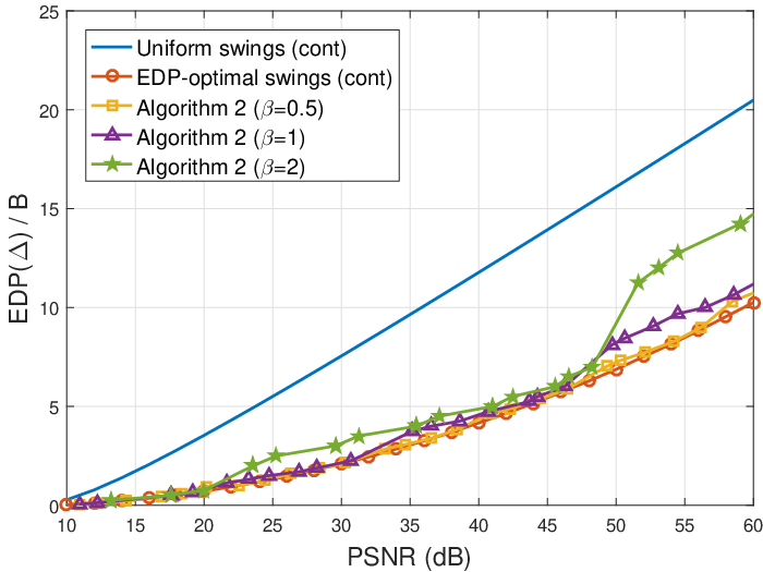
We present an algorithm to obtain discrete swings to minimize EDP in Algorithm 2. The Levin-Campello algorithm cannot solve this problem since the $\rho=\max{(\mathbf{\Delta})}$ in EDP cannot be handled by the Levin-Campello algorithm. By leveraging the sand-pouring and water-filling interpretation of Fig. 5 and KKT conditions, Algorithm 2 attempts to pour sand and fill water iteratively.

Algorithm 2 Sand-pouring and discrete water-filling for (31)

g_{b}\leftarrow\log\frac{\sqrt{2\pi}\sigma}{4^{b}}

for all

b\in[0,B-1]

\triangleright

Set ground level

\mathbf{\Delta}\leftarrow\mathbf{0}

\mathbf{\eta}\leftarrow\mathbf{0}

\mathbf{s}\leftarrow\mathbf{0}

3: while

\mathsf{MSE}(\mathbf{\Delta})>\mathcal{V}

\rho\leftarrow\max(\mathbf{\Delta})

b\leftarrow\underset{b\in[0,B-1]}{\arg\min}~\left\{g_{b}+s_{b}\right\}

\triangleright

Lowest sand level

\eta_{b}\leftarrow\eta_{b}+\beta

\triangleright

Pour more sand

7: for

b=0

B-1

s_{b}\leftarrow\log\left(1+\frac{\eta_{b}}{\rho}\right)

\triangleright

Calculate sand depth

9: end for

10:

b\leftarrow\underset{b\in[0,B-1]}{\arg\min}~\left\{g_{b}+s_{b}+\frac{\Delta_{b}^{2}}{2\sigma^{2}}\right\}

\triangleright

Lowest water level

11:

\Delta_{b}\leftarrow\Delta_{b}+\beta

\triangleright

Fill more water

12: end while

13: return

\mathbf{\Delta}

At each iteration, Algorithm 2 first pours more sand from the lowest sand level as shown in line 5. Note that the sand level of each bit position is the sum of the corresponding ground level and sand depth. We increase $\eta_{b}$ by $\beta$ in line 6 and $\Delta_{b}$ by $\beta$ in line 11 at each iteration to satisfy the optimal condition $\sum{\eta_{b}}=\sum{\Delta_{b}}$ (see (74) in Appendix C). After increasing $\eta_{b}$ , the sand depth $s_{b}$ of each bit position is calculated by Corollary 15, which indicates the increased amount of sand. Afterwards, water is filled from the bit position whose water level is the lowest. Note that the sand depth $s_{b}$ affects the water level unlike Algorithm 1 (Compare line 4 of Algorithm 1 and line 10 of Algorithm 2).

Numerical results in Section VI show that the EDP loss due to discrete swings of Algorithm 2 is negligible for moderate granularity $\beta$ .

VI Numerical Results

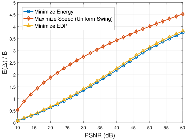
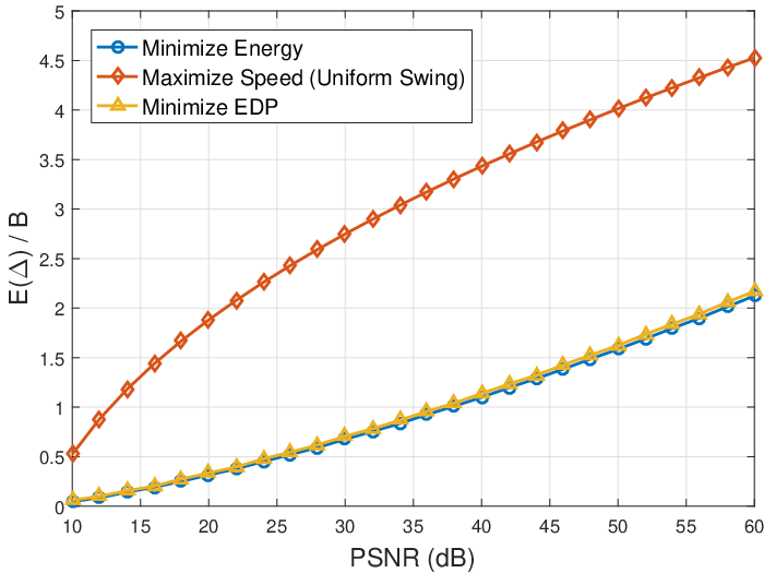
We evaluate the solutions of the three optimization problems for both continuous and discrete swings. Note that the solution of maximizing speed is equivalent to the conventional uniform swing as noted in Remark 11. Also, we compare the proposed optimization solution to LSB dropping and selective ECCs.

Fig. 7 compares the read energy consumption $\mathsf{E}(\mathbf{\Delta})$ as in Definition 1 for a given constraint of peak signal-to-noise ratio (PSNR). The PSNR depends on the MSE as

\mathsf{PSNR}=10\log_{10}{\frac{\left(2^{B}-1\right)^{2}}{\mathsf{MSE}(\mathbf{\Delta})}}.

(53)

At PSNR = 30dB, the optimal solution of (16) (i.e., minimizing energy) reduces the energy consumption by half for $B=8$ , compared to uniform swing (i.e., maximizing speed). For $B=16$ , the energy consumption of energy-optimal swing will be only quarter, compared to the uniform swing. Note that energy consumption of EDP-optimal swing is slightly worse than that of energy-optimal swing.

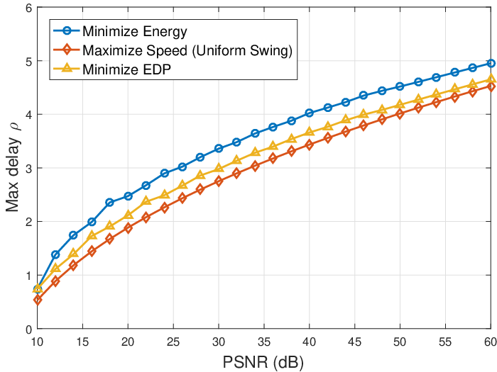
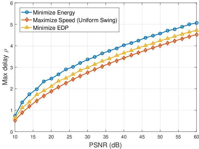
Fig. 8 compares the maximum delay $\rho$ as in Definition 2 for a given PSNR. The conventional uniform swing minimizes the maximum delay; hence it is the speed-optimal solution. The swings minimizing energy achieve significant energy savings at the cost of speed (e.g., the maximum delay increase of 20% at PSNR = 30dB). The EDP-optimal swings increase only 8% of maximum delay at PSNR = 30dB.

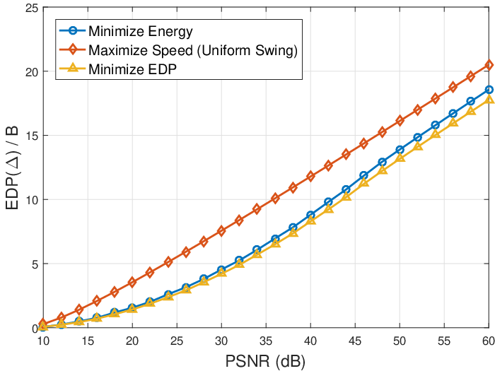
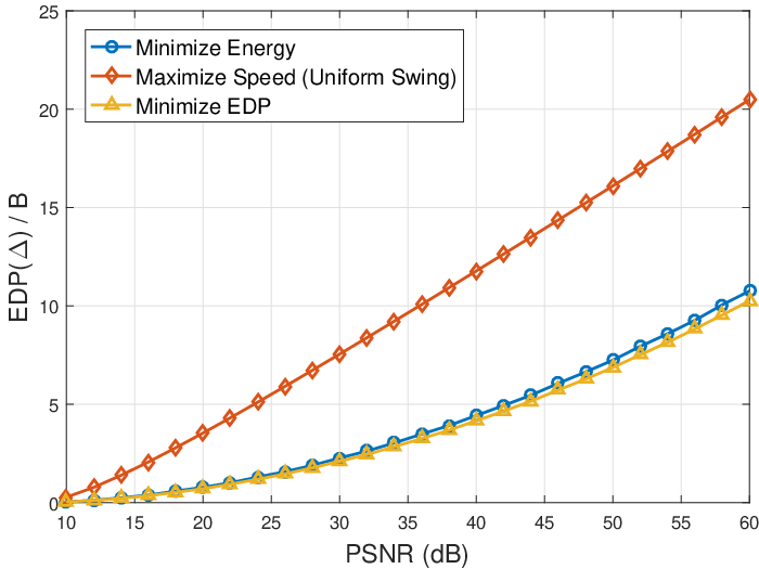
Fig. 9 compares the EDP for a given PSNR. As formulated, the swings minimizing EDP show the best results. The EDP can be reduced by 45% for $B=8$ at PSNR = 30dB. The EDP improvement will be much more for $B=16$ , e.g., 75% EDP saving at PSNR = 30dB. Note that slight loss of speed performance can result in significant energy and EDP savings.

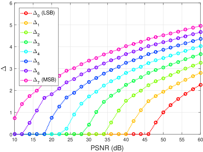
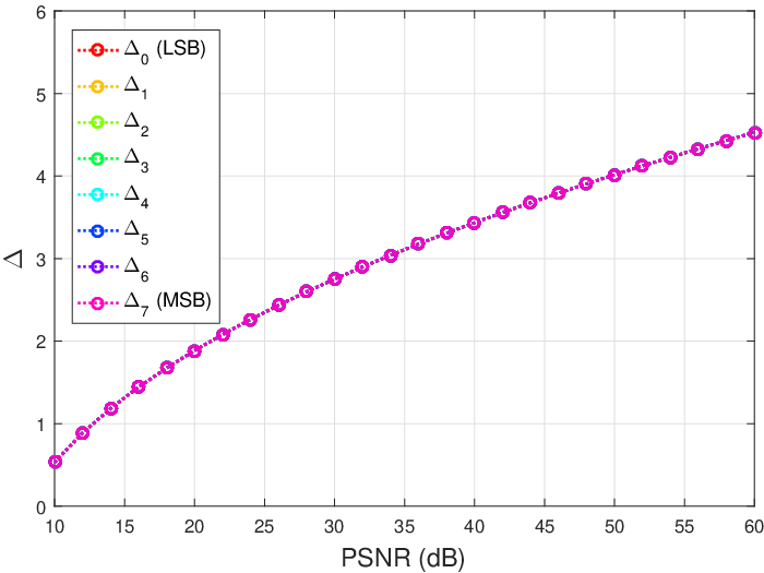
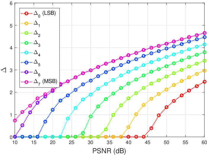
Fig. 10 shows optimal solutions to (a) minimize energy, (b) minimize maximum delay, and (c) minimize EDP. As shown in Fig. 10, we should allocate larger swings for more significant bits. Also, we observe that the swings for several LSBs can be zero depending on PSNR, e.g., $\Delta_{0}=\Delta_{1}=\Delta_{2}=0$ at PSNR = 30dB, a refined kind of LSB dropping. These numerical solutions confirm Theorem 8 and its water-filling interpretation in Fig. 2. Fig. 10 shows the solutions minimizing maximum delay. As we showed in Theorem 10, uniform swings minimize the maximum delay. The optimized swings in Fig. 10 minimize the EDP. Although the EDP-optimal swings are similar to the energy-optimal swings, we observe that $\Delta_{6}=\Delta_{7}=\rho$ at PSNR = 30dB. It is because these two bit positions are filled with sand to suppress the maximum delay as shown in Theorem 14 and its graphical interpretation in Fig. 5.

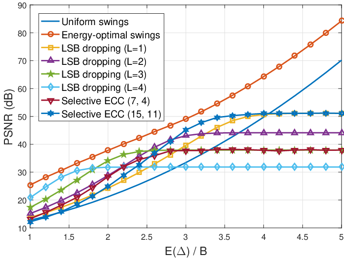
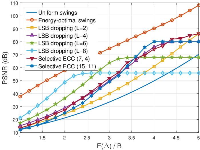
Fig. 11 compares uniform swings, energy-optimal swings (i.e., the optimal solutions of (16)), LSB dropping, and selective ECCs. The proposed energy-optimal swings outperform the other techniques since the energy-optimal swings achieve the target PSNR with the minimum energy $\mathsf{E}(\mathbf{\Delta})$ .

LSB dropping deactivates $L$ LSBs and allocates uniform swings for $(B-L)$ undropped bit positions. In the low PSNR regime, dropping more LSBs (i.e., larger $L$ ) can be effective. However, larger $L$ will limit the levels of achievable PSNRs.

Selective ECCs store parity bits in LSBs to prevent the additional memory overhead. Unlike LSB dropping, selective ECCs allocate uniform swings for all the bit positions. In spite of the LSB information loss, the overall PSNR can be improved by correcting errors in MSBs. As in [18], we consider $(n,k)$ Hamming codes for selective ECCs since complicated ECCs are impractical for SRAMs. In a selective ECC (7, 4) for $B=8$ , the bits of ( $x_{7},x_{6},x_{5},x_{4}$ ) are protected by losing information of $(x_{2},x_{1},x_{0})$ . Since three LSBs are lost, the PSNR of selective ECC (7, 4) converges to the PSNR by LSB dropping $(L=4)$ as shown in Fig. 11. For $B=8$ , a (15, 11) Hamming code cannot be incorporated into an 8-bit word. Hence, we store four parity bits of a Hamming (15, 11) codeword in the last LSBs of four different 8-bit words as proposed in [18]. Note that selective ECC (15, 11) for $B=8$ converges to LSB dropping $(L=1)$ for high $\mathsf{E}(\mathbf{\Delta})$ since both schemes discard only the last LSBs. In Fig. 11, all selective ECCs are applied to one 16-bit word.

Table III compares the PSNRs for uniformly distributed source to real image data (non-uniformly distributed sources) from [39]. Although $p_{0}=\frac{1}{2}$ at PSNR = 20dB (see Fig. 10 and ), we can observe that their PSNRs are almost the same as the PSNRs of uniformly distributed sources as discussed in Section IV-A.

TABLE III: Comparison of PSNRs [dB] of Uniformly Distributed Sources and Real Image Data

PSNR of	PSNR of Airport			PSNR of Fishing Boat			PSNR of Man
uniform source	Min energy	Max speed	Min EDP	Min energy	Max speed	Min EDP	Min energy	Max speed	Min EDP
20	19.99	20.05	20.07	20.19	20.07	20.18	19.75	20.01	19.85
24	24.05	24.01	24.05	24.10	24.06	24.08	23.82	24.00	23.91
28	28.04	28.01	28.03	28.06	28.02	28.09	27.90	28.00	27.95
32	32.00	32.03	32.03	32.04	31.96	32.02	31.95	32.02	31.98
36	36.00	36.00	35.97	36.03	36.05	36.03	35.99	35.97	36.00
40	40.01	39.95	39.95	40.02	40.05	40.07	40.01	40.03	40.03

Fig. 12 shows that the energy penalty due to discrete swings is negligible for moderate granularity $\beta$ . Energy consumption of discrete swings obtained by our Algorithm 1 is almost the same as the Levin–Campello algorithm as explained in Corollary 21.

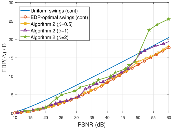
Fig. 13 compares the EDP by optimal swings of Theorem 14 and discrete swings by Algorithm 2. By comparing Fig. 12 to Fig. 13, we observe that the EDP is more sensitive to $\beta$ than the energy. The reason is that the EDP is perturbed by the discretization of $\rho$ as well as the discretization of energy. Nonetheless, the EDP penalty at PSNR = 30dB is very little for moderate granularity such as $\beta=1$ . We can observe that the EDP penalty due to discrete swings is smaller for larger $B$ . Since the Levin–Campello algorithm cannot solve the EDP optimization problem, it is absent in Fig. 13.

VII Conclusion

SRAM is a critical component for information processing systems. Casting read access for SRAMs as an end-to-end communication problem, we found the optimal bit-level swings of SRAMs for applications with fidelity dependent on bit position. We formulated convex optimization problems to determine the optimal swings for the objective functions of energy, maximum delay, and EDP. The optimized bit-level swings can achieve significant energy (50% for 8-bit word and 75% for 16-bit word) and EDP (45% for 8-bit word and 75% for 16-bit word) savings at PSNR of 30dB compared to the conventional uniform swings.

By treating each bit position as an individual channel, we cast bit-level swing optimization problems as generalizations of water-filling that may involve sand-pouring and ground-flattening. Also, we developed optimization algorithms for discrete swings by leveraging water-filling interpretations and KKT conditions. The discrete swings obtained by proposed algorithms achieve almost the same energy and EDP savings as the continuous swings for moderate granularity.

Appendix A Proof of Theorem 8

The KKT conditions of (16) are as follows:

$\displaystyle\sum_{b=0}^{B-1}{4^{b}Q\left(\frac{\Delta_{b}}{\sigma}\right)}\leq\mathcal{V},\quad\nu$	$\displaystyle\geq 0,$	(54)
$\displaystyle\nu\cdot\left\{\sum_{b=0}^{B-1}{4^{b}Q\left(\frac{\Delta_{b}}{\sigma}\right)}-\mathcal{V}\right\}$	$\displaystyle=0,$	(55)
$\displaystyle\Delta_{b}\geq 0,\quad\lambda_{b}\geq 0,\quad\lambda_{b}\Delta_{b}$	$\displaystyle=0$	(56)

for $b\in[0,B-1]$ . From $\frac{\partial L_{1}}{\partial\Delta_{b}}=0$ , $\lambda_{b}$ is given by

\lambda_{b}=1-\nu\cdot\frac{4^{b}}{\sqrt{2\pi}\sigma}\exp{\left(-\frac{\Delta_{b}^{2}}{2\sigma^{2}}\right)}\geq 0.

(57)

By (56) and (57), we obtain

\Delta_{b}\left\{1-\nu\cdot\frac{4^{b}}{\sqrt{2\pi}\sigma}\exp{\left(-\frac{\Delta_{b}^{2}}{2\sigma^{2}}\right)}\right\}=0.

(58)

If $\nu=0$ , then $\lambda_{b}=1$ and $\Delta_{b}=0$ for any $b\in[0,B-1]$ because of (56) and (57). Since $\mathbf{\Delta}=\mathbf{0}$ is a trivial solution, we claim that $\nu\neq 0$ , which results in

\displaystyle\sum_{b=0}^{B-1}{4^{b}Q\left(\frac{\Delta_{b}}{\sigma}\right)}

\displaystyle=\mathcal{V}.

(59)

If $\nu\leq\frac{\sqrt{2\pi}\sigma}{4^{b}}$ , then $\Delta_{b}>0$ is impossible because it would imply $\lambda_{b}=0$ and $\nu=\frac{\sqrt{2\pi}\sigma}{4^{b}}\exp{\left(\frac{\Delta_{b}^{2}}{2\sigma^{2}}\right)}$ , which contradicts the condition $\nu\leq\frac{\sqrt{2\pi}\sigma}{4^{b}}$ . Hence, $\Delta_{b}=0$ for $\nu\leq\frac{\sqrt{2\pi}\sigma}{4^{b}}$ . If $\nu>\frac{\sqrt{2\pi}\sigma}{4^{b}}$ , then $\Delta_{b}=0$ is impossible because it would imply $\nu=\frac{\sqrt{2\pi}\sigma}{4^{b}}\exp{\left(\frac{\Delta_{b}^{2}}{2\sigma^{2}}\right)}=\frac{\sqrt{2\pi}\sigma}{4^{b}}$ , which contradicts the condition $\nu>\frac{\sqrt{2\pi}\sigma}{4^{b}}$ . We claim that $\Delta_{b}>0$ and $\lambda_{b}=0$ , which results in and (19) for $\nu>\frac{\sqrt{2\pi}\sigma}{4^{b}}$ . Thus, the optimal solution $\mathbf{\Delta}^{*}$ of (16) can be derived from (17).

Appendix B Proof of Theorem 10

The KKT conditions of (22) are as follows:

$\displaystyle\sum_{b=0}^{B-1}{4^{b}Q\left(\frac{\Delta_{b}}{\sigma}\right)}\leq\mathcal{V},\quad\nu$	$\displaystyle\geq 0,$	(60)
$\displaystyle\nu\cdot\left\{\sum_{b=0}^{B-1}{4^{b}Q\left(\frac{\Delta_{b}}{\sigma}\right)}-\mathcal{V}\right\}$	$\displaystyle=0,$	(61)
$\displaystyle 0\leq\Delta_{b}\leq\xi,\quad\lambda_{b}\geq 0,\quad\lambda_{b}\Delta_{b}=0,\quad\eta_{b}$	$\displaystyle\geq 0,\quad\eta_{b}(\Delta_{b}-\xi)=0$	(62)

for $b\in[0,B-1]$ . From $\frac{\partial L_{2}}{\partial\Delta_{b}}=0$ and $\frac{\partial L_{2}}{\partial\xi}=0$ , we obtain the following equations:

	$\displaystyle\lambda_{b}=\eta_{b}-\nu\cdot\frac{4^{b}}{\sqrt{2\pi}\sigma}\exp{\left(-\frac{\Delta_{b}^{2}}{2\sigma^{2}}\right)}$	$\displaystyle\geq 0,$		(63)
	$\displaystyle\sum_{b=0}^{B-1}{\eta_{b}}$	$\displaystyle=1$		(64)

From (62) and (63),

\left\{\eta_{b}-\nu\cdot\frac{4^{b}}{\sqrt{2\pi}\sigma}\exp{\left(-\frac{\Delta_{b}^{2}}{2\sigma^{2}}\right)}\right\}\Delta_{b}=0.

(65)

If $\nu=0$ , thIEen $\eta_{b}\Delta_{b}=0$ . Also, note that $\eta_{b}(\Delta_{b}-\xi)=0$ from (62). Both $\eta_{b}\Delta_{b}=0$ and $\eta_{b}(\Delta_{b}-\xi)=0$ result in $\eta_{b}=0$ for any $b\in[0,B-1]$ , which violates (64). Hence, we claim that

\nu>0,\quad\sum_{b=0}^{B-1}{4^{b}Q\left(\frac{\Delta_{b}}{\sigma}\right)}=\mathcal{V}.

(66)

From (63), $\nu\leq\eta_{b}\cdot\frac{\sqrt{2\pi}\sigma}{4^{b}}\exp{\left(\frac{\Delta_{b}^{2}}{2\sigma^{2}}\right)}$ . If $\nu\leq\eta_{b}\cdot\frac{\sqrt{2\pi}\sigma}{4^{b}}$ , then $\Delta_{b}=0$ and $\eta_{b}=0$ , which violates $\nu>0$ of (66). Hence, $\nu>\eta_{b}\cdot\frac{\sqrt{2\pi}\sigma}{4^{b}}$ , which implies $\Delta_{b}>0$ and $\lambda_{b}=0$ for all $b\in[0,B-1]$ because of (62). By $\lambda_{b}=0$ and (63),

\eta_{b}=\nu\cdot\frac{4^{b}}{\sqrt{2\pi}\sigma}\exp{\left(-\frac{\Delta_{b}^{2}}{2\sigma^{2}}\right)}.

(67)

Because of $\nu>0$ and (62), we claim that $\eta_{b}>0$ and

\Delta_{b}=\xi

(68)

for all $b\in[0,B-1]$ . Hence, the optimal solution of (22) is uniform swings, i.e., $\mathbf{\Delta}^{*}=(\xi,\ldots,\xi)$ where $\rho=\max\left(\mathbf{\Delta}^{*}\right)=\xi$ . We confirm that the reformulated problem (22) is equivalent to the original problem (21).

By (67) and (68),

\nu=\frac{\sqrt{2\pi}\sigma}{4^{b}}\cdot\eta_{b}\cdot\exp{\left(\frac{\rho^{2}}{2\sigma^{2}}\right)}

(69)

which is equivalent to (25). From (64) and (69), we obtain (23) and (26).

Appendix C Proof of Theorem 14 and Corollary 15

The KKT conditions of (31) are as follows:

$\displaystyle\sum_{b=0}^{B-1}{4^{b}Q\left(\frac{\Delta_{b}}{\sigma}\right)}\leq\mathcal{V},\quad\nu$	$\displaystyle\geq 0,$	(70)
$\displaystyle\nu\cdot\left\{\sum_{b=0}^{B-1}{4^{b}Q\left(\frac{\Delta_{b}}{\sigma}\right)}-\mathcal{V}\right\}$	$\displaystyle=0,$	(71)
$\displaystyle 0\leq\Delta_{b}\leq\xi,\quad\lambda_{b}\geq 0,\quad\lambda_{b}\Delta_{b}=0,\quad\eta_{b}$	$\displaystyle\geq 0,\quad\eta_{b}(\Delta_{b}-\xi)=0$	(72)

for all $b\in[0,B-1]$ . From $\frac{\partial L_{3}}{\partial\Delta_{b}}=0$ and $\frac{\partial L_{3}}{\partial\xi}=0$ , we obtain the following equations:

	$\displaystyle\xi+\eta_{b}$	$\displaystyle=\lambda_{b}+\nu\cdot\frac{4^{b}}{\sqrt{2\pi}\sigma}\exp{\left(-\frac{\Delta_{b}^{2}}{2\sigma^{2}}\right)},$		(73)
	$\displaystyle\sum_{b=0}^{B-1}{\Delta_{b}}$	$\displaystyle=\sum_{b=0}^{B-1}{\eta_{b}}$		(74)

Suppose that $\nu=0$ , then $\xi+\eta_{b}=\lambda_{b}$ for all $b\in[0,B-1]$ , which implies $\left(\xi+\eta_{b}\right)\Delta_{b}=0$ because of (72). For $b$ such that $\Delta_{b}\neq 0$ , $\eta_{b}=0$ because of $\xi+\eta_{b}=0$ , $\eta_{b}\geq 0$ and $\xi\geq 0$ . For $b$ such that $\Delta_{b}=0$ , $\eta_{b}=0$ because of (72). Hence, if $\nu=0$ , then $\eta_{b}=0$ for all $b\in[0,B-1]$ , which implies $\Delta_{b}=0$ for all $b\in[0,B-1]$ due to $\Delta_{b}\geq 0$ and (74). Thus, we claim that

\nu>0,\quad\sum_{b=0}^{B-1}{4^{b}Q\left(\frac{\Delta_{b}}{\sigma}\right)}=\mathcal{V}

(75)

which is the same as (66).

By (72) and (73),

\lambda_{b}\Delta_{b}=\nu\left\{\frac{\xi+\eta_{b}}{\nu}-\frac{4^{b}}{\sqrt{2\pi}\sigma}\exp{\left(-\frac{\Delta_{b}^{2}}{2\sigma^{2}}\right)}\right\}\Delta_{b}=0

(76)

where $\frac{\nu}{\xi+\eta_{b}}\leq\frac{\sqrt{2\pi}\sigma}{4^{b}}\exp{\left(\frac{\Delta_{b}^{2}}{2\sigma^{2}}\right)}$ because of $\lambda_{b}\geq 0$ . If $\frac{\nu}{\xi+\eta_{b}}\leq\frac{\sqrt{2\pi}\sigma}{4^{b}}$ , then $\Delta_{b}=0$ , which implies $\eta_{b}=0$ by (72). Hence, we claim that

\Delta_{b}=0,\quad\eta_{b}=0,\quad\text{if}~\frac{\nu}{\xi}\leq\frac{\sqrt{2\pi}\sigma}{4^{b}}.

(77)

If $\frac{\nu}{\xi+\eta_{b}}>\frac{\sqrt{2\pi}\sigma}{4^{b}}$ , then $\Delta_{b}>0$ and

\frac{\nu}{\xi+\eta_{b}}=\frac{\sqrt{2\pi}\sigma}{4^{b}}\exp{\left(\frac{\Delta_{b}^{2}}{2\sigma^{2}}\right)}.

(78)

By (72) and (73),

\displaystyle\eta_{b}(\Delta_{b}-\xi)=\nu\left\{\frac{4^{b}}{\sqrt{2\pi}\sigma}\exp{\left(-\frac{\Delta_{b}^{2}}{2\sigma^{2}}\right)}-\frac{\xi-\lambda_{b}}{\nu}\right\}(\Delta_{b}-\xi)=0

(79)

where $\frac{\nu}{\xi-\lambda_{b}}\geq\frac{\sqrt{2\pi}\sigma}{4^{b}}\exp{\left(\frac{\Delta_{b}^{2}}{2\sigma^{2}}\right)}$ because of $\eta_{b}\geq 0$ . If $\frac{\nu}{\xi-\lambda_{b}}\geq\frac{\sqrt{2\pi}\sigma}{4^{b}}\exp{\left(\frac{\xi^{2}}{2\sigma^{2}}\right)}$ , then $\Delta_{b}=\xi>0$ , which implies $\lambda_{b}=0$ by (72). Hence, we claim that

\Delta_{b}=\xi,\quad\lambda_{b}=0,\quad\text{if}~\frac{\nu}{\xi}\geq\frac{\sqrt{2\pi}\sigma}{4^{b}}\exp{\left(\frac{\xi^{2}}{2\sigma^{2}}\right)}.

(80)

If $\frac{\sqrt{2\pi}\sigma}{4^{b}}\leq\frac{\nu}{\xi-\lambda_{b}}<\frac{\sqrt{2\pi}\sigma}{4^{b}}\exp{\left(\frac{\xi^{2}}{2\sigma^{2}}\right)}$ , then

\frac{\nu}{\xi-\lambda_{b}}=\frac{\sqrt{2\pi}\sigma}{4^{b}}\exp{\left(\frac{\Delta_{b}^{2}}{2\sigma^{2}}\right)}.

(81)

By (78) and (81),

\frac{\nu}{\xi+\eta_{b}}=\frac{\nu}{\xi-\lambda_{b}}=\frac{\sqrt{2\pi}\sigma}{4^{b}}\exp{\left(\frac{\Delta_{b}^{2}}{2\sigma^{2}}\right)}

(82)

for $0<\Delta_{b}<\xi$ . $\xi+\eta_{b}=\xi-\lambda_{b}$ (i.e., $\eta_{b}=-\lambda_{b}$ ) means $\eta_{b}=\lambda_{b}=0$ because of $\eta_{b}\geq 0$ and $\lambda_{b}\geq 0$ . Hence, we claim that

\displaystyle\frac{\nu}{\xi}=\frac{\sqrt{2\pi}\sigma}{4^{b}}\exp{\left(\frac{\Delta_{b}^{2}}{2\sigma^{2}}\right)},\quad\eta_{b}=\lambda_{b}=0

(83)

for $\frac{\sqrt{2\pi}\sigma}{4^{b}}<\frac{\nu}{\xi}<\frac{\sqrt{2\pi}\sigma}{4^{b}}\exp{\left(\frac{\xi^{2}}{2\sigma^{2}}\right)}$ .

Due to (74), there should exist $\eta_{b}>0$ for $b\in[0,B-1]$ to make $\sum_{b=0}^{B-1}{\Delta_{b}}>0$ . Hence, there exists $\Delta_{b}=\xi$ due to (72), which implies $\rho=\max(\mathbf{\Delta})=\xi$ . From (77), (80), (83), and $\rho=\xi$ , we can obtain the optimal solution $\mathbf{\Delta}^{*}$ of (32).

Note that $s_{b}>0$ for $\Delta_{b}=\rho$ and $\lambda_{b}=0$ . In this case, (73) can be modified into

\rho+\eta_{b}=\nu\cdot\frac{4^{b}}{\sqrt{2\pi}\sigma}\exp{\left(-\frac{\rho^{2}}{2\sigma^{2}}\right)}.

(84)

As shown in Fig. 5, the sand depth $s_{b}$ is given by

\displaystyle s_{b}

\displaystyle=\log{\frac{\nu}{\rho}}-\left(\log{\frac{\sqrt{2\pi}\sigma}{4^{b}}}+\frac{\rho^{2}}{2\sigma^{2}}\right)=\log{\frac{\nu}{\rho}}-\log{\frac{\nu}{\rho+\eta_{b}}}=\log{\left(1+\frac{\eta_{b}}{\rho}\right)}

(85)

where (85) follows from (84). If $0\leq\Delta_{b}<\rho$ , then $\eta_{b}=0$ as shown in (77) and (83). Hence, $s_{b}=0$ for $0\leq\Delta_{b}<\rho$ . Hence, (35) in Corollary 15 is proved. Also, (37) in Corollary 15 is derived from (74) and (85).

References

[1] M. Horowitz, “Computing’s energy problem (and what we can do about it),” in Proc. IEEE Int. Solid-State Circuits Conf. Dig. Tech. Pap. (ISSCC), Feb. 2014, pp. 10–14.
[2] C.-P. Lin, P.-C. Tseng, Y.-T. Chiu, S.-S. Lin, C.-C. Cheng, H.-C. Fang, W.-M. Chao, and L.-G. Chen, “A 5mW MPEG4 SP encoder with 2D bandwidth-sharing motion estimation for mobile applications,” in Proc. IEEE Int. Solid-State Circuits Conf. Dig. Tech. Pap. (ISSCC), Feb. 2006, pp. 1626–1635.
[3] M. E. Sinangil and A. P. Chandrakasan, “Application-specific SRAM design using output prediction to reduce bit-line switching activity and statistically gated sense amplifiers for up to 1.9 $\times$ lower energy/access,” IEEE J. Solid-State Circuits, vol. 49, no. 1, pp. 107–117, Jan. 2014.
[4] S. Han, X. Liu, H. Mao, J. Pu, A. Pedram, M. A. Horowitz, and W. J. Dally, “EIE: Efficient inference engine on compressed deep neural network,” in Proc. ACM/IEEE 43rd Int. Symp. Comput. Architecture (ISCA), Jun. 2016, pp. 243–254.
[5] Y. H. Chen, T. Krishna, J. S. Emer, and V. Sze, “Eyeriss: An energy-efficient reconfigurable accelerator for deep convolutional neural networks,” IEEE J. Solid-State Circuits, vol. 52, no. 1, pp. 127–138, Jan. 2017.
[6] V. Sze, Y.-H. Chen, T.-J. Yang, and J. Emer, “Efficient processing of deep neural networks: A tutorial and survey,” arXiv preprint arXiv:1703.09039, Mar. 2017. [Online]. Available: http://arxiv.org/abs/1703.09039
[7] B. Zhai, D. Blaauw, D. Sylvester, and S. Hanson, “A Sub-200mV 6T SRAM in 0.13 $\mu m$ CMOS,” in Proc. IEEE Int. Solid-State Circuits Conf. Dig. Tech. Pap. (ISSCC), Feb. 2007, pp. 332–606.
[8] M. H. Abu-Rahma, M. Anis, and S. S. Yoon, “Reducing SRAM power using fine-grained wordline pulsewidth control,” IEEE Trans. VLSI Syst., vol. 18, no. 3, pp. 356–364, Mar. 2010.
[9] I. J. Chang, D. Mohapatra, and K. Roy, “A priority-based 6T/8T hybrid SRAM architecture for aggressive voltage scaling in video applications,” IEEE Trans. Circuits Syst. Video Technol., vol. 21, no. 2, pp. 101–112, Feb. 2011.
[10] J. Kwon, I. J. Chang, I. Lee, H. Park, and J. Park, “Heterogeneous SRAM cell sizing for low-power H.264 applications,” IEEE Trans. Circuits Syst. I, vol. 59, no. 10, pp. 2275–2284, Oct. 2012.
[11] J. George, B. Marr, B. E. S. Akgul, and K. V. Palem, “Probabilistic arithmetic and energy efficient embedded signal processing,” in Proc. Int. Conf. Compilers, Architecture and Synthesis for Embedded Systems (CASES), Oct. 2006, pp. 158–168.
[12] K. Yi, S.-Y. Cheng, F. Kurdahi, and A. Eltawil, “A partial memory protection scheme for higher effective yield of embedded memory for video data,” in Proc. 13th Asia-Pacific Comput. Syst. Architecture Conf., Aug. 2008, pp. 1–6.
[13] M. Cho, J. Schlessman, W. Wolf, and S. Mukhopadhyay, “Reconfigurable SRAM architecture with spatial voltage scaling for low power mobile multimedia applications,” IEEE Trans. VLSI Syst., vol. 19, no. 1, pp. 161–165, Jan. 2011.
[14] X. Yang and K. Mohanram, “Unequal-error-protection codes in SRAMs for mobile multimedia applications,” in Proc. IEEE/ACM Int. Conf. Comput.-Aided Design (ICCAD), Nov. 2011, pp. 21–27.
[15] H. Tang and J. Park, “Unequal-error-protection error correction codes for the embedded memories in digital signal processors,” IEEE Trans. VLSI Syst., vol. 24, no. 6, pp. 2397–2401, Jun. 2016.
[16] H. Kaul, M. Anders, S. Mathew, S. Hsu, A. Agarwal, F. Sheikh, R. Krishnamurthy, and S. Borkar, “A 1.45GHz 52-to-162GFLOPS/W variable-precision floating-point fused multiply-add unit with certainty tracking in 32nm CMOS,” in Proc. IEEE Int. Solid-State Circuits Conf. Dig. Tech. Pap. (ISSCC), Feb. 2012, pp. 182–184.
[17] F. Frustaci, M. Khayatzadeh, D. Blaauw, D. Sylvester, and M. Alioto, “SRAM for error-tolerant applications with dynamic energy-quality management in 28 nm CMOS,” IEEE J. Solid-State Circuits, vol. 50, no. 5, pp. 1310–1323, May 2015.
[18] F. Frustaci, D. Blaauw, D. Sylvester, and M. Alioto, “Approximate SRAMs with dynamic energy-quality management,” IEEE Trans. VLSI Syst., vol. 24, no. 6, pp. 2128–2141, Jun. 2016.
[19] C. H. Huang, Y. Li, and L. Dolecek, “ACOCO: Adaptive coding for approximate computing on faulty memories,” IEEE Trans. Commun., vol. 63, no. 12, pp. 4615–4628, Dec. 2015.
[20] C. E. Shannon, “Communication in the presence of noise,” Proc. IRE, vol. 37, no. 1, pp. 10–21, Jan. 1949.
[21] T. M. Cover and J. A. Thomas, Elements of Information Theory, 2nd ed. Hoboken, NJ: Wiley-Interscience, 2006.
[22] P. S. Chow, “Bandwidth optimized digital transmission techniques for spectrally shaped channels with impulse noise,” Ph.D. dissertation, Stanford University, 1993.
[23] W. Yu and J. M. Cioffi, “On constant power water-filling,” in Proc. IEEE Int. Conf. Commun. (ICC), Jun. 2001, pp. 1665–1669.
[24] A. Lozano, A. M. Tulino, and S. Verdu, “Optimum power allocation for parallel Gaussian channels with arbitrary input distributions,” IEEE Trans. Inf. Theory, vol. 52, no. 7, pp. 3033–3051, Jul. 2006.
[25] A. Macii, L. Benini, and M. Poncino, Memory Design Techniques for Low Energy Embedded Systems. Kluwer Academic Publishers, 2002.
[26] M. H. Abu-Rahma, Y. Chen, W. Sy, W. L. Ong, L. Y. Ting, S. S. Yoon, M. Han, and E. Terzioglu, “Characterization of SRAM sense amplifier input offset for yield prediction in 28nm CMOS,” in Proc. IEEE Custom Integrated Circuits Conf. (CICC), Sep. 2011, pp. 1–4.
[27] M. Horowitz, T. Indermaur, and R. Gonzalez, “Low-power digital design,” in Proc. IEEE Symp. Low Power Electr., Oct. 1994, pp. 8–11.
[28] R. Gonzalez and M. Horowitz, “Energy dissipation in general purpose microprocessors,” IEEE J. Solid-State Circuits, vol. 31, no. 9, pp. 1277–1284, Sep. 1996.
[29] T. Mizuno, J. Okumtura, and A. Toriumi, “Experimental study of threshold voltage fluctuation due to statistical variation of channel dopant number in MOSFET’s,” IEEE Trans. Electron Devices, vol. 41, no. 11, pp. 2216–2221, Nov. 1994.
[30] S. Mukhopadhyay, H. Mahmoodi, and K. Roy, “Modeling of failure probability and statistical design of SRAM array for yield enhancement in nanoscaled CMOS,” IEEE Trans. Comput.-Aided Design Integr. Circuits Syst., vol. 24, no. 12, pp. 1859–1880, Dec. 2005.
[31] M. Abu-Rahma and M. Anis, Nanometer Variation-Tolerant SRAM: Circuits and Statistical Design for Yield. Springer Publishing Company, 2012.
[32] B. S. Leibowitz, J. Kim, J. Ren, and C. J. Madden, “Characterization of random decision errors in clocked comparators,” in Proc. IEEE Custom Integrated Circuits Conf. (CICC), Sep. 2008, pp. 691–694.
[33] D. Knighton, Fluvial Forms and Processes: A New Perspective. London, UK: Arnold, 1998.
[34] J. Maiz, S. Hareland, K. Zhang, and P. Armstrong, “Characterization of multi-bit soft error events in advanced SRAMs,” in IEEE Int. Electron Devices Meeting (IEDM) Tech. Dig., Dec. 2003, pp. 21.4.1–21.4.4.
[35] K. Osada, Y. Saitoh, E. Ibe, and K. Ishibashi, “16.7-fA/cell tunnel-leakage-suppressed 16-Mb SRAM for handling cosmic-ray-induced multierrors,” IEEE J. Solid-State Circuits, vol. 38, no. 11, pp. 1952–1957, Nov. 2003.
[36] B. Fox, “Discrete optimization via marginal analysis,” Manag. Sci., vol. 13, no. 3, pp. 210–216, 1966.
[37] J. Campello, “Optimal discrete bit loading for multicarrier modulation systems,” in Proc. IEEE Int. Symp. Inf. Theory (ISIT), Aug. 1998, p. 193.
[38] ——, “Practical bit loading for DMT,” in Proc. IEEE Int. Conf. Commun. (ICC), Jun. 1999, pp. 801–805.
[39] “USC-SIPI Image Database.” [Online]. Available: http://sipi.usc.edu/database/?volume=misc

Generalized Water-filling for Source-aware Energy-efficient SRAMsThanks: This work was supported in part by Systems on Nanoscale Information fabriCs (SONIC), one of the six SRC STARnet Centers, sponsored by MARCO and DARPA.

Abstract

I Introduction

II SRAM Metrics for Resource and Fidelity

II-A Resource Metrics for Accessing BB-bit Word: Energy, Delay, and EDP

Definition 1

Definition 2

Definition 3

II-B Fidelity Metric for Accessing BB-bit Word: MSE

Remark 4

Definition 5

Lemma 6

Proof:

Lemma 7

Proof:

III Optimal Bit-Level Swings

III-A Energy Minimization

Theorem 8

Proof:

Remark 9 (LSB dropping and constant-power water-filling)

III-B Speed Maximization

Theorem 10

Proof:

Remark 11

Remark 12

Remark 13

III-C EDP Minimization

Theorem 14

Proof:

Corollary 15

Proof:

Remark 16 (Sand-pouring and mercury-filling)

Remark 17 (Ground-flattening and Sand-pouring)

IV Non-uniform Sources and Non-Gaussian Noises

IV-A Non-uniform Sources

Proposition 18

Proof:

Claim 19

Proof:

IV-B Non-Gaussian Noise Models

Claim 20

Proof:

V Architecture and Discrete Swings

V-A Proposed Architecture

V-B Optimization of Discrete Swings: Discrete Water-filling

Corollary 21

Proof:

VI Numerical Results

VII Conclusion

Appendix A Proof of Theorem 8

Appendix B Proof of Theorem 10

Appendix C Proof of Theorem 14 and Corollary 15

References

II-A Resource Metrics for Accessing $B$ -bit Word: Energy, Delay, and EDP

II-B Fidelity Metric for Accessing $B$ -bit Word: MSE