Finite Model Approximations for Partially Observed Markov Decision Processes with Discounted Cost Thanks: This research was supported in part by the Natural Sciences and Engineering Research Council (NSERC) of Canada.
Abstract
We consider finite model approximations of discrete-time partially observed Markov decision processes (POMDPs) under the discounted cost criterion. After converting the original partially observed stochastic control problem to a fully observed one on the belief space, the finite models are obtained through the uniform quantization of the state and action spaces of the belief space Markov decision process (MDP). Under mild assumptions on the components of the original model, it is established that the policies obtained from these finite models are nearly optimal for the belief space MDP, and so, for the original partially observed problem. The assumptions essentially require that the belief space MDP satisfies a mild weak continuity condition. We provide examples and introduce explicit approximation procedures for the quantization of the set of probability measures on the state space of POMDP (i.e., belief space).
I Introduction
In POMDP theory, existence of optimal policies have in general been established via converting the original partially observed stochastic control problem to a fully observed one on the belief space, leading to a belief-MDP. However, computing an optimal policy for this fully observed model, and so for the original POMDP, using well known dynamic programming algorithms is challenging even if the original system has finite state and action spaces, since the state space of the fully observed model is always uncountable. One way to overcome this difficulty is to compute an approximately optimal policy instead of a true optimal policy by constructing a reduced model for the fully observed system for which one can apply well known algorithms such as policy iteration, value iteration, and -learning etc. to obtain the optimal policy.
In MDP theory, various methods have been developed to compute near optimal policies by reducing the original problem into a simpler one. A partial list of these techniques is as follows: approximate dynamic programming, approximate value or policy iteration, simulation-based techniques, neuro-dynamic programming (or reinforcement learning), state aggregation, etc. We refer the reader to [1, 2, 3, 4, 5, 6, 7, 8, 9, 10, 11, 12] and references therein. However, existing works mostly study systems with discrete (i.e., finite or countable) state and action spaces [1, 13, 8, 9, 14, 7]) or those that consider general state and action spaces (see, e.g., [15, 11, 12, 10, 16]) assume in general Lipschitz type continuity conditions on the transition probability and the one-stage cost function in order to provide a rate of convergence analysis for the approximation error. However, for the fully observed reduction of POMDP, a Lipschitz type regularity condition on the transition probability is in general prohibitive. Indeed, demonstrating even the arguably most relaxed regularity condition on the transition probability (i.e., weak continuity in state-action variable), is a challenging problem as was recently demonstrated in [17] for general state and action spaces (see also [18] for a control-free setup). Therefore, results developed in prior literature cannot in general be applied to compute approximately optimal policies for fully observed reduction of POMDP, and so, for the original POMDP.
In [19, 20] we investigated finite action and state approximations of fully observed stochastic control problems with general state and action spaces under the discounted cost and average cost optimality criteria. For the discounted cost case, we showed that optimal policies obtained from these finite models asymptotically achieve the optimal cost for the original problem under the weak continuity assumption on the transition probability. Here, we apply and properly generalize the results in these papers to obtain approximation results for fully observed reduction of POMDPs, and so, for POMDPs. The versatility of approximation results under weak continuity conditions become particularly evident while investigating the applicability of these results to the partially observed case.
In the literature there exist various, mostly numerical and computational, results for obtaining approximately optimal policies for POMDPs. In the following, we list a number of such related results and comparisons with our paper: (i) Reference [21] develops a computational algorithm, utilizing structural convexity properties of the value function of belief-MDPs, for the solutions of POMDPs when the state space is continuous and action and measurements are discrete, and with further extensions to continuous action and measurements. Reference [22] provides an algorithm which may be regarded as a quantization of the belief space. However, no rigorous convergence results are given regarding this computational algorithm. (ii) References [23] and [24] present quantization based algorithms for the belief state, where the state, measurement, and the action sets are finite. (iii) References [25] and [26] provide an explicit quantization method for the set of probability measures containing the belief states, where the state space, unlike in many other contributions in the literature, is continuous. The quantization is done through the approximations as measured by Kullback-Leibler divergence: Kullback-Leibler divergence (or relative entropy) is a very strong pseudo-distance measure which is even stronger than total variation (by Pinsker’s inequality [27]), which in turn is stronger than weak convergence. In particular, being able to quantize the space of probability measures with finitely many balls as defined by such a distance measure requires very strict assumptions on the allowable beliefs and it in particular requires, typically equicontinuity conditions (see e.g. [28, Lemma 4.3]). (iv) In [29] the authors consider the near optimality of finite-state controllers that are finite-state probabilistic automatons taking observations as inputs and producing controls as the outputs. A special case for these type of controllers are the ones that only use finite observation history. A similar finite memory approximation is developed in [30]. (v) In [31] the authors establish finite state approximation schemes for the belief-MDPs under both discounted cost and average cost criteria using concavity properties of the corresponding value function and show that approximate costs can be used as lower bounds for the optimal cost function. A similar finite state approximation is considered in [32, 33] using concavity and convexity properties of the value function for the discounted cost criterion. We refer the reader to the survey papers [34, 35] and the book [36] for further algorithmic and computational procedures for approximating POMDPs.
Contributions of the paper. (i) We show that finite models asymptotically approximate the original partially observed Markov decision process (POMDP) in the sense that the true costs of the policies obtained from these finite models converge to the optimal cost of the original model. The finite models are constructed by discretizing both the state and action spaces of the equivalent fully-observed belief space formulation of the POMDP. We establish the result for models with general state and action spaces under mild conditions on the system components. (ii) We provide systematic procedures for the quantization of the set of probability measures on the state space of POMDPs which is the state space of belief-MDPs. (iii) Our rigorous results can be used to justify the novel quantization techniques presented in [22, 23, 24] as well as a more relaxed version for the results presented in [25] and [26]. In particular, there do not exist approximation results of the generality presented in our paper with asymptotic performance guarantees. We show that provided that the belief space is quantized according to balls generated through metrics that metrize the weak convergence topology (such as Prokhorov, bounded-Lipschitz, or stronger ones such as the Wasserstein metric), and provided that the action sets are quantized in a uniform fashion, under very weak conditions on the controlled Markov chain (namely the weak continuity of the kernel and total variation continuity of the measurement channel), asymptotic optimality is guaranteed. (iv) Our approach also highlights the difficulties of obtaining explicit rates of convergence results for approximation methods for POMDPs. Even in fully observed models, for obtaining explicit rates of convergence, one needs strong continuity conditions of the Lipschitz type, e.g.; [20, Theorem 5.1]. As Theorem 1 shows, this is impossible under even quite strong conditions for POMDPs.
The rest of the paper is organized as follows. In Section II we introduce the partially observed stochastic control model and construct the belief space formulation. In Section III we establish the continuity properties that are satisfied by the transition probability of the belief space MDP and state approximation results. In Section VI we illustrate our results by considering numerical examples. Section VII concludes the paper.
II Partially Observed Markov Decision Processes
A discrete-time partially observed Markov decision process (POMDP) has the following components: (i) State space , action space , and observation space , all Borel spaces, (ii) is the transition probability of the next state given the current state-action pair is , (iii) is the observation channel giving the probability of the current observation given the current state variable , and (iv) the one-stage cost function .
The key difference of POMDPs from the fully observed MDP is that the state of the system cannot be observed directly by the controller. Instead, the noisy version of the state is available to the controller through an observation channel or . These type of problems in general arise when there is an uncertainty in measurements of the states or there are some states which cannot be measured.
To complete the description of the partially observed control model, we must specify how the controller designs its control law at each time step. To this end, define the history spaces and , endowed with their product Borel -algebras generated by and . A policy is a sequence of stochastic kernels on given . We denote by the set of all policies.
According to the Ionescu Tulcea theorem [37], an initial distribution on and a policy define a unique probability measure on . The expectation with respect to is denoted by . For any initial distribution and policy we can think of the POMDP as a stochastic process defined on the probability space , where , the are -valued random variables, the are -valued random variables, the are -valued random variables, and they satisfy for all
where , , and . We denote by the discounted cost function of the policy with initial distribution , which is given by
where is the discount factor.
With this notation, the discounted value function of the control problem is defined as
A policy is said to be optimal if .
In POMDPs, since the information available to the decision maker is a noisy version of the state, one cannot apply the dynamic programming principle directly as the one-stage cost function depends on the exact state information. A canonical way to overcome this difficulty is converting the original partially observed control problem to a fully observed one on the belief space. Indeed, let us define
Here, is the posterior state distributions or ’beliefs‘ of the observer at time in the original problem. One can prove that, for any , we have
where is a fixed stochastic kernel on given (see next section for the construction of ). Note that . Furthermore, define the one-stage cost function as
Hence, we obtain a fully-observed Markov decision process with the components . This MDP is called the belief-MDP and it is equivalent to the original POMDP in the sense that for any optimal policy for the belief-MDP, one can construct a policy for the original POMDP which is optimal. The following observations are crucial in obtaining the equivalence of these two models: (i) any history vector of the belief-MDP is a function of the history vector of the original POMDP and (ii) history vectors of the belief-MDP is a sufficient statistic for the original POMDP.
Therefore, results developed for MDPs can be applied to the belief-MDP and so, to the POMDP. However, one should keep in mind that the correspondence between policies of the belief-MDP and the POMDP is quite complicated as one has to compute the so-called non-linear filtering equation [38] at each time step. Moreover, stationary policies in the belief-MDP can be history dependent in the original POMDP. Therefore, establishing structural properties of optimal policies for the belief-MDP in general does not give much information about the optimal policies for the original POMDP. However, we will see in the sequel that the belief-MDP formulation of the POMDP is useful in the finite-model approximation problem.
III Continuity Properties of Belief-MDPs
In this section, we first discuss the continuity properties that are satisfied by or prohibitive for the transition probability of the belief-MDP. Then, we derive the conditions satisfied by the components of the belief-MDP.
III-A On the Convergence of Probability Measures
Let be a Borel space and let denote the family of all probability measure on . A sequence is said to converge to weakly (resp., setwise) if
for all continuous and bounded real function (resp., for all measurable and bounded real function ).
For any , the total variation norm is given by
where the supremum is over all measurable real such that . A sequence is said to converge to in total variation if . As it is clear from the definitions, total variation convergence implies setwise convergence, which in turn implies weak convergence.
The total variation metric leads to a stringent notion for convergence. For example a sequence of discrete probability measures on a finite-dimensional Euclidean space never converges in total variation to a probability measure which admits a density function with respect to the Lebesgue measure. Setwise convergence also induces a topology which is not easy to work with since the space under this convergence is not metrizable [39, p. 59]. However, the space of probability measures on a Borel space endowed with the topology of weak convergence is itself a Borel space [40]. The bounded-Lipschitz metric [41, p.109], for example, can be used to metrize this space:
| (1) |
where
and is the metric on . Finally, the Wasserstein metric of order 1, , can also be used for compact (see [41, Theorem 6.9]):
where denotes the set of probability measures on with first marginal and second marginal . Indeed, can also be used as an upper bound to for non-compact since can equivalently be written as [41, Remark 6.5]:
where
Comparing this with (1), it follows that
| (2) |
This observation will be utilized for the quantization algorithms on the set of probability measures later in the paper.
III-B Continuity Properties under a Belief Space Formulation of POMDPs
As indicated in Section II, any POMDP can be reduced to a (completely observable) MDP [42], [43], whose states are the posterior state distributions or beliefs of the observer; that is, the state at time is
In this section, we construct the components of this belief-MDP (in particular transition probability ) under some assumptions on the components of the POMDP. Later, we establish the conditions satisfied by the components of the belief-MDP, under which we can apply approximation results in our earlier work [19, 20] to the belief-MDP, and so, to the original POMDP.
To this end, let be a continuous moment function in the sense that there exists an increasing sequence of compact subsets of such that
The following assumptions will be imposed on the components of the POMDP.
Assumption 1.
The one-stage cost function is continuous and bounded.
The stochastic kernel is weakly continuous in , i.e., if , then weakly.
The observation channel is continuous in total variation, i.e., if , then in total variation.
is compact.
There exists a constant such that
The initial probability measure satisfies
We let
Note that since the probability law of is in , by Assumption 1-(e),(f), under any policy we have almost everywhere. Therefore, the belief-MDP has state space instead of , where is equipped with the Borel -algebra generated by the topology of weak convergence. The transition probability of the belief-MDP can be constructed as follows (see also [38]). Let denote the generic state variable for the belief-MDP. First consider the transition probability on given
where . Let us disintegrate as
Then, we define the mapping as
| (3) |
In the literature, (3) is called the ‘nonlinear filtering equation’ [38]. Note that, for each , we indeed have
| and | ||||
Then, can be written as
where denotes the Dirac-delta measure at point ; that is, if and otherwise it is zero. Recall that the initial point for the belief-MDP is ; that is, , and the one-stage cost function of the belief-MDP is given by
| (4) |
Hence, the belief-MDP is a fully-observed Markov decision process with the components
For the belief-MDP define the history spaces and , and let denote the set of all policies for the belief-MDP, where the policies are defined in a usual manner. Let denote the discounted cost function of policy for initial distribution of the belief-MDP.
Notice that any history vector of the belief-MDP is a function of the history vector of the POMDP. Let us write this relation as . Hence, for a policy , we can define a policy as
| (5) |
Let us write this as a mapping from to : . It is straightforward to show that the cost functions and are the same, where . One can also prove that (see [42], [43])
| (6) |
and furthermore, that if is an optimal policy for the belief-MDP, then is optimal for the POMDP as well. Hence, the POMDP and the corresponding belief-MDP are equivalent in the sense of cost minimization. Therefore, approximation results developed for MDPs in [19, 20] can be applied to the belief-MDP and so, to the POMDP.
III-C Strong and Weak Continuity Properties of the Belief MDP
The stochastic kernel is said to be weakly continuous if weakly, whenever . The kernel is said to be strongly continuous if, for any , setwise, whevener . For the fully observed reduction of a partially observed MDP (POMDP), requiring strong continuity of the transition probability is in general too strong condition. This is illustrated through the following simple example.
Example 1.
Consider the system dynamics
where , , , and where , , and are the state, observation and action spaces, respectively, all of which we take to be (the nonnegative real line) and the ‘noise’ process is a sequence of i.i.d. random variables uniformly distributed on . It is easy to see that the transition probability is weakly continuous with respect to state-action variables and the observation channel is continuous in total variation with respect to state variable for this POMDP. Hence, by [44, Theorem 3.7] the transition probability of the belief-MDP is weakly continuous in the state-action variables. However, the same conclusion cannot be drawn for the setwise continuity of with respect to the action variable as shown below.
Recall that is given by
where , , and is the posterior distribution of the state given the past observations, i.e.,
Let us set (point mass at ), , and . Then , but as we next show, does not converge to setwise.
Observe that for all and , we have and . Define the open set with respect to the weak topology in as
where if and otherwise. Observe that we have for all and , but for all . Hence,
| but | ||||
implying that does not converge to setwise. Hence, does not satisfy the strong continuity assumption.
The following theorem is a consequence of [44, Theorem 3.7, Example 4.1] and the preceding example.
Theorem 1.
Under Assumption 1-(b),(c), the stochastic kernel for belief-MDP is weakly continuous in .
If we relax the continuity in total variation of the observation channel to setwise or weak continuity, then may not be weakly continuous even if the transition probability of POMDP is continuous in total variation.
Finally, may not be setwise continuous in action variable even if the observation channel is continuous in total variation.
Part (i) of Theorem 1 implies that the transition probability of the belief-MDP is weakly continuous under Assumption 1. However, note that continuity of the observation channel in total variation in Assumption 1 cannot be relaxed to weak or setwise continuity. On the other hand, the continuity of the observation channel in total variation is not enough for the setwise continuity of .
The above suggest that our earlier results in [19] and [20], which only require weak continuity conditions on the transition kernel of a given MDP, are particularly suitable in developing approximation methods for POMDPs (through their MDP reduction), in both quantizing the action spaces as well as state spaces.
Remark 1.
We refer the reader to [44, Theorem 3.2(c)] for more general conditions implying weak continuity of the transition probability . We also note that, in the uncontrolled setting, [45] and [18] have established similar weak continuity conditions (i.e., the weak-Feller property) of the non-linear filter process (i.e., the belief process) in continuous time and discrete time, respectively.
Example 2.
In this example we consider the following partially observed model
| (7) |
where , , and for some . The noise processes and are sequences of independent and identically distributed (i.i.d.) random vectors taking values in and , respectively, for some , and they are also independent of each other. In this system, the continuity of in is sufficient to imply the weak continuity of the transition probability , and no assumptions are needed on the noise process (not even the existence of a density is required). On the other hand, the continuity of the observation channel in total variation holds, if for any , the probability measure has a density , which is continuous in , with respect to some reference probability measure on . This follows from Scheffé’s theorem (see, e.g., [46, Theorem 16.2]). For instance, this density condition holds for the following type of models:
- (i)
In the first model, we have , , is continuous, and has a continuous density with respect to Lebesgue measure.
- (ii)
In the second case, is countable and is continuous in for all . Therefore, the transition probability of the belief space MDP, corresponding to the model in (7), is weakly continuous.
Next, we derive conditions satisfied by the components of the belief-MDP under Assumption 1. Note first that , where
Since is a moment function, each is tight [37, Proposition E.8]. Moreover, each is also closed since is continuous. Therefore, each is compact with respect to the weak topology. This implies that is a -compact Borel space. Note that by [47, Proposition 7.30], the one-stage cost function of the belief-MDP, which is defined in (4), is in under Assumption 1-(a). Therefore, the belief-MDP satisfies the following conditions under Assumption 1, which we formally state as a separate assumption.
Assumption 2.
The one-stage cost function is bounded and continuous.
The stochastic kernel is weakly continuous.
is compact and is -compact.
IV Finite Model Approximations
IV-A Finite-Action Approximation
In this section, we consider finite-action approximation of the belief-MDP and so, the POMDP. For these equivalent models, we obtain an approximate finite-action model as follows. Let denote the metric on . Since is assumed compact and thus totally bounded, there exists a sequence of finite sets such that for each ,
In other words, is a -net in . The sequence is used by the finite-action model to approximate the belief-MDP and the POMDP.
In [19], for MDPs with Borel state and action spaces, we studied the problem of approximating an uncountable action set with a finite one and had established the asymptotic optimality of finite action models for such fully observed MDPs that satisfy a number of technical conditions, in particular, the weak continuity condition of the transition kernel in state and action variables. Given the belief-MDP reduction, [19, Theorem 3.2] implies the following result.
Theorem 2.
The significance of Theorem 2 is reinforced by the following observation. If we let to be the set of deterministic policies of the POMDP taking values in , then the theorem implies that for any given there exists and such that
where (see (5)) and is the optimal deterministic stationary policy for the belief-MDPn.
IV-B Finite-State Approximation
The finite-state model for the belief-MDP is obtained as in [20], by quantizing the set of probability measures ; that is, for each , we quantize compact set similar to the quantization of and represent the rest of the points by some pseudo-state.
If is compact, in the following, the index can be fixed to .
We let denote a metric on which metrizes the weak topology. For each , since is compact and thus totally bounded, there exists a sequence of finite grids in such that for all ,
| (8) |
Let be a partition of such that and
| (9) |
for all . Choose any which is a so-called pseudo-state and set . Let and define function by
Here maps to the representative element of the partition it belongs to.
Remark 2.
- (a)
Note that given that satisfies (8), one way to obtain the corresponding partition of satisfying (9) as follows. Let us define function as
where ties are broken so that is measurable. In the literature, is often called a nearest neighbor quantizer with respect to ’distortion measure‘ [48]. Then, induces a partition of the space given by
and which satisfies (9). Although one can construct, in theory, the partition using nearest neighbor sense, it is computationally difficult to find these regions when the original state space is uncountable.
- (b)
The index indicates the resolution of the quantizer that is applied to discretize the compact set and index emphasizes the size of the compact set for which quantization is applied.
Let be a sequence of probability measures on satisfying
| (10) |
One possible choice for is
We let be the restriction of to defined by
The measures will be used to define a sequence of finite-state belief MDPs, denoted as MDP, which approximate the belief-MDP. To this end, for each and define the one-stage cost function and the transition probability on given by
| (11) |
where is the pushforward of the measure with respect to ; that is,
for all . For each and , we define MDP as a Markov decision process with the following components: is the state space, is the action space, is the transition probability, and is the one-stage cost function.
Given the belief-MDP, [20, Theorem 3.2]11 1 Although Theorem 3.2 in [20] is proved under the assumption that the state space is locally compact, a careful examination of the proof reveals that -compactness of the state space is also sufficient to establish the result. implies the following.
Theorem 3.
Theorem 3 implies that to find a near optimal policy for the POMDP, it is sufficient to compute an optimal policy for the finite-state belief-MDP with sufficiently many states, extend this policy to the original state space of the belief-MDP, and then construct the corresponding policy for the POMDP.
In the following, we discuss explicit methods to quantize the set of probability measures on , that is, the belief-space .
V Quantization of the Belief-Space
An explicit construction for an application requires a properly defined metric on . As stated in Section III-A, one can metrize the set of probability measures defined on a Borel space under the weak topology using various distance measures. Building on this fact, in the following we present explicit methods for the quantization of for the cases where is finite, a compact subset of a finite dimensional Euclidean space, or the finite-dimensional Euclidean space itself, and is independent of the state variable .
V-A Construction with Finite
If the state space is finite with , then , and is a simplex in . In this case, Euclidean distance can be used to metrize . Indeed, one can make use of the algorithm in [49] (see also [50]) to quantize in a nearest neighbor manner. To this end, for each , define
| (12) |
where is the set of rational numbers and . The set is called type lattice by analogy with the concept of types in information theory [51, Chp. 12]. Then, the algorithm that computes the nearest neighbor levels can be described as follows:
Algorithm. Given , find nearest
- (1)
Compute values ()
- (2)
If the nearest is given by . Otherwise, compute the errors
and sort them - (3)
Let . If , set
If , set
Then, the nearest is given by .
One can also compute the maximum radius of the quantization regions for this algorithm. To this end, let and denote respectively the metrics induced by and () norms on , which metrizes the weak topology on . Then, we have [49, Proposition 2]
where . Hence, for each , the set is an -net in with respect to metric, where .
V-B Construction with Compact
The analysis in the previous subsection shows that a finitely supported measure can be approximated through type lattices. Thus, if compactly supported probability measures can be approximated with those having finite support, the analysis in Section V-A yields approximately optimal policies. In the following, we assume that is a compact subset of for some . Then is also compact (under the weak convergence topology) and can be metrized using the Wasserstein metric (here, in defining , we use the metric on induced by the Euclidean norm ) as discussed in Section III-A.
For each , let be some lattice quantizer [48] on such that for all . Set , i.e., the output levels of (note that is finite since is compact). Then, one can approximate any probability measure in with probability measures in
Indeed, for any , we have [52, Theorem 2.6]
Once this is obtained, we can further approximate the probability measure induced by via the algorithm introduced in Section V-A with asymptotic performance guarantees. Thus, through a sequence of type lattices as given in (12) with a successively refined support set so that for with , one can quantize to obtain a sequence of finite state-action MDPs through (11) leading to Theorem 3.
For some related properties of approximations of probability measures with those with finite support, and the relation to optimal quantization, we refer the reader to [52].
V-C Construction with Non-compact
Here we assume that for some and that Assumption 1 holds for . In this case, becomes the set of probability measures with finite second moment and is the set of probability measures with finite second moments bounded by . We endow here with the bounded-Lipschitz metric , which metrizes weak convergence (see Section III-A).
We first describe the discretization procedure for . For each , set and let denote a lattice quantizer on satisfying
Let denote the set of output levels of ; that is, . Define
Let . Then, any measure in can be approximated by probability measures in
Indeed, for any , we have
| (13) | ||||
| (14) |
In the derivation above, (13) follows from (2). Thus, in can be approximated by the , which is induced by the quantizer , with a bound . Then, similar to Section V-B, we can further approximate probability measure via the algorithm introduced in Section V-A with again asymptotic performance guarantees by Theorem 3. Thus, analogous to compact case, using a sequence of type lattices as given in (12) with a successively refined support set for with , one can quantize to obtain a sequence of finite state-action MDPs through (11).
V-D Construction for Special Models leading to Quantized Beliefs with Continuous Support
So far, we have obtained quantized beliefs where each such quantized belief measure was supported on a finite set. For some applications, this may not be efficient and it may be more desirable to quantize the measurement space appropriately. For some further applications, a parametric representation of the set of allowable beliefs may be present and the construction of bins may be more immediate through quantizing the parameters in a parametric class. What is essential in such models is that the bins designed to construct the finite belief-MDP correspond to balls which are small under the metrics that metrize the weak convergence as discussed in Section III-A.
V-D1 Quantized Measures Through Quantized Measurements
For this section, we assume that transition probability is independent of the state variable , for some , and Assumption 1 holds for some . In the view of Theorem 2, as a pre-processing set-up, we quantize the action space , where the finite set represents the output levels of this quantizer. Hence, in the sequel, we assume that the action space is .
Since , we have
and so, the disintegration of becomes
Then, is given by
This implies that we can take the following set as the state space of the fully-observed model instead of :
We endow with the bounded-Lipschitz metric . For each , set and let denote a lattice quantizer on satisfying
Let denote the set of output levels of ; that is, . Define
Then, finite set , which is used to quantize , is given by
and the corresponding quantizer is defined as follows: given , we define
Note that to use for constructing finite models, we have to obtain an upper bound on the -distance between and . This can be achieved under various assumptions on the system components. One such assumption is the following: (i) for some , (ii) is compact, (ii) and , (iv) is Lipschitz continuous with Lipschitz constant , for some , and . Since is compact, there exists for each such that as and for all . Under the above assumptions, we have
where
Since the bounded-Lipschitz metric is upper bounded by the total variation distance, we obtain
Hence, is a legitimate quantizer for constructing the finite models. Section VI-B exhibits another example where we have such an upper bound.
V-D2 Construction from a Parametrically Represented Class
For some applications, the set of belief measures can be first approximated by some parametric class of measures, where parameters belong to some low-dimensional space [53, 26, 54]. For instance, in [26], densities of belief measures are projected onto exponential family of densities using the Kullback-Leibler (KL) divergence, where it was assumed that projected beliefs are close enough to true beliefs in terms of cost functions. In [54], densities are parameterized by unimodal Gaussian distributions and parameterized MDP are solved through Monte Carlo simulation based method. In [53], densities are represented by sufficient statistics, and in particular represented by Gaussian distributions, and the parameterized MDP is solved through fitted value iteration algorithm. However, among these works, only the [26] develop rigorous error bounds for their algorithms using the KL divergence and the other works do not specify distance measures to quantify parametric representation approximations.
In these methods, if the parameterized beliefs are good enough to represent true beliefs as it was shown in [26], then the method presented in the earlier sections (of first quantizing the state space, and then quantizing the beliefs on the state space) may not be necessary and one can, by quantizing the parameters for the class of beliefs considered, directly construct the finite belief-MDP. As noted earlier, what is essential in such methods is that the bins designed to construct the finite belief-MDP correspond to balls which are small under the metrics that metrize the weak convergence as discussed in Section III-A. This possible if the projected beliefs are proved to be close to the true beliefs with respect to some metric that generates the weak topology or with respect to some (pseudo) distance which is stronger than weak topology. For instance, since convergence in KL-divergence is stronger than weak convergence, the projected beliefs constructed in [26] indeed satisfies this requirement. Hence, one can apply our results to conclude the convergence of the reduced model to the original model in [26]. As noted earlier, relative entropy is a very strong pseudo-distance measure which is even stronger than total variation (by Pinsker’s inequality [27]) and for being able to quantize a set of probability measures with finitely many balls as defined by such a distance measure requires very strict assumptions on the allowable beliefs and it in particular requires, typically equicontinuity conditions (see e.g. [28, Lemma 4.3]). In turn, it is in general necessary to assume that transition probability and observation channel have very strong regularity conditions.
VI Numerical Examples
In this section, we consider two examples in order to illustrate our results numerically. Since computing true costs of the policies obtained from the finite models is intractable, we only compute the value functions of the finite models and illustrate their converge as . We note that all results in this paper apply with straightforward modifications for the case of maximizing reward instead of minimizing cost.
VI-A Example with Finite
We consider a machine repair problem in order to illustrate our results numerically for finite state POMDPs. In this model, we have with the following interpretation:
| and | ||||
There are two sources of uncertainty in the model. The first one is the measurement uncertainty. The probability that the measured state is not the true state is given by ; that is,
In other words, there is a binary symmetric channel with crossover probability between the state process and the observation process.
The second uncertainty comes from the repair process. In this case, is the probability that the machine repair was successful given an initial ‘not working’ state:
Finally, the probability that the machine does not break down in one time step is denoted by :
The one-stage cost function for this model is given by:
where is defined to be the cost of repair and is the cost incurred by a broken machine. The cost function to be minimized is the discounted cost function with a discount factor .
In order to find the approximately optimal policies, we first construct the belief space formulation of the above model. Note that the state space of the belief space model is the interval . Hence, we can use uniform quantization on to obtain the finite model.
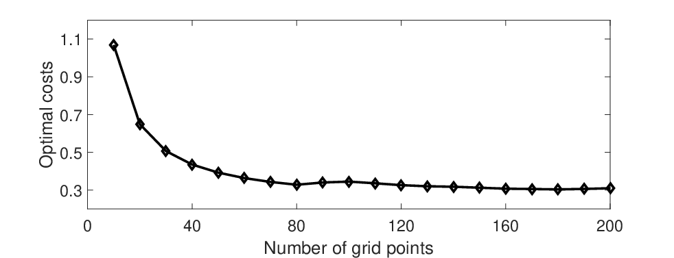
For the numerical results, we use the following parameters: , , , and . We selected 20 different values for the number of grid points to discretize : . The grid points are chosen uniformly. For each , the finite state models are constructed as in [20, Section 2].
Figure 1 shows the graph of the value functions of the finite models corresponding to the different values of (number of grid points), when the initial state is . It can be seen that the value functions converge (to the value function of the original model by [20, Theorem 2.4]).
VI-B Example with Compact
In this example we consider the following model:
| (15) | ||||
| (16) |
where , is the state at , and is the action at . The one-stage ‘reward’ function is , where is some utility function. In this model, the goal is to maximize the discounted reward. This model is the modified and partially observed version of the population growth model in [37, Section 1.3].
The state and action spaces are , for some , and the observation space is for some . Since is merely a constant, by taking as our new action space, instead of dynamics in equation (15) we can write the dynamics of the state as
The noise processes and are sequences of independent and identically distributed (i.i.d.) random variables which have common densities supported on and supported on , respectively. Therefore, the transition probability is given by
for all and the observation kernel is given by
for all . To make the model consistent, we must have for all . We assume that and are uniform probability density functions; that is, on and on . Hence, Assumption 1 holds for this model with .
In the view of Theorem 2, as a pre-processing set-up, we quantize the action space , where the finite set represents the output levels of this quantizer with . In the remainder of this example we assume that the action space is .
We now obtain the stochastic kernels and that describe the transition probability of the reduced MDP. Indeed, we have
where is given by
Similarly, we have
where is given by
| (17) |
Hence, for any , the transition probability has a support on the set of probability measures on having densities given by (17). This implies that we can take the following set as the state space of the fully-observed model instead of :
Note that for some , probability density function is not well-defined as , and so, we disregard these points. For the rest of the points in , a typical can be in the following forms:
| (18) | ||||
| (19) | ||||
| (20) |
For each , let denote the uniform quantizer on having output levels; that is,
| where , , and | ||||
where . We define
Then, the quantizer , which is used to construct the finite model, is defined as follows: given , we define
To be able to use for constructing finite models, we need to obtain an upper bound on the -distance between and . To this end, let be a small constant such that .
Suppose that the density of is in the form of (19); that is, and for some . Let , , and . Since is a continuous function of and is compact, there exists which is independent of such that and as . We also suppose that without loss of generality. Then, for sufficiently large , by using the inequality , we obtain
where
Hence, as . Similar computations can be done for of the form (18) and (20). This implies that is a legitimate quantizer to construct finite-state models.
For the numerical results, we use the following values of the parameters:
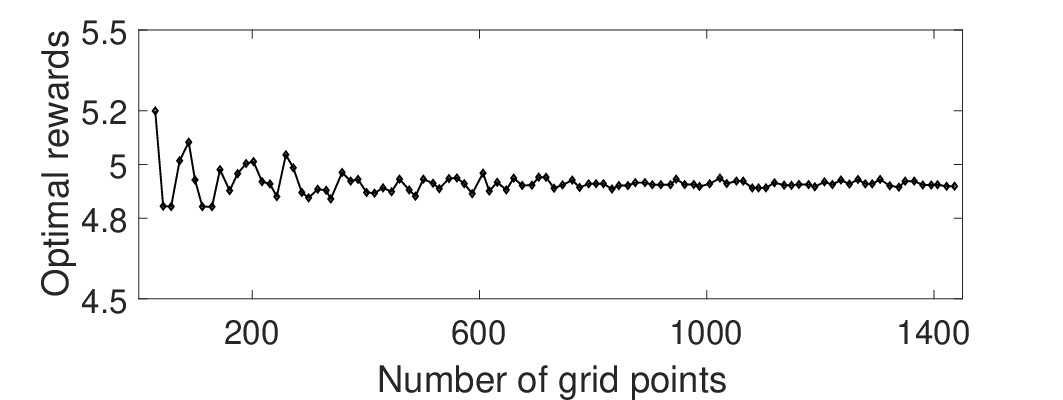
The utility function is taken to be quadratic function; i.e., . As a pre-processing set-up, we first uniformly discretize the action space by using the 20 grid points. Then, we selected 99 different values for the number of grid points to discretize the state space using the quantizer , where varies from to .
We use the value iteration algorithm to compute the value functions of the finite models. The simulation was implemented by using MATLAB and it took 411.75 seconds using an HP EliteDesk 800 desktop computer. Figure 2 displays the graph of these value functions corresponding to the different values for the number of grid points, when the initial state is . The figure illustrates that the value functions of the finite models converge (to the value function of the original model by [20, Theorem 2.4]).
VII Concluding Remarks
We studied the approximation of discrete-time partially observed Markov decision processes under the discounted cost criterion. An essential observation was that establishing strong continuity properties for the reduced (belief) model is quite difficult for general state and action models, whereas weak continuity can be established under fairly mild conditions on the transition kernel of the original model and the measurement equations. This allowed us to apply our prior approximation results [19, 20], developed under weak continuity conditions, to partially observed models.
In particular, [19, 20] developed finite model approximation for both the discounted and the average cost criteria. However, for the belief-MDP, the regularity conditions (i.e., drift inequality and minorization condition) imposed on the transition probability in [19, 20] for the average cost problem do not hold in general. Indeed, as we observed, even setwise continuity is prohibitive for the transition probability of the belief-MDP. Therefore, we have restricted our attention to the discounted cost case. Extending the analysis to average cost problems is a future task.
VIII Acknowledgements
We are grateful to Prof. Eugene Feinberg for general discussions related to the regularity properties of POMDPs. We also acknowledge Marwan Galal, Mark Gaskin, Ian Harbell and Daniel Kao (all senior students in the Mathematics and Engineering program at Queen’s University) for their help with the numerical computations. We are also thankful to three anonymous reviewers who have provided extensive constructive feedback.
References
- [1] B. Fox, “Finite-state approximations to denumerable state dynamic programs,” J. Math. Anal. Appl., vol. 34, pp. 665–670, 1971.
- [2] W. Whitt, “Approximations of dynamic programs I,” Math. Oper. Res., vol. 3, no. 3, pp. 231–243, 1978.
- [3] ——, “Approximations of dynamic programs II,” Math. Oper. Res., vol. 4, no. 2, pp. 179–185, 1979.
- [4] H. Langen, “Convergence of dynamic programming models,” Math. Oper. Res., vol. 6, no. 4, pp. 493–512, Nov. 1981.
- [5] D. Bertsekas and J. Tsitsiklis, Neuro-Dynammic Programming. Athena Scientific, 1996.
- [6] Z. Ren and B. Krogh, “State aggregation in Markov decision processes,” in IEEE Conf. Decision Control, Las Vegas, Dec 2002, pp. 3819 – 3824.
- [7] R. Ortner, “Pseudometrics for state aggregation in average reward Markov decision processes,” in Algorithmic Learning Theory. Springer-Verlag, 2007.
- [8] D. White, “Finite-state approximations for denumerable state infinite horizon discounted Markov decision processes,” J. Math. Anal. Appl., vol. 74, pp. 292–295, 1980.
- [9] ——, “Finite-state approximations for denumerable state infinite horizon discounted Markov decision processes with unbounded rewards,” J. Math. Anal. Appl., vol. 186, pp. 292–306, 1982.
- [10] D. Bertsekas, “Convergence of discretization procedures in dynamic programming,” IEEE Trans. Autom. Control, vol. 20, no. 3, pp. 415–419, Jun. 1975.
- [11] F. Dufour and T. Prieto-Rumeau, “Finite linear programming approximations of constrained discounted Markov decision processes,” SIAM J. Control Optim., vol. 51, no. 2, pp. 1298–1324, 2013.
- [12] ——, “Approximation of average cost Markov decision processes using empirical distributions and concentration inequalities,” Stochastics, pp. 1–35, 2014.
- [13] B. Roy, “Performance loss bounds for approximate value iteration with state aggregation,” Math. Oper. Res., vol. 31, no. 2, pp. 234–244, May 2006.
- [14] R. Cavazos-Cadena, “Finite-state approximations for denumerable state discounted Markov decision processes,” Appl. Math. Optim., vol. 14, pp. 1–26, 1986.
- [15] F. Dufour and T. Prieto-Rumeau, “Approximation of Markov decision processes with general state space,” J. Math. Anal. Appl., vol. 388, pp. 1254–1267, 2012.
- [16] C.-S. Chow and J. N. Tsitsiklis, “An optimal one-way multigrid algorithm for discrete-time stochastic control,” IEEE Transactions on Automatic Control, vol. 36, no. 8, pp. 898–914, 1991.
- [17] E. Feinberg, P. Kasyanov, and N. Zadioanchuk, “Average cost Markov decision processes with weakly continuous transition probabilities,” Math. Oper. Res., vol. 37, no. 4, pp. 591–607, Nov. 2012.
- [18] A. Budhiraja, “On invariant measures of discrete time filters in the correlated signal-noise case,” The Annals of Applied Probability, vol. 12, no. 3, pp. 1096–1113, 2002.
- [19] N. Saldi, S. Yüksel, and T. Linder, “Near optimality of quantized policies in stochastic control under weak continuity conditions,” J. Math. Anal. Appl., vol. 435, pp. 321–337, 2016.
- [20] N. Saldi, S. Yüksel, and T. Linder, “Asymptotic optimality of finite approximations to Markov decision processes with Borel spaces,” Math. Oper. Res., pp. 1–34, March 2017.
- [21] J. M. Porta, N. Vlassis, M. T. J. Spaan, and P. Poupart, “Point-based value iteration for continuous POMDPs,” Journal of Machine Learning Research, vol. 7, no. Nov, pp. 2329–2367, 2006.
- [22] N. Vlassis and M. T. J. Spaan, “Perseus: Randomized point-based value iteration for POMDPs,” Journal of artificial intelligence research, vol. 24, pp. 195–220, 2005.
- [23] T. Smith and R. Simmons, “Point-based POMDP algorithms: Improved analysis and implementation,” arXiv preprint arXiv:1207.1412, 2012.
- [24] J. Pineau, G. Gordon, and S. Thrun, “Anytime point-based approximations for large POMDPs,” Journal of Artificial Intelligence Research, vol. 27, pp. 335–380, 2006.
- [25] E. Zhou, M. C. Fu, and S. I. Marcus, “A density projection approach to dimension reduction for continuous-state POMDPs,” in Decision and Control, 2008. CDC 2008. 47th IEEE Conference on. IEEE, 2008, pp. 5576–5581.
- [26] ——, “Solving continuous-state POMDPs via density projection,” IEEE Transactions on Automatic Control, vol. 55, no. 5, pp. 1101–1116, 2010.
- [27] R. M. Gray, Entropy and Information Theory. New York: Springer-Verlag, 1990.
- [28] S. Yüksel and T. Linder, “Optimization and convergence of observation channels in stochastic control,” SIAM J. on Control and Optimization, vol. 50, pp. 864–887, 2012.
- [29] H. Yu and D. Bertsekas, “On near optimality of the set of finite-state controllers for average cost POMDP,” Math. Oper. Res., vol. 33, no. 1, pp. 1–11, Feb. 2008.
- [30] C. White and W. Scherer, “Finite-memory suboptimal design for partially observed Markov decision processes,” Operations Research, vol. 42, no. 3, pp. 439–455, 1994.
- [31] H. Yu and D. Bertsekas, “Discretized approximations for POMDP with average cost,” in Conference on Uncertainity in Artifical Intelligence, July 2004, pp. 619–627.
- [32] W. Lovejoy, “Computationally feasible bounds for partially observed Markov decision processes,” Operations Research, vol. 39, no. 1, pp. 162–175, 1991.
- [33] R. Zhou and E. Hansen, “An improved grid-based approximation algorithm for POMDPs,” in Int. J. Conf. Artificial Intelligence, Aug. 2001, pp. 707–714.
- [34] W. Lovejoy, “A survey of algorithmic methods for partially observed Markov decision processes,” Annals of Operations Research, vol. 28, pp. 47–66, 1991.
- [35] C. White, “A survey of solution techniques for the partially observed Markov decision process,” Annals of Operations Research, vol. 32, pp. 215–230, 1991.
- [36] V. Krishnamurthy, Partially observed Markov decision processes: from filtering to controlled sensing. Cambridge University Press, 2016.
- [37] O. Hernández-Lerma and J. Lasserre, Discrete-Time Markov Control Processes: Basic Optimality Criteria. Springer, 1996.
- [38] O. Hernández-Lerma, Adaptive Markov Control Processes. Springer-Verlag, 1989.
- [39] J. K. Ghosh and R. V. Ramamoorthi, Bayesian Nonparametrics. New York: Springer, 2003.
- [40] P. Billingsley, Convergence of probability measures, 2nd ed. New York: Wiley, 1999.
- [41] C. Villani, Optimal transport: old and new. Springer, 2009.
- [42] A. Yushkevich, “Reduction of a controlled Markov model with incomplete data to a problem with complete information in the case of Borel state and control spaces,” Theory Prob. Appl., vol. 21, pp. 153–158, 1976.
- [43] D. Rhenius, “Incomplete information in Markovian decision models,” Ann. Statist., vol. 2, pp. 1327–1334, 1974.
- [44] E. Feinberg, P. Kasyanov, and M. Zgurovsky, “Partially observable total-cost Markov decision process with weakly continuous transition probabilities,” arXiv:1401.2168, 2014.
- [45] A. G. Bhatt, A. Budhiraja, and R. L. Karandikar, “Markov property and ergodicity of the nonlinear filter,” SIAM Journal on Control and Optimization, vol. 39, no. 3, pp. 928–949, 2000.
- [46] P. Billingsley, Probability and Measure, 3rd ed. Wiley, 1995.
- [47] D. P. Bertsekas and S. E. Shreve, Stochastic optimal control: The discrete time case. Academic Press New York, 1978.
- [48] G. Gray and D. Neuhoff, “Quantization,” IEEE Trans. Inf. Theory, vol. 44, no. 6, pp. 2325–2383, Oct. 1998.
- [49] Y. A. Reznik, “An algorithm for quantization of discrete probability distributions,” in DCC 2011, March 2011, pp. 333–342.
- [50] G. Böcherer and B. C. Geiger, “Optimal quantization for distribution synthesis,” IEEE Transactions on Information Theory, vol. 62, no. 11, pp. 6162–6172, 2016.
- [51] T. M. Cover and J. A. Thomas, Elements of Information Theory. New York: Wiley, 1991.
- [52] W. Kreitmeier, “Optimal vector quantization in terms of Wasserstein distance,” Journal of Multivariate Analysis, vol. 102, no. 8, pp. 1225–1239, 2011.
- [53] A. Brooks, A. Makarenko, S. Williams, and H. Durrant-Whyte, “Parametric POMDPs for planning in continuous state spaces,” Robot. Auton. Syst., vol. 54, no. 11, pp. 887–897, 2006.
- [54] A. Brooks and S. Williams, “A Monte Carlo update for parametric POMDPs,” in Proc. Int. Symp. Robot. Res., 2007.