Limits on primordial black holes from distortions in cosmic microwave background
Abstract
If primordial black holes (PBHs) form directly from inhomogeneities in the early Universe, then the number in the mass range is severely constrained by upper limits to the distortion in the cosmic microwave background (CMB). This is because inhomogeneities on these scales will be dissipated by Silk damping in the redshift interval . If the primordial fluctuations on a given mass scale have a Gaussian distribution and PBHs form on the high- tail, as in the simplest scenarios, then the constraints exclude PBHs in this mass range from playing any interesting cosmological role. Only if the fluctuations are highly non-Gaussian, or form through some mechanism unrelated to the primordial fluctuations, can this conclusion be obviated.
I Introduction
Primordial black holes (PBHs) have been a focus of great interest for nearly 50 years [1, 2, 3], despite there still being no definite evidence for them. One reason for this is that only PBHs could be small enough for Hawking radiation to be important [4], those smaller than about g having evaporated by now with many interesting cosmological consequences [5]. Recently, however, attention has shifted to PBHs larger than g, which are unaffected by Hawking radiation. This is because of the possibility that they provide the dark matter, an idea that goes back to the earliest days of PBH research [6] and has been explored in numerous subsequent works [7, 9, 10, 8]. Since PBHs formed in the radiation-dominated era, they are not subject to the well-known big bang nucleosynthesis (BBNS) constraint that baryons can have at most of the critical density [11], which is well below the associated with the dark matter. They should therefore be classed as nonbaryonic and, from a dynamical perspective, behave like any other cold dark matter (CDM) candidate. There is no compelling evidence that PBHs provide the dark matter, but nor is there evidence for any of the more traditional CDM candidates, either from direct searches with underground detectors and particle accelerators or from indirect searches for the expected gamma-ray, neutrino or positron signatures [12].
Even if nonevaporating PBHs do not provide all the dark matter, they could still have interesting cosmological effects. For example, they have been invoked to explain the heating of the stars in our Galactic disc [13], the seeding of the supermassive black holes in galactic nuclei [14, 15, 16], the generation of large-scale structure through Poisson fluctuations [17, 16] and the associated generation of an infrared background [18], the reheating and ionization of the Universe [19, 20], and the production of r-process elements [21]. More recently it has been proposed that coalescing PBHs could explain the LIGO gravitational wave bursts [22], although this may only require a small fraction of the dark matter to be in PBHs [23]. The detection of four black holes with mass around 30 has come as a surprise to stellar evolution modelers, so it is natural to consider more exotic types of black holes. The suggestion that LIGO could detect gravitational waves from a population of binary intermediate-mass black holes was originally proposed in the context of the Population III scenario by Bond and Carr [24], and - rather remarkably - a paper in 2014 predicted a Population III coalescence peak at [25]. Since Population III stars are baryonic, such black holes could not provide the dark matter, but this would not preclude intermediate-mass PBHs from doing so. There have been a large number of recent papers on this topic, but the suggestion that there could be a stochastic background of gravitational waves from PBHs goes back a long way [26, 27].
There are other possible explanations for these effects, so they do not necessarily require the existence of PBHs. However, all these effects can be used to place interesting constraints on the number of PBHs, and this in turn constrains the cosmological models which generate them. The constraints are most usefully expressed as limits on the fraction of the dark matter in PBHs of mass and have recently been summarized in Refs. [5] and [9]. Taken together, they suggest that there are only a few mass windows where PBHs could provide all the dark matter (): the intermediate-mass range (), the lunar-mass range (g), the asteroid-mass range (g) and Planck mass relics of evaporation (g). Even some of these windows may be excluded for a monochromatic PBH mass function, so recently it has been suggested that the PBH dark matter proposal may require an extended mass function [9]. However, there is some dispute over whether this helps or hinders the proposal for the various mass windows [28, 29, 30]. In any case, it seems clear that all the dark matter could comprise PBHs only if they were smaller than about .
PBHs larger than this might still have an appreciable cosmological density, so it is important to consider whether there is a maximum possible mass for a PBH. Since a PBH forming at a time after the big bang is expected to have a mass of order the particle horizon size , this depends on how late a PBH can form [31]. It is sometimes argued that this should be before weak freeze-out at s, corresponding to a maximum mass of , since otherwise BBNS would be affected. This is because PBH production usually requires large inhomogeneities and this might be expected to disturb the usual BBNS scenario [32]. However, this argument is not clear cut because the fraction of the Universe in PBHs at a time after the big bang is only , where is the current PBH density in units of the critical density [31], so this would be at most at weak freeze-out.
Various limits can be imposed on the density of such large PBHs. As reviewed in Ref. [9], the microlensing of stars has been sought in a wide variety of contexts, and this limits over various mass ranges below about . Above this mass, numerous dynamical effects come into play. In particular, PBHs in the intermediate-mass range would disrupt wide binaries in the Galactic disc. It was originally claimed that this would exclude objects above [33]. However, more recent studies may reduce this mass [34], so the narrow window between the microlensing and wide-binary bounds is shrinking. Nevertheless, this suggestion is topical because PBHs in the IMBH range might also explain the sort of massive black hole mergers observed by LIGO. More recent studies have examined the induced gravitational wave background from the fluctuations with amplitude below the PBH threshold [35, 36].
Could such huge PBHs be expected to form? Only a very low production efficiency is needed to generate a significant PBH density today, and they may be generated by three mechanisms [37]: (i) the collapse of large-amplitude inhomogeneities [31]; (ii) a temporary softening of the equation of state (even if the inhomogeneities are small) [38, 39, 40, 41]; (iii) some form of cosmological phase transition [5]. The last two mechanisms are unlikely to be relevant after s, but the first mechanism could be. For example, the inflationary models discussed in Refs. [42, 43, 44, 45, 46, 47] could produce a spike in the power spectrum of density fluctuations at a mass scale which is not uniquely specified. It could be tuned to the intermediate-mass range () if one wants to explain the dark matter [48], but it could, in principle, be much larger. Another interesting formation mechanism, involving the collapse of inflationary bubbles, has recently been explored in Refs. [49, 50].
What would be the possible cosmological consequences of a relatively small density of large PBHs? It has been claimed that some observational anomalies may require the existence nonlinear structures early in the history of the Universe [51]. For example, it is now known that most galactic nuclei contain supermassive black holes (SMBHs), extending from around to and already in place by a redshift of about [52]. However, it is hard to understand how such enormous black holes could have formed so early unless there were already large seed black holes well before galaxy formation, with these subsequently growing through accretion. Indeed, pregalactic SMBHs might help to explain galaxy formation, either by acting as condensation nuclei on account of their gravitational Coulomb effect [53] or through the Poisson fluctuations in their number density [54]. As discussed by Carr and Silk [16], these seeds might well be PBHs.
Another interesting consequence – and the main focus of this paper – arises because the formation of PBHs through mechanism (i) requires density fluctuations, and the dissipation of these fluctuations after s by Silk damping generates a distortion in the CMB spectrum [55]. This applies to fluctuations which fall within the photon diffusion scale during the redshift interval , and gives an upper limit over the mass range . When the PBH formation probability is relatively large, the dispersion of primordial fluctuations is also expected to be large, so, in principle, the observational limits on the distortions translate into upper limits on the PBH abundance. This constraint was first mentioned in Ref. [56], based on a result in Ref. [57], but the limit on is now much stronger [58].
It should be stressed that this is a limit on the fluctuations from which the PBHs derive, and it can only be translated into a limit on the PBHs themselves if one assumes a model for their formation. If the fluctuations are Gaussian and the PBHs form on the high- tail, as in the simplest scenario [31], one can infer a constraint on over a wide mass range. Indeed, a few years ago Kohri et al. [59] obtained an upper limit of based on this assumption. However, the Gaussian assumption may be incorrect. For example, Nakama et al. [60] have proposed a “patch” model, in which the relationship between the background inhomogeneities and the overdensity in the tiny fraction of the volume which collapses to PBHs is modified. Also, the production mechanism advocated in Refs. [49, 50] may entail no density perturbations outside the PBHs at all. The -distortion constraint could thus be much weaker, depending on the degree of non-Gaussianity of the primordial fluctuations. A phenomenological description of such non-Gaussianity was introduced in Ref. [60] and involves a parameter , such that – for a fixed PBH formation probability – the dispersion of the primordial fluctuations becomes smaller as is reduced from its Gaussian value of , thereby reducing the distortion.
None of these previous works used the limits to directly constrain the PBH mass fraction, so it is not clear whether this precludes the low PBH density required in some cosmological proposals. 11 1 The mass range associated with the limit is indicated in Fig. 1 of Ref. [61] but not the limit on itself. In this paper we address this problem by calculating the constraints on explicitly, using both the FIRAS limit of [62] and the projected upper limit of from PIXIE [63]. We find that the distortion is predominantly determined by fluctuations with 30 Mpc5000 Mpc-1, and this corresponds to the PBH mass range of . The mass range around is especially restricted and we would need huge non-Gaussianity if such massive PBHs were to evade the -distortion constraints. Alternatively, one could argue that the PBHs formed with initial mass below and then underwent substantial accretion. The constraint would then be avoided altogether.
The plan of this paper is as follows: In Sec. II we derive the form of the constraint on the fraction of the dark matter in PBHs on the assumption that they form from Gaussian or non-Gaussian primordial fluctuations with a monochromatic power spectrum. In Sec. III we extend the analysis to include the -distortion limit, and we discuss how our conclusions depend on the type of non-Gaussianity. We also discuss briefly how our conclusions are modified if the fluctuations are nonmonochromatic or the PBHs accrete, both of which would be expected in a more realistic scenario. We summarize our conclusions in Sec. IV.
II Dependence of PBH limits from on non-Gaussianity
Primordial fluctuations over a wide range of mass scales will be dissipated by Silk damping when they fall within the photon diffusion scale. The diffusion scale at any epoch is the geometric mean of the horizon mass and the mass of unit optical depth to Thompton scattering:
| (1) |
The masses here refer to the radiation content, which is much larger than the matter content before the time of matter-radiation equality (s) . The value of at decoupling (s) corresponds roughly to the Silk mass, the matter and radiation densities then being comparable.
The associated heat production could affect the CMB in various ways, depending on the epoch, so we first discuss these more general limits. Photons generated by the dissipation of fluctuations before s will be completely thermalized, leading to an increase in the photon-to-baryon ratio of the CMB through acoustic reheating [64]. In principle, this places constraints on fluctuations on scales below since cannot increase much after BBNS, but these limits are relatively weak. Photons generated by the dissipation of fluctuations between and s will lead to a distortion in the CMB. Photons generated by the dissipation of fluctuations between and s (decoupling) will lead to a distortion. Note that these effects can also be used to limit the number of evaporating PBHs [65], those in the mass ranges g and g evaporating in the periods and , respectively. The source of the photons is different – Hawking radiation versus dissipation of fluctuations – but the interaction with the CMB is the same.
Fluctuations on a given comoving scale produce PBHs when that scale enters the horizon, and only much later are fluctuations on the same scale dissipated. To find the PBH mass ranges relevant to the three types of distortion mentioned above, we must find the PBH mass corresponding to the diffusion mass . These masses are different because a PBH forms when the Universe is radiation dominated. Thereafter its mass remains constant but the radiation mass of a comoving region outside the black hole decreases as , which scales as for and for . One can show that the PBH mass associated with the diffusion mass is
| (2) |
This shows that the PBH mass ranges constrained by the , and observations are , and , respectively.
We now focus on the distortions. In Ref. [60], the following phenomenological description of the non-Gaussian probability density function (PDF) of the curvature perturbation was introduced:
| (3) |
This satisfies and reduces to the Gaussian distribution of Ref. [31] when . The dispersion is
| (4) |
where is the gamma function. In particular, when , as expected.
We estimate the fraction of the Universe collapsing into PBHs to be
| (5) |
where is the threshold for PBH formation and is the incomplete gamma function. For this reduces to
| (6) |
This shows that increasing sensitivity is equivalent to increasing . Our results are very sensitive to the value of , but there is some ambiguity about this since it depends upon the perturbation profile, pressure gradients playing an important role [66]. Therefore the threshold can only be specified in terms of some range. If we use the value of at the peak of the perturbation, lies in the range 0.67-1.05 according to numerical simulations [67]. But this peak value is subject to what is called the environmental effect [68, 69]. Harada et al. [67] suggest the range 0.95-1.26 by approximately converting the threshold in terms of the density perturbation in the comoving slice to . To make our limits as conservative as possible, we use the threshold obtained for the class of perturbation profiles considered in previous numerical simulations [67]. Equation (5) can be inverted to give
| (7) |
where is the inverse of the regularized incomplete gamma function , so that if .
Let us consider the following dimensionless delta-function power spectrum:
| (8) |
which leads to the distortion [70]
| (9) |
where is the wave number in units of Mpc-1. The wave number and the PBH mass are related via [35]
| (10) |
where gives the size of the PBH in units of the horizon mass at formation and is the number of degrees of freedom of relativistic particles. We set and for all masses for simplicity.22 2 Strictly speaking, should be somewhat smaller for , but this simplification does not cause significant errors due to the weak dependence on in Eq. (10). The initial abundance is related to , where [72], via [35]
| (11) |
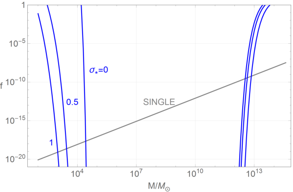
This is just Eq. (2.5) of Ref. [5] with normalized to the mass indicated by the LIGO events. Then, using both the FIRAS limit () [62] and the projected upper limit of for PIXIE [63], the above phenomenological model of non-Gaussianity can be used to calculate the -distortion constraints on or . The results for are presented in Fig. 1; the results for are not shown explicitly, but they have a similar form and can be inferred from Eq. (11). The figure shows that the limits are highly restrictive but much less so in the non-Gaussian cases than the Gaussian one. The PIXIE constraint may no longer be relevant since the project has not been approved. Therefore we give constraints for both PIXIE and a hypothetical future experiment that we dub HYPERPIXIE, assumed to give .
The term in square brackets in Eq. (9) peaks with a value of at , which corresponds to a mass , so the distortion is most sensitive to modes on this scale and has a value . For , this implies for . Hence the decimal logarithm of the PBH formation probability in the Gaussian case, given by Eq. (6), formally reaches . Although this limit is very strong, there is also a value of which corresponds to having just one PBH per current Hubble horizon. This has been described as the “incredulity limit” [71] and can be written as
| (12) |
where is the current horizon mass,
| (13) |
The limit can be well below this, so we also plot in the figures for comparison.
Figures 2 and 3 show the corresponding results for the quadratic and cubic non-Gaussianity investigated in the context of PBHs in Refs. [73, 35]:
| (14) |
| (15) |
The dispersion is then related to via
| (16) |
| (17) |
For each or and mass , which can be translated into , the dispersion (or equivalently ) corresponding to the upper limit on is obtained. The corresponding value of can then be obtained using Refs [73, 35], which leads to Figs. 2 and 3. The limits for cubic non-Gaussianity are weaker than those for quadratic non-Gaussianity, and the limits for type non-Gaussianity are even weaker for sufficiently small . As noted in Ref. [35], in the limit ,we have
| (18) |
where denotes the complementary error function. In the limit , we have
| (19) |
These relations and Eqs. (9) and (10) lead to the curves of Figs. 2 and 3 with and , which serves as a check.


III Discussion
Although we have focused mainly on the distortions associated with PBH formation, we should also comment briefly on the distortions, which can be calculated using Eq. (9b) in Ref. [70] and assuming [62]. It is clear from Fig. 4, which shows the and limits for FIRAS with different values of , that there is a transition at around above which the constraint dominates. This scale is independent of the value of and can be understood from the qualitative discussion at the start of Sec. II. The curves are interesting, even if one does not expect PBHs larger than in practice. Note that including other sources of distortion would merely strengthen the PBH limits. Indeed, HYPERPIXIE will be looking for the signal from astrophysical sources at the level of to , and such a signal will be obscured if the from Silk damping exceeds this. The total constraint for given comes from the combination of the and limits. The value of at the intersect gives a local maximum in the constraint, but there are extended minima on either side of this, with the limit being somewhat weaker than the limit. The value of at the maximum decreases as increases. For , the constraints would be even tighter than in the Gaussian case.

At the present epoch we require SMBHs with mass in galactic nuclei, and the Magorrian scaling implies [75]. If there were no accretion, the PBH scenario would be excluded by the above analysis unless were as low as or and as high as 5000. However, the values of and indicated in Figs. 1-4 correspond to the formation epoch of the PBHs, and the production of SMBHs in galactic nuclei probably requires a very large accretion factor. For example, for Eddington-limited growth, the initial seed mass could be a smaller by a factor of , corresponding to an initial of . If the final mass is much larger than the initial mass, one expects , so the value of (,) in Figs. 1-4 evolves along a straight line. More generally, since the limit is only important above , one could circumvent it altogether, provided the mass increases by a factor . However, in this case the accretion of gas onto the PBHs may also contribute to temperature and polarization anisotropies and distortions of the CMB [19, 20, 74], so accretion may not save the scenario.
The above analysis has considered the types of non-Gaussianity associated with the parameters , and , so it may be useful to comment on the connection between these. The parameter changes the exponential falloff of the PDF, so that it declines as rather than , as in the Gaussian case. This is slower than the Gaussian decline for , so for fixed this widens the PDF but lowers the central height since area is conserved. For and the same value of , the modified curve goes above the Gaussian curve at a value of less than the critical value required for PBH formation, so PBH production will be increased. This explains why the constraints on become weaker as decreases below 2. Of course, this is a particularly simple type of non-Gaussianity, and we do not currently know what kind of physics in the early Universe would lead to it; thus, this is just a convenient phenomenological toy model. Nevertheless, this illustrates qualitatively why the deviations from Gaussianity that we have investigated weaken the PBH constraints.
The parameters and are more traditional measures of non-Gaussianity, whose significance is well understood. From Eq. (14), couples with , so that the average is zero, while couples with from Eq. (15). In principle, one could combine Eqs. (14) and (15) into a single equation to allow and to vary together. Generally a pure can yield either a weaker or stronger constraint than some mixture of and , depending on their precise values. The relative effects of , and are shown in Fig. 5, where the values of as functions of the non-Gaussian parameters are compared for , corresponding to for .

It should be stressed that there are many other types of non-Gaussianity, so the above analysis should only be regarded as demonstrating the importance of this property in principle for the form of the constraint on PBHs. In particular, Ref. [60] discusses an inflationary scenario – termed the patch model – which can produce a sufficient number of PBHs to account for the observed high-redshift quasars, while keeping sufficiently small to evade constraints from distortions. This model is highly non-Gaussian and essentially introduces a spike in the PDF. This form of non-Gaussianity is very different from the types investigated here, so we have not tried to relate them.
Although we have assumed a delta-function primordial power spectrum, we can generalize our analysis to the more plausible situation in which the fluctuations have an extended power spectrum. As a first step, let us consider the following power spectrum:
| (20) |
This reduces to the delta-function spectrum in the limit The distortion can then be calculated using the formalism of Ref. [70] and, for each and , the value of corresponding to the upper limit on can be obtained. In the Gaussian case, is calculated using Eq. (6), and we translate this to using the correspondence between and implied by Eq. (10). The upper limit on so obtained is plotted in Fig. 6. The limits for () are tighter when is larger, due to the additional presence of modes with () which contribute to relatively efficiently but are absent in the corresponding case for a delta-function spectrum.
This is distinct from the effect of an extended PBH mass function, which may arise even for a delta-function power spectrum if one has critical collapse [9]. In this case, one needs to consider which value of dominates the distortion. This depends upon the form of the PBH mass function; however, the limit will be important whenever this extends above , and it will be strongest if it extends up to . The two most plausible mass functions are lognormal (which applies for a large class of inflationary scenarios) and a steeply rising power law with an exponential upper cutoff (which applies for critical collapse). In the first case the mass function only extends over a few decades of mass, so the above analysis is still a reasonable guide. In the second case, the mass function is essentially monochromatic since the number of PBHs on the power-law tail is very small. If the mass function has a power-law form, so that it is very extended, the situation is more complicated, but this is less likely to apply in any realistic scenario. As discussed in Ref. [77], all the constraints on - not just the constraints - are modified anyway for an extended PBH mass function, but we do not consider this complication further here.
IV SUMMARY
PBH formation is a plausible process in the very early Universe. It is motivated observationally by the need for dark matter and by LIGO observations, and theoretically by generic inflationary fluctuation considerations. An inevitable consequence of PBH formation is that the dissipation of primordial fluctuations is also expected to be large. We have developed alternative formalisms for studying primordial non-Gaussianities in these fluctuations and evaluated the associated limits on . Our formalism is equivalent to the more conventional approach in other recent studies of PBH formation from non-Gaussian fluctuations [73]. We have demonstrated that Silk damping could produce unacceptably large distortions of the cosmic microwave background since the fluctuations with wave numbers corresponding to the PBH masses under consideration are expected to dissipate during the redshift interval . We have explored current and future constraints on these distortions and shown how they can be translated into upper limits on the PBH abundance over a wide mass range.
Acknowledgements.
We thank T. Harada, M. Kamionkowski, K. Kohri, V. Poulin, A. Vilenkin, J. Yokoyama and an anonymous referee for helpful input. T.N. and B.C. thank the Research Center for the Early Universe (RESCEU) at the University of Tokyo and the Institut Astrophysique de Paris for hospitality received during this work. T.N. was supported by JSPS Postdoctoral Fellowships for Research Abroad and J. S. by European Research Council Grant No. 267117.References
- [1] Ya. B. Zel’dovich and I. D. Novikov, Sov. Astron. 10, 602 (1967).
- [2] S. Hawking, Mon. Not. Roy. Astron. Soc. 152, 75 (1971).
- [3] B. J. Carr and S. W. Hawking, Mon. Not. Roy. Astron. Soc. 168, 399 (1974).
- [4] S. W. Hawking, Commun. Math. Phys. 43, 199 (1975).
- [5] B. J. Carr, K. Kohri, Y. Sendouda and J. Yokoyama, Phys. Rev. D 81, 104019 (2010).
- [6] G. F. Chapline, Nature (London) 253, 251 (1975).
- [7] A. Barrau , D. Blais, G. Boudoul and D. Polarski, Ann. Phys. (Berlin) 13, 115 (2004).
- [8] S. Clesse and J. Garcia-Bellido, Phys. Rev. D 92, 023524 (2015).
- [9] B. J. Carr, F. Kuhnel and M. Sandstat, Phys. Rev. D 94. 044029 (2016).
- [10] P. H. Frampton, Mod. Phys. Lett. A 31, 1650093 (2016).
- [11] R. H. Cyburt, B. D. Fields and K. A. Olive, Phys. Lett. B 567, 227 (2003).
- [12] E. Di Valentino, E. Giusarma, M. Lattanzi, A. Melchiorri and O. Mena, Phys. Rev. D 90, 043534 (2014).
- [13] C. G. Lacey and J. P. Ostriker, Astrophys. J. Lett. 299, 633L (1985).
- [14] R. Bean and J. Magueijo, Phys. Rev. D 66, 063505 (2002).
- [15] M. Kawasaki, A. Kusenko and T. T. Yanagida, Phys, Lett. B 711 1 (2012).
- [16] B. J. Carr and J. Silk, “Primordial black holes as seeds for cosmic structure”, preprint (2017).
- [17] N. Afshordi, P. McDonald and D. N. Spergel, Astrophys. J. Lett. 594, L71 (2003).
- [18] A. Kashlinksy, Astrophys. J. 823, L25 (2016).
- [19] M. Ricotti, J. P. Ostriker and K. J. Mack, Astrophys. J. 680, 829 (2008).
- [20] Y. Ali-Haïmoud and M. Kamionkowski, Phys. Rev. D 95, 043534 (2017).
- [21] G. M. Fuller, A. Kusenko and V. Takhistov, Phys. Rev. Lett. 119, 061101 (2017).
- [22] S. Bird, I. Cholis, J. B. Muñoz, Y. Ali-Haïmoud, M. Kamionkowski, E. D. Kovetz, A. Raccanelli and A. G. Riess, Phys. Rev. Lett. 116, 201301 (2016).
- [23] M. Sasaki, T. Suyama, T. Tanaka and S. Yokoyama, Phys. Rev. Lett. 117, 061101 (2016).
- [24] J. R. Bond and B. J. Carr, Mon. Not. Roy. Astron. Soc. 207, 585 (1984).
- [25] T. Kinugawa, K. Inayoshi, K. Hotokezaka, D. Nakauchi and T. Nakamura, Mon. Roy. Astron. Soc. 442, 2963 (2014).
- [26] B. J. Carr, Astron. Astrophys. 89, 6 (1980).
- [27] T. Nakamura, M. Sasaki, T. Tanaka and K. S. Thorne, Astrophys. J. Lett. 487, L139 (1997).
- [28] A. M. Green, Phys. Rev. D 94, 063530 (2016).
- [29] F. Kuhnel and K. Freese, Phys. Rev. D 95, 083508 (2017).
- [30] B. J. Carr, M. Raidal, T. Tenkanen, V. Vaskonen and H. Veermäe, Phys. Rev. D 96, 023514 (2017).
- [31] B. J. Carr, Astrophys. J. 201, 1 (1975).
- [32] R. H. Cyburt and B. Davids, Phys. Rev. C 78, 064614 (2008).
- [33] D. P. Quinn, M. I. Wilkinson, M. J. Irwin, J. Marshall, A. Koch, and V. Belokurov, Mon. Not. R. Astron. Soc. Lett. 396, L11 (2009).
- [34] M. A. Monroy-Rodríguez and C. Allen, Astrophys. J. 790, 159 (2014).
- [35] T. Nakama, J. Silk and M. Kamionkowski, Phys. Rev. D 95, no. 4, 043511 (2017).
- [36] García-Bellido J., Peloso M., Unal C., JCAP, 9, 013 (2017).
- [37] B. J. Carr, in Inflating Horizons in Particle Astrophysics and Cosmology, edited by H. Susuki et al. (Universal Academy Press, Tokyo, 2005), pp. 119-149.
- [38] M. Y. Khlopov and A. G. Polnarev, Phys. Lett. 97B, 383 (1980).
- [39] K. Jedamzik, M. Lemoine and J. Martin, JCAP 1009, 034 (2010).
- [40] T. Harada, C. M. Yoo, K. Kohri, K. i. Nakao and S. Jhingan, Astrophys. J. 833, no. 1, 61 (2016).
- [41] B. J. Carr, T. Tenkanen and V. Vaskonen, Phys. Rev. D 96, 063507 (2017).
- [42] P. Ivanov, P. Naselsky and I. Novikov, Phys. Rev. D 50, 7173 (1994).
- [43] J. Yokoyama, Astron. Astrophys. 318, 673 (1997).
- [44] J. S. Bullock and J. R. Primack, Phys. Rev. D 55, 7423 (1997).
- [45] J. Yokoyama, Phys. Rev. D 58, 083510 (1998).
- [46] M. Kawasaki, A. Kusenko, Y. Tada and T. T. Yanagida, Phys. Rev. D 94, 083523 (2016).
- [47] M. Kawasaki, and Y. Tada, JCAP, 8, 041 (2016).
- [48] P. H. Frampton, M. Kawasaki, F. Takahashi, and T. T. Yanagida, J. Cosmol. Astropart. Phys. 04 023 (2010).
- [49] J. Garriga, A. Vilenkin and J. Zhang, JCAP 1602, no. 02, 064 (2016).
- [50] H. Deng and A. Vilenkin, arXiv:1710.02865 (2017).
- [51] A. D. Dolgov, arXiv:1605.06749 (2016).
- [52] J. Kormendy and D. Richstone, Ann. Rev. Astron. Astrophys. 33, 581 (1995).
- [53] F. Hoyle and J.V. Narlikar, Proc. R. Soc. London A 290, 177 (1966).
- [54] P. Meszaros, Astron. Astrophys. 38, 5 (1975).
- [55] J. Silk, Astrophys. J. 151, 459 (1968).
- [56] B. J. Carr and J. E. Lidsey, Phys. Rev. D 48 543 (1993).
- [57] J. D. Barrow and P. Coles, Mon. Not. Roy. Astron. Soc. 248, 52 (1991).
- [58] J. Chluba, J. Hamann and S. P. Patil Int. J. Mod. Phys. D 24, no. 10, 1530023 (2015).
- [59] K. Kohri, T. Nakama and T. Suyama, Phys. Rev. D 90, no. 8, 083514 (2014).
- [60] T. Nakama, T. Suyama and J. Yokoyama, Phys. Rev. D 94, no. 10, 103522 (2016).
- [61] K. Inomata, M. Kawasaki, K. Mukaida, Y. Tada and T. T. Yanagida, Phys. Rev. D 95, no. 12, 123510 (2017).
- [62] D. J. Fixsen, E. S. Cheng, J. M. Gales, J. C. Mather, R. A. Shafer and E. L. Wright, Astrophys. J. 473, 576 (1996).
- [63] M. H. Abitbol, J. Chluba, J. C. Hill and B. R. Johnson, Mon. Not. Roy. Astron. Soc. 471, 1126 (2017).
- [64] T. Nakama, T. Suyama and J. Yokoyama. Phys. Rev. Lett. 113, 061302 (2014).
- [65] H. Tahsiro and N. Sugiyama, Phys. Rev. D 78, 023004 (2008).
- [66] T. Nakama, T. Harada, A. G. Polnarev and J. Yokoyama, JCAP 01, 037 (2014).
- [67] T. Harada, C. M. Yoo, K. Kohri and K. I. Nakao, Phys. Rev. D 96, no. 8, 083517 (2017).
- [68] T. Harada, C. M. Yoo, T. Nakama and Y. Koga Phys. Rev. D 91, 084057 (2015).
- [69] S.Young, C.T. Byrnes and M, Sasaki, JCAP 1407 (2014) 045; arXiv:1405.7023
- [70] J. Chluba, A. L. Erickcek and I. Ben-Dayan, Astrophys. J. 758, 76 (2012).
- [71] B. J. Carr and M. Sakellariadou, Astrophys. J. 516, 195 (1999).
- [72] P. A. R. Ade et al. [Planck Collaboration], Astron. Astrophys. 594, A13 (2016).
- [73] C. T. Byrnes, E. J. Copeland and A. M. Green, Phys. Rev. D 86, 043512 (2012).
- [74] V. Poulin, P. D. Serpico, F. Calore, S. Clesse and K. Kohri, arXiv:1707.04206 (2017).
- [75] N.J. McConnell and C.-P. Ma, Astrophys. J. 764, 184 (2013).
- [76] A. Soltan, Mon. Not. Roy. Astron. Soc. 200, 115 (1982).
- [77] B.J. Carr, M. Raidal, T. Tenkanen, V. Vaskonen and H. Veermae, Phys. Rev. D. 96, 023514 (2017).