Weighted Tensor Decomposition for
Learning Latent Variables with Partial Data

Omer Gottesman ^†^†thanks: gottesman@fas.harvard.edu Affiliation: Paulson School of Engineering and Applied Sciences, Harvard University Weiwei Pan Affiliation: Paulson School of Engineering and Applied Sciences, Harvard University Finale Doshi-Velez ^†^†thanks: finale@seas.harvard.edu Affiliation: Paulson School of Engineering and Applied Sciences, Harvard University

Abstract

Tensor decomposition methods are popular tools for learning latent variables given only lower-order moments of the data. However, the standard assumption is that we have sufficient data to estimate these moments to high accuracy. In this work, we consider the case in which certain dimensions of the data are not always observed—common in applied settings, where not all measurements may be taken for all observations—resulting in moment estimates of varying quality. We derive a weighted tensor decomposition approach that is computationally as efficient as the non-weighted approach, and demonstrate that it outperforms methods that do not appropriately leverage these less-observed dimensions.

1 Introduction

Tensor decomposition methods decompose low-order moments of observed data to infer the latent variables from which the data is generated (Anandkumar et al., 2014; Arora et al., 2012). They have recently gained popularity because they require only moments of the data and, in the absence of model-mismatch, come with global optimality guarantees. Of course, these guarantees require that the moments are well-estimated—which corresponds to the amount of available data. Previous works have investigated the dependence of the inference quality on the amount of collected data (and the related uncertainty in the moment estimates) (Anandkumar et al., 2014; Kolda and Bader, 2009; Podosinnikova et al., 2015). However, these works typically assume that every dimension is observed in every datum.

In this work, we consider the scenario in which some dimensions are always observed, while others may be available for only a few observations. Such situations naturally arise in real world applications. In clinical settings, for example, easily obtained measurements such as temperature and blood pressure may be available for all patients, but the results of a blood test may be available for only a small number of patients. Similarly, billing codes may be available for all patients, while information extracted from unstructured notes only for a subset. In biology applications, one may want to combine counts from whole genome sequencing from a smaller study with counts of the subset of SNPs from a larger population.

Let us suppose that we are only interested in latent variable models over the dimensions that are completely observed. In the medical setting example we presented earlier, that would correspond to learning a model to explain only the patients’ temperature and blood pressure data. In such a case, would using the data on other vitals be helpful or detrimental to learning? We demonstrate that depending on the frequency at which a dimension is missing in the data, including its associated estimated moments may help or hinder the estimation of latent variable model parameters for the rest of the model.

Of course, the more interesting question is whether we can do better than sometimes ignoring dimensions with missingness—that is, can the lower quality moment estimates from these incompletely-observed dimensions still be used to improve our inference about the structure of the complete dimensions? We introduce a weighted tensor decomposition method (WTPM) which weights elements in the moment estimates proportionally to the frequency at which they are observed. It has identical computation requirements to the unweighted approach, and performs as well as or better than both unweighted approaches, i.e. including or ignoring the dimensions which are sometimes missing. We present experimental results for two commonly used latent variable models: Gaussian mixtures and the Gamma-Poisson model.

2 Background and Setting

2.1 Tensor decomposition methods

The principle at the heart of learning latent variable models via tensor decomposition is simple: the moments of many such models can be written as a tensor decomposition of the models parameters in the form

	S	$\displaystyle=\sum_{k}s_{k}\textbf{a}_{k}\textbf{a}_{k}^{T},$		(1)
	T	$\displaystyle=\sum_{k}t_{k}\textbf{a}_{k}\otimes\textbf{a}_{k}\otimes\textbf{a}_{k}.$		(2)

Here, $\textbf{a}_{k}$ denotes columns of the parameter matrix $\textbf{A}\in\mathbb{R}^{D\times K}$ , representing the $k^{th}$ latent parameter in a $D$ dimensional space. A can then be inferred from the data - denoted for a dataset of $N$ samples by the matrix $\textbf{X}\in\mathbb{R}^{D\times N}$ - by computing the empirical estimates of the moments $\hat{\textbf{S}}(\textbf{X})$ and $\hat{\textbf{T}}(\textbf{X})$ , and calculating their decomposition. The procedure is quite general and can be applied whenever the expression for the empirical estimates of the moments can be derived and computed from the data. In this work we present results for mixtures of spherical Gaussians (Hsu and Kakade, 2013) and the Gamma-Poisson (GP) model (Podosinnikova et al., 2015). A description of the generative models and the form of the empirical estimates can be found in appendix A.

Several methods exist to estimate the decomposition of the tensor estimates (Hyv et al., 1999; Cardoso and Souloumiac, 1993; Anandkumar et al., 2014). In this work, we use the method described in Anandkumar et al. (2014), which provides a polytime algorithm to learn the parameters from the moment estimates. The method consists of two stages. In the first stage the eigenstructure of $\hat{\textbf{S}}$ is used to compute a whitening matrix, W, which is used to reduce $\hat{\textbf{T}}$ to a $K\times K\times K$ tensor with an orthogonal decomposition, $\hat{\textbf{T}}_{c}$ . In the second stage, the tensor power method (TPM) - the tensor analog of the matrix power method - is used to calculate the eigenvectors of $\hat{\textbf{T}}_{c}$ , which can be transformed into the columns of the parameter matrix $\hat{\textbf{A}}$ using W once again. (For more details see Anandkumar et al. (2014)). We emphasize that our results are not specific to this choice of decomposition method.

Refer to caption — Figure 1: (a) Basic uncorrelated structure of missing data. Colored elements represent missing data elements which are not observed. Specifically, every dimension $d^{th}$ in a sampled data point $x_{n}$ (column $n$ in X) is present with some probability $p_{d}$ , independently of the missingness of all other elements in the data. (b) Correlated missing data structure in the toy example.

2.2 Missingness

In the following, we assume that there exist a certain set of complete dimensions that are always recorded in every observation. It is the relationships between these dimensions that we are most interested in recovering. The remaining incomplete dimensions are missing completely-at-random with probability $(1-p_{d})$ . That is, the probability that one of these dimensions is not recorded in observation $n$ is independent of all other dimensions in $\textbf{x}_{n}$ , the data set X, and the specific value of $x_{nd}$ . A schematic illustration of such a dataset is presented in Figure 1 (a). To calculate $p_{d}$ empirically we simply count the number of samples in which a given dimension is observed, and divide by the number of samples, $N$ .

3 The Value of Incomplete Data: Motivating Example

In Section 1, we asked a simple question: if some of our observations are incomplete—that is, we have observed only a few of the possible dimensions—then is it better to just discard them? Or are there instances in which the additional poorly-estimated moments are valuable for recovering parameters associated with the complete dimensions? In this section, we demonstrate that the answer depends on how poorly estimated those additional moments are—there are regimes in which the additional moments only add noise, and regimes in which they assist with the overall parameter recovery.

We consider a very simple missingness pattern for the purpose of illustration, shown schematically in Figure 1 (b). Specifically, we consider a data set that consists of $N_{f}$ full observations, for which all dimensions are observed, and $N_{p}$ partial observations, for which some dimensions are never observed. (Note that this structure is not missing-at-random, which we will require for our derivations of Lemma 4.1, but makes it simpler to illustrate the idea.)

Our metric for the reconstruction error of the parameter matrix A incorporates only the complete dimensions:

\varepsilon_{c}\equiv\sum_{k}\frac{\hat{\textbf{a}}_{c,k}\cdot\textbf{a}_{c,k}}{||\hat{\textbf{a}}_{c,k}||\cdot||\textbf{a}_{c,k}||},

(3)

where $\textbf{a}_{c,k}$ is the vector comprised only of the complete elements in the $k^{th}$ latent parameter. We measure the reconstruction error as the sum of angles in high dimensional space between the true and inferred parameters in order to avoid ambiguities due to scaling and normalization. (In particular, the columns of A in the GP model are normalized to sum to one, so it is necessary to choose a measure of error which is independent of normalization.)

In our illustration, we use the GP model and consider the recovery of a single topics matrix $\hat{\textbf{A}}\in\mathbb{R}^{10\times 4}$ , shown in Figure 2 (c) (In Appendix D, we demonstrate that our results also hold across a large number of randomly generated topic matrices A).

We consider two options for recovering the parameters corresponding to the complete dimensions, $\textbf{A}_{c}$ . The first, which we call the full dimensionality method, makes use of all the data available. That is, if certain dimensions of an observation $\textbf{x}_{n}$ are missing, we still use the non-missing dimensions to assist in estimating the tensors $\hat{\bf{S}}$ and $\hat{\bf{T}}$ . (See the schematic insets in Figure 3 to see what elements of the second order tensor we take into account when performing the decomposition). Once we have learned the topics for all dimensions, we can observe only the complete dimensions which are of interest.

The full dimensionality method results in decomposing tensors in which each element may have a different uncertainty. In contrast, the second approach—which we call the partial dimensionality method—discards any dimensions that are not always present in the data and performs the inference on the lower dimensional problem consisting of only the elements which are always observed. Tensor elements in the partial dimensionality method will have equal uncertainties, but will include fewer correlations.

In Figure 2, we provide some intuition for the factors affecting the performance of the two methods. In Figure 2 (a) we illustrate the effect of using only a subset of the dimensions for inference. Our goal is to infer the topic structure of six out of the ten dimensions in the data. To perform such inference, we must use the dimensions whose structure we try to infer, but may ignore some of the other dimensions. Figure 2 (a) demonstrates that for a given number of samples, ignoring the extra dimensions leads to larger inference error, as important information about the structure of the data is ignored.

To contrast the simple case where no data is missing, in Figure 2 (b), we demonstrate the effect of partial data on the topics recovery error. We present the reconstruction error using the full dimensionality method where for $N_{f}$ full samples all the dimensions in the data are observed, and for $N_{p}$ partial samples only 6 of the 10 dimensions are observed in the data. These partial data allow us to better estimate the moments associated only with those 6 dimensions, but the error in the remaining moments is not reduced by these additional observations. The relatively flat lines suggest that the recovery error is dominated by the moments with the highest uncertainty—something that the partial data cannot fix—and therefore collecting additional partial data does little to improve the inference of the full dimensionality method.

Finally, in Figure 3, we plot the reconstruction error as a function of $N_{p}$ at a constant $N_{f}$ for both the full dimensionality and the partial dimensionality methods. As seen in Figure 2 (b), additional partial samples do not help the full dimensionality method, which is dominated by the least accurate tensor elements. In contrast, with the partial dimensionality method, the topics reconstruction error steadily decreases, as the estimates $\hat{\bf{S}}$ and $\hat{\bf{T}}$ converge to their true value (and as long as that subset of the true topics matrix A associated with those dimensions satisfies the incoherence requirements in Anandkumar et al. (2014), $\hat{\textbf{A}}_{c}$ will converge to $\textbf{A}_{c}$ ). However, for small amounts of partial data, because we are effectively working on data with lower dimensionality, our reconstruction error is worse compared to the results of the full dimensionality model—or put another way, when all the tensor elements have similar uncertainties, it makes sense to use all the correlations that we have available. The existence of this cross-over suggests an opportunity for an algorithm that can attain the better recovery in all cases. We derive such an algorithm in Section 4.

4 The Weighted Tensor Power Method (WTPM)

In Section 3, we demonstrated that the choice of whether to use the dimensions with missing data depends on the relative quality of the moment estimates. In section 3 we gave an intuition for why if the dimensions with missing data did not have significantly less data than the dimensions with complete data, it would make sense to include those moments in order to get a more complete correlation structure of the data. However, since the quality of the inference is dominated by the noisiest tensor elements, it does not make sense to include tensor elements that may be of significantly lower quality—as would be the case if the dimensions with missing data had significantly less data associated with them than the complete dimensions.

In this section we introduce the Weighted Tensor Power Method (WTPM) for spectral learning with missing data. It is more general than the motivating example in Section 3 in that we allow different dimensions to have different levels of missingness, but we shall also need to require that each dimension is missing at random. (This assumption is required for our derivation. We will show that our approach is robust to other missingness structures in Section 5.1). The key idea behind our approach is the intuition that we would like to use all the moments of the data, but assign higher importance to moments for which we have smaller uncertainties. A natural and intuitive way to perform this task is by performing tensor decomposition on weighted tensors. The weighting consists of multiplying every element in the empirical tensor estimates, $\hat{\bf{S}}$ and $\hat{\bf{T}}$ , by some weight which represents the importance we give that specific element. Thus, the elements of the weighted tensors, $\hat{\bf{S}}^{*}$ and $\hat{\bf{T}}^{*}$ , are given by

	$\displaystyle\hat{S}_{d_{1}d_{2}}^{*}$	$\displaystyle=w_{d_{1}d_{2}}\hat{S}_{d_{1}d_{2}}$		(4)
	$\displaystyle\hat{T}_{d_{1}d_{2}d_{3}}^{*}$	$\displaystyle=w_{d_{1}d_{2}d_{3}}\hat{T}_{d_{1}d_{2}d_{3}}.$		(5)

To apply the efficient algorithms of standard tensor decomposition methods, the weighting scheme must also maintain the structure of the tensors as sums of $K$ rank 1 tensors, similar to moment equations (1) and (2). To maintain such a structure, we write the weights as a product of the weights associated with every dimension contributing to the tensor:

\displaystyle\begin{split}w_{d_{1}d_{2}}&=w_{d_{1}}w_{d_{2}}\\ w_{d_{1}d_{2}d_{3}}&=w_{d_{1}}w_{d_{2}}w_{d_{3}}.\end{split}

(6)

This weighting scheme allows us to rewrite the moments as

	$\displaystyle S_{d_{1}d_{2}}^{*}$	$\displaystyle=w_{d_{1}d_{2}}S_{d_{1}d_{2}}=\sum_{k}s_{k}w_{d_{1}d_{2}}a_{d_{1}k}a_{d_{2}k}$
		$\displaystyle=\sum_{k}s_{k}(w_{d_{1}}a_{d_{1}k})(w_{d_{2}}a_{d_{2}k})=\sum_{k}s_{k}a_{d_{1}k}^{}a_{d_{2}k}^{}.$

where we defined $a_{dk}^{*}=a_{dk}w_{d}$ . An analogous expression can be written for the third-order tensor $T^{*}$ . Written in this form, it is clear that the weighted tensors also have the structure of a sum of $K$ rank 1 tensors, and therefore can be decomposed using standard tensor decomposition methods.

This form of the weights enjoys the additional advantage of allowing us to view the weighting of the moments tensors as a rescaling of the dimensions in the topics and data, $x_{dn}^{*}=x_{dn}w_{d}$ and $a_{dk}^{*}=a_{dk}w_{d}$ , providing an intuitive explanation for the effect of weighting the moments. This view also allows us to perform the weighting on the data itself, multiplying each dimension by $w_{i}$ , rather than on the moments.

Finally, once we perform the decomposition and learn the rescaled topic matrix, we can rescale this matrix back by dividing its $d^{th}$ row by $w_{d}$ to reconstruct the entire topic matrix, and not just the part corresponding to the complete dimensions. However, this full reconstruction is very susceptible to noise as error in reconstructing the incomplete dimensions will be amplified when dividing by the small weights associated with them.

Running Time

A consequence of viewing the weighting as a rescaling of the data is that the WTPM has the same running time as a standard tensor decomposition method, as it can be implemented by scaling each dimension of the data by $w_{d}$ and then applying one’s tensor decomposition method of choice.

Choice of Weights

The question remains of what weights $w_{d}$ to assign to each dimension. Our approach is to choose weights that minimize the inference error. In this way, optimal weights can be computed for any model for which one can derive expressions for the inference error as a function of moment estimations errors and any other parameters affected by the weighting.

Demonstrating our approach, we first present the choice of optimal weights for the Gamma-Poisson model. Podosinnikova et al. (2015) drew and expanded on sample complexity bounds results from Anandkumar et al. (2012) to show that the inference error has two main contributions, one which scales as $\mathbb{E}\left[||\hat{\textbf{S}}-\textbf{S}||_{F}\right]/L^{2}$ , and one which scales as $\mathbb{E}\left[||\hat{\textbf{T}}-\textbf{T}||_{F}\right]/L^{3}$ . By choosing our weights to minimize these two ratios we can derive the weights which minimize the topics reconstruction error:

Lemma 4.1.

Assume that the magnitude of all elements in $\bf{A}$ are comparable, and that the probabilities of elements in the data to be missing are independent of each other. For high dimensional problems, an intuitive upper bound $\phi(\mathbf{w})$ , of the expected topic reconstruction error, $E_{\mathrm{infer}}$ , under the GP model is locally minimized by setting:

\displaystyle w_{d}\propto p_{d},

where $p_{d}$ is the probability of an element in the $d^{th}$ dimension to be observed in the data.

Proof.

The upper bound $\phi(\mathbf{w})$ on $E_{\mathrm{infer}}$ is essentially the sum of the Jensen gaps of the expected sampling errors, $\mathbb{E}\left[||\hat{\textbf{S}}-\textbf{S}||_{F}\right]$ and $\mathbb{E}\left[||\hat{\textbf{T}}-\textbf{T}||_{F}\right]$ .

See Appendix E for details.

An immediate corollary of Lemma 4.1 is that weighting the dimensions according to degrees of missingness is provably better for inference than the unweighted model. In Appendix E, we show that under stronger assumptions, where we neglect the structure in the data, we can obtain globally optimal weighting by the choice $w_{d}\propto\sqrt{p_{d}}$ . But in experimentation, we find the performance of both to be indistinguishable.

We note that in our actual WTPM we choose not to rescale the complete dimensions, thus we simply set the proportionality constant to 1 and use the scaling $w_{d}=p_{d}$ . In practice, we find that choosing the weights according to Lemma 4.1 yields good results even when there is a large variance in the magnitude of the elements of $\bf{A}$ .

Additionally, we find that the weighting proposed in Lemma 4.1 leads to good inference results for most models, including Gaussian mixtures. Thus, in many cases, one may forgo derivations involving analytical expressions for the inference error in favor of the the heuristic of choosing $w_{d}=p_{d}$ . For example, while inference error bounds (in terms of the weights) exist for Gaussian Mixtures, the necessary conditions for these bounds to hold render optimization intractable.

Finally, we note that the mixture of Gaussians also requires an estimation of the variance, and reweighing dimensions will change a spherical Gaussian into an elliptical one. We provide details on how the weighting affects the variance estimation process in appendix C.

5 Results

In this section we compare our WTPM with the full and partial dimensionality methods described in Section 3. We test our method on synthetic, semi-synthetic, and real data sets for different structures of missing data and show that in all cases the WTPM interpolates between the more naive methods, always performing as well as or better than the best of them.

5.1 Synthetic Examples

Gaussian Mixtures

Figure 4 (left) compares the WTPM with the full and partial dimensionality methods for synthetic data of Gaussian mixtures with $D=10$ , $K=4$ and $4$ missing dimensions. The inference error for the complete dimensions, $\varepsilon_{c}$ is plotted vs. the number of samples, $N$ . Each sub-figure shows the results for a different missingness pattern, given as a vector, $\bf{p}$ , representing the probability of each dimension to be present in the data. The first six dimensions in each instance are complete dimensions and are always observed ( $p=1$ ), and the last four incomplete dimensions are present in the data with different probabilities. The centers of all Gaussians were sampled from a normal distribution $A_{ij}\sim\mathcal{N}(0,100)$ for all $(i,j)$ , and the variance of the spherical Gaussians is $\sigma^{2}=100$ . $\boldsymbol{\pi}$ was sampled from a Dirichlet distribution, $\boldsymbol{\pi}\sim\text{Dir}(\bf{1})$ . In all cases, the WTPM always did as well as or better than both the full and partial dimensionality method. We emphasize that because in some instances the partial dimensionality method outperforms the full dimensionality method and in some instances the opposite is true, always matching the best of the two methods with one algorithm is already advantageous, even when the WTPM does not outperform the two other methods.

Gamma-Poisson

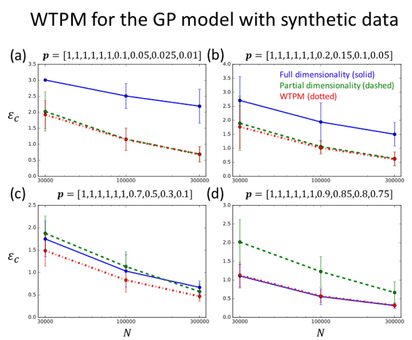
Next, we investigate the performance of our WTPM and compare it to the performance of the full and partial dimensionality methods for data generated from the topics presented in Figure 2. In Figure 4 (right) we present results for experiments on four different choices of missingness patterns, given by the vector p. When the incomplete dimensions are missing with high probabilities (small $p$ for the incomplete elements, Figure 4 (a-b)), the moments including the incomplete dimensions are very noisy and including them in the inference by using the full dimensionality method (blue) leads to a higher reconstruction error compared with the partial dimensionality method (green). The opposite is true when the incomplete dimensions are missing with low probability (large $p$ for the incomplete elements, Figure 4 (d)) and the full dimensionality method performs better by using the additional correlations which are less noisy in this case.

As with the Gaussian mixtures, the WTPM (red) does as well as or better than the best of the two baselines in all cases. In cases where values of $p$ for the incomplete dimension are distributed over a wide range of values (Figure 4 (c)), the WTPM significantly outperforms both other methods, as it optimizes the amount of information in every moment, while properly down-weighting each moment according to its uncertainty.

Finally, in Figure 5(a), we present results based on the missingness pattern in Figure 1(b) and the synthetic model in Figure 3, where all partial dimensions are either present or missing together. This missingness violates the assumptions required in Lemma 4.1, the WTPM is robust to this violation and outperforms both full and partial dimensionality methods in this case as well.

5.2 Semi-synthetic Examples: 20 Newsgroups and Autism Comorbidities

To investigate the effect of incomplete dimensions within the kinds of sparse topic structure found in real data, we adopt a similar approach to Arora et al. (2013) and run still carefully-controlled experiments on semi-synthetic data. We use two real data sets to create semi-synthetic data for the WTPM: word counts from 4 categories of the 20-Newsgroups collection of news documents (Mitchell, 1997), filtered for words which appear in at least $5\%$ of the documents ( $D=175$ , $K=4$ , original $N=3,652$ ); and counts of 64 common diagnoses from a collection electronic health records of children with autism at ages 5 and 10 (Doshi-Velez et al., 2014) ( $D=128$ , $K=5$ , original $N=5,475$ ).

To create the semi-synthetic data from these data, we first run a standard tensor decomposition on a real dataset to learn the parameters of a GP model (D, c and $b$ ), mimicking the sparse data structure common to real world applications. To create the missing data structure, we first chose a set of missing dimensions for each data set. For the ASD data we chose the 64 dimensions corresponding to observations of symptoms at age 5. For the 20-Newsgroups data we randomly chose 116 out of the 175 dimensions. For each one of the incomplete dimensions, $p_{d}$ was sampled uniformly between 0 to 0.9, resulting in a complicated structure of incomplete dimensions, with some dimensions missing in an insignificant amount of data, and some dimensions nearly completely unobserved. We emphasize that while the original data sets used to learn the topics are small, the semi-synthetic data set is large, allowing us to test the performance of our algorithm for a large amount of data.

Figure 5 compares the WTPM with the full and partial dimensionality methods for the semi-synthetic data and a random structure of missingness in the data. The WTPM performs as well or better than both the full and partial dimensionality method across the entire wide range of missingness patterns tested.

5.3 Real Data Example: Sepsis ICU data

As a final demonstration of the WTPM, we use the method to learn the structure of data on sepsis patients collected in ICUs. The data is obtained from the Medical Information Mart for Intensive Care III (MIMIC-III) database (Johnson et al., 2017). The database contains more than 18,000 patients, and every patient’s vitals were sampled on average at 14 different times, resulting in about 250,000 samples. Each sample is represented as a 47 dimensional vector containing information on a patient such as the vitals, lab results, demographics, etc. We wish to learn the structure of the data by modeling it as a mixture of Gaussians. The data collected in the ICU is often incomplete, and the missingness rate for different dimensions ranges from 0 to 0.75, making it an ideal dataset to test with our WTPM. We define as complete dimensions all the dimensions whose missingness rate is smaller than 0.05, resulting in 24 complete dimensions. We learn a mixture of Gaussian model for the complete dimensions with $K=6$ topics using the full and partial dimensionality methods, as well the WTPM.

In Figure 6 we demonstrate that the WTPM performs as well as the full dimensionality method, which performs significantly better than the partial dimensionality method. The WTPM performs well despite the noisiness of the data: the missingness rate spans a wide range of values across different dimensions and is non-zero even for most of the dimensions we define as complete. Furthermore, given the nature of data collection in the ICU, we believe the missingness pattern is likely to be strongly correlated; the WTPM is robust to these assumption violations.

6 Discussion

The derivation of the ideal weights presented in Lemma 4.1 assumes the missingness of different elements is uncorrelated, and also ignores the structure of the topics matrix. However, we have demonstrated that the WTPM is robust to violations of these assumptions: Figure 5 demonstrates that the WTPM method works with a perfectly correlated missingness pattern (an element is missing in a sample if and only if all other incomplete dimensions in the sample are missing). The effectiveness of the WTPM on the semi-synthetic data generated from sparse topics matrices with significant magnitude differences between their non-zero elements demonstrates the insensitivity to the structure of the topics matrix. In future work, it would be interesting to check whether the effectiveness of the WTPM can be further improved by taking into account the structure of the topics and correlations in the missingness. For example, taking into account the structure of the data could mean that it would be advantageous to weight differently dimensions which on average have higher values compared with other dimensions.

While we focused on Gaussian mixtures and the gamma-Poisson model in this work, the core idea behind the WTPM can be applied to method-of-moment-based inference for other models as well. The form of the sample complexity bounds for LDA (Anandkumar et al., 2012), HMM (Hsu et al., 2012) and other topic models such as correlated topic models and Pachinko allocation (Arora et al., 2013; Blei and Lafferty, 2007; Li and McCallum, 2006) are quite similar to the bounds calculated by Podosinnikova et al. (2015), and we therefore expect the application of the WTPM to these models to only require a derivation similar to that presented in Appendix E.

Another interesting direction is asking what we can say about the parameters of the dimensions that are incompletely observed. In this work, we demonstrated that lower-quality moment estimates from the incomplete dimensions could assist with the recovery of the parameters associated with the complete dimensions. The WTPM approach does give us values for all of the parameters—including ones associated with incomplete dimensions. These parameters can be straightforwardly up-weighted by $\frac{1}{w_{d}}$ to get parameter-values for the original data scaling. However, if those parameters are poorly estimated—which is likely, if their associated moment estimates were poor—this rescaling will not result in smaller errors compared with a standard tensor decomposition approach. It is an open question if it is possible to get better recovery of these parameters as well.

Finally, we note that given an implementation of the tensor power method described in Anandkumar et al. (2014), performing the WTPM is very straightforward, and requires only multiplying the empirical estimates $\hat{\textbf{S}}$ and $\hat{\textbf{T}}$ by $\textbf{p}\otimes\textbf{p}$ and $\textbf{p}\otimes\textbf{p}\otimes\textbf{p}$ respectively, before performing the decomposition. In practice, $\hat{\textbf{T}}$ is frequently not calculated explicitly in order to avoid a cubic dependence of the runtime on the dimensionality. Rather, it is possible to use an implicit calculation of $\hat{\textbf{T}}$ that reduces the runtime to $O(DK+nnz(\textbf{X}))$ , where $nnz(\textbf{X})$ is the number of non-zero elements in X (Zou et al., 2013). However, the method proposed in Zou et al. (2013), as well as other methods which do not explicitly calculate $\hat{\textbf{T}}$ can only work when there are no missing elements in the data. While the explicit calculation of the third moments does not scale well with dimensionality of the data, its runtime is independent of document length once the data is converted into word-count format, and should therefore out-perform inference methods such as Gibbs-sampling for data consisting of very long documents.

7 Related Work

Tensor decomposition has been studied for nearly a century, but has recently gained popularity within many different scientific communities (Kolda and Bader, 2009). In particular, a series of works have shown that tensor decomposition methods can recover the parameters of many classes of latent variable models (Anandkumar et al., 2014; Arora et al., 2012; Collins and Cohen, 2012; Zou et al., 2013; Parikh et al., 2011; Podosinnikova et al., 2015). These works generally provide connections between the quality of the moment estimates and the model parameter estimates as a step toward deriving high-probability bounds on the quality of model parameter estimates; however, none of them address the question of what to do when moment estimates are of only moderate and unequal quality.

More broadly, it is well-known that decompositions of empirical moments may result in model parameter estimates that are far from the maximum-likelihood parameter values, especially in the presence of model mismatch. Zhang et al. (2014) and Shaban et al. (2015) both show that in certain circumstances, using the spectral parameter estimates as initialization for an optimization procedure can result in the discovery of the true maximum-likelihood parameter settings. Tran et al. (2016) use an M-estimation framework to regularize the parameter estimates. In the specific case of HMMs, Huang and Schneider (2013) show how to combine cross-sectional and sequence data to produce better parameter estimates. Cheng et al. (2015) investigate the effect uncertainties in the second order tensor elements have on its spectral structure in order to bound the numbers of topics. Again, none of these works address inference in the presence of unequal quality moment estimates.

Finally, there exists a large literature relating to algorithms for tensor decompositions. Jain and Oh (2014) discuss decompositions when tensor elements are missing, distinct from our case in which certain dimensions are not always recorded. Weighted matrix factorization methods such as Srebro et al. (2003), are closely related in spirit to the algorithm we presented and perform a weighted decomposition of higher order tensors.

8 Conclusion

In this work, we derived and presented the Weighted Tensor Decomposition Method (WTDM) for method-of-moment inference in latent variables with missing data. In situations where some dimensions are incompletely observed, we show that we can still leverage the associated low quality moment estimates to get better parameter estimation than simply ignoring that information, while minimizing inference errors due to moments that are too noisy. Our method is easy to implement and enjoys the same large-sample recovery guarantees as standard tensor decomposition-based inference methods; we demonstrate its benefits for two models and our derivations are general to other models as well.

References

Anandkumar et al. [2012] Anima Anandkumar, Dean P Foster, Daniel J Hsu, Sham M Kakade, and Yi-Kai Liu. A spectral algorithm for latent dirichlet allocation. In Advances in Neural Information Processing Systems, pages 917–925, 2012.
Anandkumar et al. [2014] Animashree Anandkumar, Rong Ge, Daniel J Hsu, Sham M Kakade, and Matus Telgarsky. Tensor decompositions for learning latent variable models. Journal of Machine Learning Research, 15(1):2773–2832, 2014.
Arora et al. [2012] Sanjeev Arora, Rong Ge, and Ankur Moitra. Learning topic models–going beyond svd. In Foundations of Computer Science (FOCS), 2012 IEEE 53rd Annual Symposium on, pages 1–10. IEEE, 2012.
Arora et al. [2013] Sanjeev Arora, Rong Ge, Yonatan Halpern, David M Mimno, Ankur Moitra, David Sontag, Yichen Wu, and Michael Zhu. A practical algorithm for topic modeling with provable guarantees. In ICML (2), pages 280–288, 2013.
Blei and Lafferty [2007] David M Blei and John D Lafferty. A correlated topic model of science. The Annals of Applied Statistics, pages 17–35, 2007.
Blei et al. [2003] David M Blei, Andrew Y Ng, and Michael I Jordan. Latent dirichlet allocation. Journal of machine Learning research, 3(Jan):993–1022, 2003.
Cardoso and Souloumiac [1993] Jean-François Cardoso and Antoine Souloumiac. Blind beamforming for non-gaussian signals. In IEE Proceedings F (Radar and Signal Processing), volume 140, pages 362–370. IET, 1993.
Cheng et al. [2015] Dehua Cheng, Xinran He, and Yan Liu. Model selection for topic models via spectral decomposition. In AISTATS, 2015.
Collins and Cohen [2012] Michael Collins and Shay B Cohen. Tensor decomposition for fast parsing with latent-variable pcfgs. In Advances in Neural Information Processing Systems, pages 2519–2527, 2012.
Doshi-Velez et al. [2014] Finale Doshi-Velez, Yaorong Ge, and Isaac Kohane. Comorbidity clusters in autism spectrum disorders: an electronic health record time-series analysis. Pediatrics, 133(1):e54–e63, 2014.
Hsu and Kakade [2013] Daniel Hsu and Sham M Kakade. Learning mixtures of spherical gaussians: moment methods and spectral decompositions. In Proceedings of the 4th conference on Innovations in Theoretical Computer Science, pages 11–20. ACM, 2013.
Hsu et al. [2012] Daniel Hsu, Sham M Kakade, and Tong Zhang. A spectral algorithm for learning hidden markov models. Journal of Computer and System Sciences, 78(5):1460–1480, 2012.
Huang and Schneider [2013] Tzu-Kuo Huang and Jeff G Schneider. Spectral learning of hidden markov models from dynamic and static data. In ICML (3), pages 630–638, 2013.
Hyv et al. [1999] Aapo Hyv et al. Fast and robust fixed-point algorithms for independent component analysis. IEEE Transactions on Neural Networks, 10(3):626–634, 1999.
Jain and Oh [2014] Prateek Jain and Sewoong Oh. Provable tensor factorization with missing data. In Advances in Neural Information Processing Systems, pages 1431–1439, 2014.
Johnson et al. [2017] Alistair EW Johnson, David J Stone, Leo A Celi, and Tom J Pollard. The mimic code repository: enabling reproducibility in critical care research. Journal of the American Medical Informatics Association, page ocx084, 2017.
Kolda and Bader [2009] Tamara G Kolda and Brett W Bader. Tensor decompositions and applications. SIAM review, 51(3):455–500, 2009.
Li and McCallum [2006] Wei Li and Andrew McCallum. Pachinko allocation: Dag-structured mixture models of topic correlations. In Proceedings of the 23rd international conference on Machine learning, pages 577–584. ACM, 2006.
Mitchell [1997] Tom Mitchell. UCI machine learning repository: Twenty newsgroups, 1997. URL https://archive.ics.uci.edu/ml/datasets/Twenty+Newsgroups.
Parikh et al. [2011] Ankur P Parikh, Le Song, and Eric P Xing. A spectral algorithm for latent tree graphical models. In Proceedings of the 28th International Conference on Machine Learning, pages 1065–1072, 2011.
Podosinnikova et al. [2015] Anastasia Podosinnikova, Francis Bach, and Simon Lacoste-Julien. Rethinking lda: moment matching for discrete ica. In Advances in Neural Information Processing Systems, pages 514–522, 2015.
Shaban et al. [2015] Amirreza Shaban, Mehrdad Farajtabar, Bo Xie, Le Song, and Byron Boots. Learning latent variable models by improving spectral solutions with exterior point method. In UAI, pages 792–801, 2015.
Srebro et al. [2003] Nathan Srebro, Tommi Jaakkola, et al. Weighted low-rank approximations. In Icml, volume 3, pages 720–727, 2003.
Tran et al. [2016] Dustin Tran, Minjae Kim, and Finale Doshi-Velez. Spectral m-estimation with applications to hidden markov models. AISTATS, 2016.
Zhang et al. [2014] Yuchen Zhang, Xi Chen, Denny Zhou, and Michael I Jordan. Spectral methods meet em: A provably optimal algorithm for crowdsourcing. In Advances in neural information processing systems, pages 1260–1268, 2014.
Zou et al. [2013] James Y Zou, Daniel J Hsu, David C Parkes, and Ryan P Adams. Contrastive learning using spectral methods. In Advances in Neural Information Processing Systems, pages 2238–2246, 2013.

Appendix A Generative models and empirical moments

Spherical Gaussian Mixtures

The spherical Gaussian mixture model posits that the data matrix, $\textbf{X}\in\mathbb{R}^{D\times N}$ , consists of $N$ data points represented as $D$ dimensional vectors. The generative process for the $n^{th}$ data point, $\textbf{x}_{n}$ , is

	$\displaystyle h_{n}$	$\displaystyle\sim\text{Multinomial}(1,\boldsymbol{\pi}),$
	$\displaystyle x_{n}\|h_{n},\textbf{A}$	$\displaystyle\sim\mathcal{N}(\textbf{a}_{h_{n}},\sigma^{2}).$

where $\textbf{a}_{h_{n}}$ is the $(h_{n})^{th}$ column (topic) in the topics matrix $\textbf{A}\in\mathbb{R}^{D\times K}$ , and $\boldsymbol{\pi}\in\mathbb{R}^{K}$ represents the probability of data points to be drawn from each topic $(\sum_{k=1}^{K}\pi_{k}=1)$ . A schematic illustration is presented in Figure 7.

Hsu and Kakade [2013] showed that if we estimate the variance of the Gaussians, $\sigma^{2}$ , as the smallest eigenvalue of the covariance matrix, $\mathbb{E}[\bf{x\otimes x}]-\mathbb{E}[\bf{x}]\otimes\mathbb{E}[\bf{x}]$ , the empirical estimates

$\displaystyle\hat{\textbf{S}}$	$\displaystyle=\mathbb{E}[\bf{x}\otimes x]-\sigma^{2}I$	(7)
$\displaystyle\hat{\textbf{T}}$	$\displaystyle=\mathbb{E}[\textbf{x}\otimes\textbf{x}\otimes\textbf{x}]-\sigma^{2}\sum_{i=1}^{D}(\mathbb{E}[\textbf{x}]\otimes\textbf{e}_{i}\otimes\textbf{e}_{i}$
	$\displaystyle+\textbf{e}_{i}\otimes\mathbb{E}[\textbf{x}]\otimes\textbf{e}_{i}+\textbf{e}_{i}\otimes\textbf{e}_{i}\otimes\mathbb{E}[\textbf{x}]),$	(8)

converge to the theoretical moments of the model -

	S	$\displaystyle=\sum_{k}\pi_{k}\textbf{a}_{k}\textbf{a}_{k}^{T},$		(9)
	T	$\displaystyle=\sum_{k}\pi_{k}\textbf{a}_{k}\otimes\textbf{a}_{k}\otimes\textbf{a}_{k}.$		(10)

Gamma-Poisson Model

The second model we will focus on is the the gamma-Poisson (GP) generative model described in Podosinnikova et al. [2015]. The GP model is closely related to latent Dirichlet allocation (LDA) [Podosinnikova et al., 2015]. In addition to its popular use for modeling text corpora [Blei et al., 2003], the GP model is also relevant for capturing structure in applications where not all counts may be recorded (such as what parts of the genome are sequenced in genomics). A schematic illustration is presented in Figure 7.

Formally, we represent the data as a matrix $\textbf{X}\in\mathbb{N}_{0}^{D\times N}$ (that is, the data X is a matrix of non-negative integers), with every column $\textbf{x}_{n}$ sampled according to

	$\displaystyle\alpha_{nk}$	$\displaystyle\sim\text{Gamma}(c_{k},b),$
	$\displaystyle x_{d}\|\textbf{$\alpha$}_{n},\textbf{A}$	$\displaystyle\sim\text{Poisson}([\textbf{A}\boldsymbol{\alpha}_{n}]_{d}).$

Here, the global topics matrix $\textbf{A}\in\mathbb{R}_{+}^{D\times K}$ can be interpreted as the collection of rates of word $d$ in topic $k$ ; following Podosinnikova et al. [2015] and without loss of generality we constrain the columns in A to sum to 1. The observation-specific vector $\alpha_{n}\in\mathbb{R}^{K}$ determines the relative contribution of each of the $K$ topics for a particular observation $n$ . The parameters $b$ and $\textbf{c}\in\mathbb{R}^{K}$ are constants that encode our prior about both the length and relative popularities of the topics. In the context of text modeling, every element $x_{dn}$ can be thought of as representing the number of times the $d^{th}$ word in the vocabulary appears in the $n^{th}$ document, with the mean document length being $L=\sum_{k}c_{k}/b.$

In this work, we will use the following second and third order tensors, first introduced by Podosinnikova et al. [2015]:

$\displaystyle\hat{\textbf{S}}$	$\displaystyle=\textrm{cov}(\textbf{x},\textbf{x})-\textrm{diag}(\mathbb{E}(\textbf{x}))$	(11)
$\displaystyle\hat{T}_{d_{1},d_{2},d_{3}}$	$\displaystyle=\textrm{cum}(x_{d_{1}},x_{d_{2}},x_{d_{3}})+2\delta_{d_{1}d_{2}d_{3}}\mathbb{E}(x_{d_{1}})$
	$\displaystyle-\delta_{d_{2}d_{3}}\textrm{cov}(x_{d_{1}},x_{d_{2}})-\delta_{d_{1}d_{3}}\textrm{cov}(x_{d_{1}},x_{d_{2}})$
	$\displaystyle-\delta_{d_{1}d_{2}}\textrm{cov}(x_{d_{1}},x_{d_{3}})$	(12)

where $\delta$ is the Kronecker delta and the second and third cumulants are defined as

	$\displaystyle\textrm{cov}(x_{d_{1}},x_{d_{2}})$	$\displaystyle=\mathbb{E}[(x_{d_{1}}-\mathbb{E}[x_{d_{1}}])(x_{d_{2}}-\mathbb{E}[x_{d_{2}}])],$
	$\displaystyle\textrm{cum}(x_{d_{1}},x_{d_{2}},x_{d_{3}})$	$\displaystyle=\mathbb{E}[(x_{d_{1}}-\mathbb{E}[x_{d_{1}}])$
		$\displaystyle(x_{d_{2}}-\mathbb{E}[x_{d_{2}}])(x_{d_{3}}-\mathbb{E}[x_{d_{3}}])].$

These empirical tensors $\hat{\bf{S}}$ and $\hat{\bf{T}}$ will converge to

	S	$\displaystyle=\sum_{k}s_{k}\textbf{a}_{k}\textbf{a}_{k}^{T},$		(13)
	T	$\displaystyle=\sum_{k}t_{k}\textbf{a}_{k}\otimes\textbf{a}_{k}\otimes\textbf{a}_{k}.$		(14)

where $\textbf{a}_{k}$ is the $k^{th}$ column of A, $s_{k}=\textrm{var}(\alpha_{k})$ and $t_{k}=\textrm{cum}(\alpha_{k},\alpha_{k},\alpha_{k})$ .

Note that we use the moments for the Gaussian mixtures, while for the GP model we calculate the central moments.

Appendix B Estimation of variance for Gaussian mixtures

When applying the WTPM to Gaussian mixtures, some attention must be paid to correctly estimating the variance of the mixtures. If the estimate for $cov(\textbf{x},\textbf{x})$ is exact, its $D-K$ smallest eigenvalues are equal to $\sigma^{2}$ , while all other eigenvalues are strictly larger than $\sigma^{2}$ . Therefore Hsu and Kakade [2013] suggest using the smallest eigenvalue of $cov(\textbf{x},\textbf{x})$ as an estimate for the variance of the Gaussians. In practice, we find that the mean of the $D-K$ smallest eigenvalues yields better estimate, and that the quality of inference is very sensitive to this estimate.

Furthermore, poorly estimated moments lead to a large estimation error for $\sigma^{2}$ , and therefore to perform the WTPM on Gaussian mixtures, we first calculate the variance of the $D_{c}-K$ smallest eigenvalues of $cov(\textbf{x}_{c},\textbf{x}_{c})$ , where $\textbf{x}_{c}$ is the data vector containing only the $D_{c}$ complete dimensions.

Adopting the interpretation of weighting the moments estimates as a rescaling of the dimensions, such rescaling would deform the spherical Gaussian mixtures into elliptical Gaussians. In appendix C we show that a weighting of the form given in 6 naturally leads to the correct form of the moments, and therefore once $\sigma^{2}$ is calculated, no further modification is needed to apply the WTPM to Gaussian mixtures.

Appendix C Moments for elliptical Gaussian mixtures

In this appendix we discuss the modifications to the moments estimates for elliptical Gaussian mixtures. We adopt the interpretation introduced earlier of viewing the weighting of the moments according to 6 as a rescaling of the data, $x^{*}_{dn}=x_{dn}w_{d}$ . Following a similar derivation to that presented in Hsu and Kakade [2013] for non-spherical Gaussian mixtures, the estimates for the moments of the rescaled data are

	$\displaystyle\hat{S}^{*}_{d_{1}d_{2}}$	$\displaystyle=\mathbb{E}[x^{}_{d_{1}}x^{}_{d_{2}}]-\sigma^{*2}_{d_{1}}I$
	$\displaystyle\hat{T}^{*}_{d_{1}d_{2}d_{3}}$	$\displaystyle=\mathbb{E}[x^{}_{d_{1}}x^{}_{d_{2}}x^{}_{d_{3}}]-\sigma^{2}_{d_{1}}\mathbb{E}[x^{*}_{d_{1}}]\delta_{d_{2}}\delta_{d_{3}}$
		$\displaystyle-\sigma^{2}_{d_{2}}\delta_{d_{1}}\mathbb{E}[x^{}_{d_{2}}]\delta_{d_{3}}-\sigma^{2}_{d_{3}}\delta_{d_{1}}\delta_{d_{2}}\mathbb{E}[x^{}_{d_{3}}],$

where $\sigma^{*2}_{d}$ is the standard deviation of the rescaled dimension $d$ . The difficulty in applying the tensor decomposition method to non-spherical Gaussian mixtures lies in the fact that we don’t know of a straight forward way compute $\sigma^{*2}_{d}$ , whereas in the case of spherical mixtures ( $\sigma^{2}_{d}=\sigma^{2}$ for all $d$ ), the variance is simply the smallest eigenvalue of the matrix $\mathbb{E}[\bf{x\otimes x}]-\mathbb{E}[\bf{x}]\otimes\mathbb{E}[\bf{x}]$ . However, if we know that the original data is generated by a spherical Gaussian mixture with standard deviation $\sigma^{2}$ , the standard deviation of every dimension after rescaling by $w_{d}$ is $\sigma^{*2}_{d}=w_{d}^{2}\sigma^{2}$ .

This implies that the rescaled moments can be written as

	$\displaystyle\hat{S}^{*}_{d_{1}d_{2}}$	$\displaystyle=w_{d_{1}}w_{d_{2}}\hat{S}_{d_{1}d_{2}}$
	$\displaystyle\hat{T}^{*}_{d_{1}d_{2}d_{3}}$	$\displaystyle=w_{d_{1}}w_{d_{2}}w_{d_{3}}\hat{T}_{d_{1}d_{2}d_{3}}.$

This result, similar to equations 4 and 5 implies that the same weighting scheme used in our algorithm can be applied to Gaussian mixtures as well.

Appendix D Insensitivity to structure of topics

In this appendix we demonstrate that our results are insensitive to the exact structure of the topics. In Figure 8 we show results similar to the results shown in Figure 4 for experiments performed with randomly generated topics. Each data point is an average over $25$ experiments, where for each experiment $\textbf{A}\in\mathbb{R}_{+}^{D\times K}$ was generated by sampling each of the $K=4$ columns in A from $\text{Dir}(\textbf{1})$ . The qualitative effect of a transition between the full dimensionality method to the partial dimensionality method being optimal is still observed, as well as the ability of the WTPM to perform at least as well as the better of the two methods for the entire range of parameter space studied.

Appendix E Optimal weights for minimization of inference error

Gamma-Poisson model

We wish to find the weights $w_{d}$ which minimize the topics reconstruction error. Using results from Anandkumar et al. [2012], Podosinnikova et al. [2015] showed that the inference error is bounded by the sum of two contributions, one originating in the uncertainty in estimating $\hat{\textbf{S}}$ , which scales as $\mathbb{E}\left[||\hat{\textbf{S}}-\textbf{S}||_{F}\right]/(\sigma_{K}(A)L)^{2}$ , and one from $\hat{\textbf{T}}$ , which scaling as $\mathbb{E}\left[||\hat{\textbf{T}}-\textbf{T}||_{F}\right]/(\sigma_{K}(A)L)^{3}$ , where $\sigma_{K}(A)$ is the $K$ -th largest singular value of $A$ .

In the following we shall make the assumption that $D$ is significantly larger than $K$ and thus the singular values of the topics matrix will be well approximated by the dimensions with no missing values, that is, we may treat $\sigma_{K}(A)$ as constant with respect to our choice of weights.

We derive weights that minimize an upper bound of $\mathbb{E}\left[||\hat{\textbf{S}}-\textbf{S}||_{F}\right]/L^{2}$ . The same set of weights $w_{d}\propto p_{d}$ approximately minimize $\mathbb{E}\left[||\hat{\textbf{T}}-\textbf{T}||_{F}\right]/L^{3}$ , and the derivation is similar. Thus, we minimize an a quantity that is bounded away from the actual inference error by the sum of the Jensen gaps:

	$\displaystyle\mathbb{E}\left[\|\|\hat{\textbf{S}}-\textbf{S}\|\|_{F}\right]$	$\displaystyle<\sqrt{\mathbb{E}\left[\|\|\hat{\textbf{S}}-\textbf{S}\|\|_{F}^{2}\right]},$
	$\displaystyle\mathbb{E}\left[\|\|\hat{\textbf{T}}-\textbf{T}\|\|_{F}\right]$	$\displaystyle<\sqrt{\mathbb{E}\left[\|\|\hat{\textbf{T}}-\textbf{T}\|\|_{F}^{2}\right]}.$

We first observe that the weighting of $\hat{\textbf{S}}$ rescales the Frobenius error in the following way:

	$\displaystyle\mathbb{E}\left[\|\|\hat{\textbf{S}}^{}-\textbf{S}^{}\|\|_{F}\right]$	$\displaystyle<\sqrt{\mathbb{E}\left[\|\|\hat{\textbf{S}}^{}-\textbf{S}^{}\|\|_{F}^{2}\right]}$
		$\displaystyle=\sqrt{\mathbb{E}\left[\sum_{d_{1},d_{2}=1}^{D}(\hat{S}_{d_{1}d_{2}}^{}-S_{d_{1}d_{2}}^{})^{2}\right]}$
		$\displaystyle=\sqrt{\mathbb{E}\left[\sum_{d_{1},d_{2}=1}^{D}w_{d_{1}}^{2}w_{d_{2}}^{2}(\hat{S}_{d_{1}d_{2}}-S_{d_{1}d_{2}})^{2}\right]}$
		$\displaystyle=\sqrt{\sum_{d_{1},d_{2}}^{D}w_{d_{1}}^{2}w_{d_{2}}^{2}\mathbb{E}\left[(\hat{S}_{d_{1}d_{2}}-S_{d_{1}d_{2}})^{2}\right]}$

We observe that the uncertainty in $\hat{\textbf{S}}$ scales as $\frac{1}{N_{d_{1}d_{2}}}$ , where $N_{d_{1}d_{2}}$ is the number of times an estimate for $S_{d_{1}d_{2}}$ can be calculated from the data, i.e. the number of samples for which both $x_{d_{1}n}$ and $x_{d_{2}n}$ are observed - $N_{d_{1}d_{2}}=Np_{d_{1}}p_{d_{2}}$ . Thus, we can choose $\gamma_{d_{1},d_{2}}$ such that

\left[\hat{\textbf{S}}-\textbf{S}\right]_{d_{1},d_{2}}\leq\frac{\gamma_{d_{1},d_{2}}}{Np_{d_{1}}p_{d_{2}}}.

Note that $\gamma_{d_{1},d_{2}}$ is independent of the weighting. We can then write:

\displaystyle\mathbb{E}\left[||\hat{\textbf{S}}^{*}-\textbf{S}^{*}||_{F}\right]

\displaystyle\leq\sqrt{\sum_{d_{1},d_{2}}^{D}\frac{\gamma_{d_{1},d_{2}}w_{d_{1}}^{2}w_{d_{2}}^{2}}{Np_{d_{1}}p_{d_{2}}}}\equiv E^{*}_{S}.

The mean document length, $L=\mathbb{E}\left[\sum_{d_{1}}^{D}\mathbb{E}\left[X\right]_{d_{1}}\right]$ , is also rescaled by the weights:

	$\displaystyle L^{*}$	$\displaystyle=\mathbb{E}\left[\sum_{d_{1}}^{D}\mathbb{E}\left[X\right]^{*}_{d_{1}}\right]$
		$\displaystyle=\mathbb{E}\left[\sum_{d_{1}}^{D}w_{d_{1}}\mathbb{E}\left[X\right]_{d_{1}}\right]$
		$\displaystyle=b\mathbf{w}^{\top}\mathbf{A}\mathbf{c}$

The goal is to minimize $E_{S}^{*}/(L^{*})^{2}$ , which is an upper bound for $\mathbb{E}\left[||\hat{\textbf{S}}^{*}-\textbf{S}^{*}||_{F}\right]/(L^{*})^{2}$ , over the closed unit hypercube in $\mathbb{R}^{D}$ .

In general, we observe that $E_{S}^{*}/(L^{*})^{2}$ (and respectively $E_{T}^{*}/(L^{*})^{3}$ ) may not be convex in the choice of weights, thus an analytic derivation for the optima may not be feasible. However, under our existing assumptions, we see that $E_{S}^{*}/(L^{*})^{2}$ (and respectively $E_{T}^{*}/(L^{*})^{3}$ ) is coordinate-wise convex and hence we may seek local minima by computing the stationary points of $E_{S}^{*}/(L^{*})^{2}$ :

	$\displaystyle 0$	$\displaystyle=\frac{\partial}{\partial w_{d^{}}}\left(\frac{E_{S}^{}}{(L^{*})^{2}}\right)$
		$\displaystyle=\frac{\partial}{\partial w_{d^{*}}}\left(\frac{\sqrt{\sum_{d_{1},d_{2}}^{D}\frac{\gamma_{d_{1},d_{2}}w_{d_{1}}^{2}w_{d_{2}}^{2}}{Np_{d_{1}}p_{d_{2}}}}}{b\mathbf{w}^{\top}\mathbf{A}\mathbf{c}}\right).$

which simplifies to

\displaystyle\frac{w_{d_{*}}}{p_{d_{*}}}=

\displaystyle\frac{[\mathbf{A}\mathbf{c}]_{d^{*}}}{b\mathbf{w}^{\top}\mathbf{A}\mathbf{c}}\left(\frac{\displaystyle\sum_{d_{1},d_{2}\neq d^{*}}\frac{\gamma_{d_{1},d_{2}}w_{d_{1}}^{2}w_{d_{2}}^{2}}{Np_{d_{1}}p_{d_{2}}}}{\displaystyle\sum_{d_{1}\neq d^{*}}\frac{\gamma_{d_{1},d_{*}}w^{2}_{d_{1}}}{Np_{d_{1}}}}\right).

For a high dimensional problem, choosing $D$ to be sufficiently large, we may consider the contributions from $w_{d_{*}}$ in RHS of the above negligible. In fact, for large $D$ , the expression within the RHS brackets can be considered constant. Thus, we obtain the scaling $w_{d}^{*}\propto p_{d}^{*}$ .

Should we make an additional choice of a constant $\gamma$ such that

\left[\hat{\textbf{S}}-\textbf{S}\right]_{d_{1},d_{2}}\leq\frac{\gamma}{Np_{d_{1}}p_{d_{2}}},

reflecting disregard for the structure in the data, we obtain the following expression for $E_{S}^{*}/(L^{*})^{2}$

E_{S}^{*}/(L^{*})^{2}=\frac{\sqrt{\frac{\gamma}{N}}\displaystyle\sum_{d}\frac{w^{2}_{d}}{\sqrt{p_{d}}}}{(b\mathbf{w}^{\top}\mathbf{A}\mathbf{c})^{2}}.

The above formulation of $E_{S}^{*}/(L^{*})^{2}$ is convex and yields a globally optimal weighting with the choice: $w_{d}\propto\sqrt{p_{d}}$ .

In experimentations we find that the two choices of weights, $w_{d}\propto\sqrt{p_{d}}$ and $w_{d}\propto p_{d}$ perform indistinguishably.

Generalization to other models

In our approach, we expect the optimal weights to depend on the specific model used. Computing the optimal weights for different models requires complexity bounds results to determine how the inference error depends on the moments estimation error and any other parameters which might change with the weighting (an equivalent result to the $\varepsilon\sim\mathbb{E}[||\hat{\textbf{S}}-\textbf{S}||_{F}]/L^{2}$ scaling presented in the beginning of this appendix). Given these model dependent results, the optimal wrights for every moment can be easily computed by following the same straight-forward method used in this appendix, namely calculating the scaled inference errors and differentiating with respect to the weights.

	$\displaystyle\hat{S}^{*}_{d_{1}d_{2}}$	$\displaystyle=\mathbb{E}[x^{}_{d_{1}}x^{}_{d_{2}}]-\sigma^{*2}_{d_{1}}I$
	$\displaystyle\hat{T}^{*}_{d_{1}d_{2}d_{3}}$	$\displaystyle=\mathbb{E}[x^{}_{d_{1}}x^{}_{d_{2}}x^{}_{d_{3}}]-\sigma^{2}_{d_{1}}\mathbb{E}[x^{*}_{d_{1}}]\delta_{d_{2}}\delta_{d_{3}}$
		$\displaystyle-\sigma^{2}_{d_{2}}\delta_{d_{1}}\mathbb{E}[x^{}_{d_{2}}]\delta_{d_{3}}-\sigma^{2}_{d_{3}}\delta_{d_{1}}\delta_{d_{2}}\mathbb{E}[x^{}_{d_{3}}],$

	$\displaystyle\mathbb{E}\left[\|\|\hat{\textbf{S}}-\textbf{S}\|\|_{F}\right]$	$\displaystyle<\sqrt{\mathbb{E}\left[\|\|\hat{\textbf{S}}-\textbf{S}\|\|_{F}^{2}\right]},$
	$\displaystyle\mathbb{E}\left[\|\|\hat{\textbf{T}}-\textbf{T}\|\|_{F}\right]$	$\displaystyle<\sqrt{\mathbb{E}\left[\|\|\hat{\textbf{T}}-\textbf{T}\|\|_{F}^{2}\right]}.$

Weighted Tensor Decomposition for Learning Latent Variables with Partial Data