跳到论文正文
W Papers独立论文阅读器 arXiv:1710.06751 论文正文 计算阅读时间 · 0%
引用这篇论文根据当前论文元数据生成,正式投稿前建议核对。


License: arXiv.org perpetual non-exclusive license
arXiv:1710.06751v3 [math.PR] 05 Dec 2018

A new approach for the construction of a Wasserstein diffusion

Victor Marx ††thanks: Université Côte d’Azur, CNRS, Laboratoire J.A. Dieudonné UMR 7351, France.
E-mail: victor.marx@unice.fr
December 2018
Abstract

We propose in this paper a construction of a diffusion process on the space 𝒫2​(ℝ)\mathcal{P}_{2}(\mathds{R}) of probability measures with a second-order moment. This process was introduced in several papers by Konarovskyi (see e.g. [12]) and consists of the limit as NN tends to +∞+\infty of a system of NN coalescing and mass-carrying particles. It has properties analogous to those of a standard Euclidean Brownian motion, in a sense that we will precise in this paper. We also compare it to the Wasserstein diffusion on 𝒫2​(ℝ)\mathcal{P}_{2}(\mathds{R}) constructed by von Renesse and Sturm in [22]. We obtain that process by the construction of a system of particles having short-range interactions and by letting the range of interactions tend to zero. This construction can be seen as an approximation of the singular process of Konarovskyi by a sequence of smoother processes.

Keywords: Wasserstein diffusion, interacting particle system, coalescing particles, modified Arratia flow, Brownian sheet, differential calculus on Wasserstein space, Itô formula for measure-valued processes.

AMS MSC 2010: Primary 60K35, 60J60, 60B12, Secondary 60G44, 82B21.

Acknowledgment.

The author is grateful to an anonymous referee for the important remarks and the very detailed report.

1 Introduction

This paper introduces a new approach to construct the stochastic diffusion process studied by Konarovskyi ([10], [11], [12], [13]). It is a close relative to the Wasserstein diffusion, introduced by von Renesse and Sturm [22]. Our interest is to construct an analogous process to the Euclidean Brownian motion taking values on the Wasserstein space 𝒫2​(ℝ)\mathcal{P}_{2}(\mathds{R}), defined as the set of probability measures on ℝ\mathds{R} having a second-order moment.

In [22], von Renesse and Sturm construct a strong Markov process called Wasserstein diffusion on 𝒫2​(M)\mathcal{P}_{2}(M), for MM equal either to the interval [0,1][0,1] or to the circle 𝕊1\mathds{S}^{1}. Two major features of that process illustrate the analogy with the standard Brownian motion on a Euclidean space. First, the energy of the martingale part of the Wasserstein diffusion has the same form as that of a kk-dimensional standard Brownian motion, up to replacing the Euclidean norm on ℝk\mathds{R}^{k} by the L2L_{2}-Wasserstein distance:

dW​(μ,ν)=inf𝔼​[|X−Y|2]1/2,d_{W}(\mu,\nu)=\inf\mathbb{E}\left[|X-Y|^{2}\right]^{1/2},

where the infimum is taken over all couplings of two random variables XX and YY such that XX (resp. YY) has law μ\mu (resp. ν\nu). It should be noticed that the geometry of 𝒫2​(M)\mathcal{P}_{2}(M), equipped with the Wasserstein distance, for MM a Euclidean space, was the subject of fundamental studies conducted by Ambrosio, Gigli, Savare, Villani, Lions and many others ([1], [5], [15], [20], [21]), which led to important improvements in optimal transport theory. Second, the transition costs of the Wasserstein diffusion are given by a Varadhan formula (see [22], Corollary 7.19). The formula is identical to the Euclidean case, up to the replacement of the Euclidean norm by dWd_{W}.

Although the existence of a Wasserstein diffusion was initially proven by von Renesse and Sturm using Dirichlet processes and the theory of Dirichlet forms (see [8]), it can also be obtained as a limit of finite-dimensional systems of interacting particles, see [2] and [19]. Nevertheless, we will focus in this paper on a construction of a system of particles which seems more natural and simpler and which is due to Konarovskyi in [10] and [12].

1.1 Konarovskyi’s model

In [12], Konarovskyi studies a simple system of NN interacting and coalescing particles and proves its convergence to an infinite-dimensional process which has the features of a diffusion on the L2L_{2}-Wasserstein space of probability measures (see also [10], [11], [13]). However, even if it has common properties with the diffusion of von Renesse and Sturm, there are also important differences between the two processes. An outstanding property of Konarovskyi’s process is the fact that, for a large family of initial measures, it takes values in the set of measures with finite support for each time t>0t>0 (see [11]), whereas the values of the Wasserstein diffusion of von Renesse and Sturm are probability measures on [0,1][0,1] with no absolutely continuous part and no discrete part.

The model introduced by Konarovskyi is a modification of the Arratia flow, also called Coalescing Brownian flow, introduced by Arratia [3] and subject of many interest, among others in [7], [14], [16], [17]. It consists of Brownian particles starting at discrete points of the real line and moving independently until they meet another particle: when they meet, they stick together to form a single Brownian particle.

In his model (see [12]), Konarovskyi adds a mass to every particle: at time t=0t=0, NN particles, denoted by (xk​(t))k∈{1,…,N}(x_{k}(t))_{k\in\{1,\dots,N\}}, start from NN points regularly distributed on the unit interval [0,1][0,1], and each particle has a mass equal to 1N\frac{1}{N}. When two particles stick together, they form as in the standard Arratia flow a unique particle, but with a mass equal to the sum of the two incident particles. Furthermore, the quadratic variation process of each particle is assumed to be inversely proportional to its mass. In other words, the heavier a particle is, the smaller its fluctuations are.

Konarovskyi constructs an associated process (yN​(u,t))u∈[0,1],t∈[0,T](y^{N}(u,t))_{u\in[0,1],t\in[0,T]} in the set 𝒟⁡([0,1],𝒞⁡[0,T])\mathcal{D}([0,1],\mathcal{C}[0,T]) of càdlàg functions on [0,1][0,1] taking values in 𝒞⁡[0,T]\mathcal{C}[0,T] by setting:

yN(u,t):=∑k=1Nxk(t)𝟙{u∈[k−1N,kN)}+xN(t)𝟙{u=1}.y^{N}(u,t):=\sum_{k=1}^{N}x_{k}(t)\mathds{1}_{\{u\in[\frac{k-1}{N},\frac{k}{N})\}}+x_{N}(t)\mathds{1}_{\{u=1\}}.

In other words, yN​(⋅,t)y^{N}(\cdot,t) is the quantile function associated to the empirical measure 1N​∑k=1Nδxk​(t)\frac{1}{N}\sum_{k=1}^{N}\delta_{x_{k}(t)}. Konarovskyi showed in [12] that the sequence (yN)N⩾1(y^{N})_{N\geqslant 1} is tight in 𝒟⁡([0,1],𝒞⁡[0,T])\mathcal{D}([0,1],\mathcal{C}[0,T]). Hence, by passing to the limit upon a subsequence, there exists a process (y⁡(u,t))u∈[0,1],t∈[0,T](y(u,t))_{u\in[0,1],t\in[0,T]} belonging to 𝒟⁡([0,1],𝒞⁡[0,T])\mathcal{D}([0,1],\mathcal{C}[0,T]) and satisfying the following four properties:

  • (i0)(i_{0})

    for all u∈[0,1]u\in[0,1], y⁡(u,0)=uy(u,0)=u;

  • (i​i)(ii)

    for all u⩽vu\leqslant v, for all t∈[0,T]t\in[0,T], y⁡(u,t)⩽y⁡(v,t)y(u,t)\leqslant y(v,t);

  • (i​i​i)(iii)

    for all u∈[0,1]u\in[0,1], y⁡(u,⋅)y(u,\cdot) is a square integrable continuous martingale relatively to the filtration (ℱt)t∈[0,T]:=(σ⁡(y⁡(v,s),v∈[0,1],s⩽t))t∈[0,T](\mathcal{F}_{t})_{t\in[0,T]}:=(\sigma(y(v,s),v\in[0,1],s\leqslant t))_{t\in[0,T]};

  • (i​v)(iv)

    for all u,u′∈[0,1]u,u^{\prime}\in[0,1],

    ⟨y⁡(u,⋅),y⁡(u′,⋅)⟩t=∫0t𝟙{τu,u′⩽s}m⁡(u,s)​𝑑s,\langle y(u,\cdot),y(u^{\prime},\cdot)\rangle_{t}=\int_{0}^{t}\frac{\mathds{1}_{\{\tau_{u,u^{\prime}}\leqslant s\}}}{m(u,s)}\mathrm{d}s,

    where m(u,t)=∫01𝟙{∃s⩽t:y⁡(u,s)=y⁡(v,s)}dvm(u,t)=\int_{0}^{1}\mathds{1}_{\{\exists s\leqslant t:\,y(u,s)=y(v,s)\}}\mathrm{d}v and τu,u′=inf{t⩾0:y⁡(u,t)=y⁡(u′,t)}∧T\tau_{u,u^{\prime}}=\inf\{t\geqslant 0:y(u,t)=y(u^{\prime},t)\}\wedge T.

By transporting the Lebesgue measure on [0,1][0,1] by the map y⁡(⋅,t)y(\cdot,t), we obtain a measure-valued process (μt)t∈[0,T](\mu_{t})_{t\in[0,T]} defined by: μt:=Leb|[0,1]∘y(⋅,t)−1\mu_{t}:=\operatorname{Leb}|_{[0,1]}\circ y(\cdot,t)^{-1}. In other words, u↦y⁡(u,t)u\mapsto y(u,t) is the quantile function associated to μt\mu_{t}. An important feature of this process is that for each positive tt, μt\mu_{t} is an atomic measure with a finite number of atoms, or in other words that y⁡(⋅,t)y(\cdot,t) is a step function.

More generally, Konarovskyi proves in [11] that this construction also holds for a greater family of initial measures μ0\mu_{0}. He constructs a process ygy^{g} in 𝒟⁡([0,1],𝒞⁡[0,T])\mathcal{D}([0,1],\mathcal{C}[0,T]) satisfying (i​i)−(i​v)(ii)-(iv) and:

  • (i)(i)

    for all u∈[0,1]u\in[0,1], yg​(u,0)=g​(u)y^{g}(u,0)=g(u),

for every non-decreasing càdlàg function gg from [0,1][0,1] into ℝ\mathds{R} such that there exists p>2p>2 satisfying ∫01|g⁡(u)|p​𝑑u<∞\int_{0}^{1}|g(u)|^{p}\mathrm{d}u<\infty. In other words, he generalizes the construction of a diffusion starting from any probability measure μ0\mu_{0} satisfying ∫ℝ|x|p​d​μ0​(x)<∞\int_{\mathds{R}}|x|^{p}\mathrm{d}\mu_{0}(x)<\infty for a certain p>2p>2, where μ0=Leb|[0,1]∘g−1\mu_{0}=\operatorname{Leb}|_{[0,1]}\circ g^{-1}, which means that gg is the quantile function of the initial measure. The property that yg​(⋅,t)y^{g}(\cdot,t) is a step function for each t>0t>0 remains true for this larger class of functions gg.

The process ygy^{g} is said to be coalescent: almost surely, for every u,v∈[0,1]u,v\in[0,1] and for every t∈(τu,v,T]t\in(\tau_{u,v},T], we have yg​(u,t)=yg​(v,t)y^{g}(u,t)=y^{g}(v,t) (recall that τu,v=inf{t⩾0:yg​(u,t)=yg​(v,t)}∧T\tau_{u,v}=\inf\{t\geqslant 0:y^{g}(u,t)=y^{g}(v,t)\}\wedge T). This property is a consequence of (i​i)(ii), (i​i​i)(iii) and of the fact that for each t>0t>0, yg​(⋅,t)y^{g}(\cdot,t) is a step function (see [13, p.11]). Therefore, we can rewrite the formula for the mass as follows:

mg(u,t)=∫01𝟙{∃s⩽t:yg​(u,s)=yg​(v,s)}dv=∫01𝟙{yg(u,t)=yg(v,t)}dv.\displaystyle m^{g}(u,t)=\int_{0}^{1}\mathds{1}_{\{\exists s\leqslant t:\,y^{g}(u,s)=y^{g}(v,s)\}}\mathrm{d}v=\int_{0}^{1}\mathds{1}_{\{y^{g}(u,t)=y^{g}(v,t)\}}\mathrm{d}v.

Moreover, we can compare the diffusive properties of the process (μt)t∈[0,T](\mu_{t})_{t\in[0,T]} in the Wasserstein space 𝒫2​(ℝ)\mathcal{P}_{2}(\mathds{R}) with the Wasserstein diffusion of von Renesse and Sturm. To that extent and thanks to Lions’ differential calculus on 𝒫2​(ℝ)\mathcal{P}_{2}(\mathds{R}) ([15],[5]), we give in Appendix A an Itô formula on 𝒫2​(ℝ)\mathcal{P}_{2}(\mathds{R}) for the process (μt)t∈[0,T](\mu_{t})_{t\in[0,T]} in order to describe the energy of the martingale part of this diffusion. Appendix A also contains a small introduction to the differentiability on 𝒫2​(ℝ)\mathcal{P}_{2}(\mathds{R}) in the sense of Lions.

1.2 Approximation of a Wasserstein diffusion

In this paper, we propose a new method to construct a process yy satisfying properties (i)(i)-(i​v)(iv), by approaching yy by a sequence of smooth processes. Finding smooth approximations of processes having singularities has already led to interesting results, typically in the case of the Arratia flow. Piterbarg [17] shows that the Coalescing Brownian flow is the weak limit of isotropic homeomorphic flows in some space of discontinuous functions, and deduces from the properties of the limit process a careful description of contraction and expansion regions of homeomorphic flows. Dorogovtsev’s approximation [7] is based on a representation of the Arratia flow with a Brownian sheet.

We propose an adaptation of Dorogovtsev’s idea in the case of Wasserstein diffusions. First, we show that a process yy satisfying (i)(i)-(i​v)(iv) admits a representation in terms of a Brownian sheet; we refer to the lectures of Walsh [23] for a complete introduction to Brownian sheet and to Section 2 for the characterization of Brownian sheet which we use in this paper.

Theorem 1.1.

Let g:[0,1]→ℝg:[0,1]\to\mathds{R} be a non-decreasing and càdlàg function such that there exists p>2p>2 satisfying ∫01|g⁡(u)|p​𝑑u<+∞\int_{0}^{1}|g(u)|^{p}\mathrm{d}u<+\infty. Let yy be a process in L2​([0,1],𝒞⁡[0,T])L_{2}([0,1],\mathcal{C}[0,T]) that satisfies conditions (i)(i), (i​i)(ii), (i​i​i)(iii) and (i​v)(iv). There exists a Brownian sheet ww on [0,1]×[0,T][0,1]\times[0,T] such that for all u∈[0,1]u\in[0,1] and t∈[0,T]t\in[0,T]:

y⁡(u,t)=g⁡(u)+∫0t∫01𝟙{y(u,s)=y(u′,s)}m⁡(u,s)​𝑑w​(u′,s),y(u,t)=g(u)+\int_{0}^{t}\!\!\int_{0}^{1}\frac{\mathds{1}_{\{y(u,s)=y(u^{\prime},s)\}}}{m(u,s)}\mathrm{d}w(u^{\prime},s), (1)

where m(u,s)=∫01𝟙{y(u,s)=y(v,s)}dvm(u,s)=\displaystyle\int_{0}^{1}\mathds{1}_{\{y(u,s)=y(v,s)\}}\mathrm{d}v.

Remark 1.2.

We refer to Appendix A to justify the use of the term "Wasserstein diffusion" for a process satisfying equation (1). Indeed, we can write an Itô formula for this process for a smooth function u:𝒫2​(ℝ)→ℝu:\mathcal{P}_{2}(\mathds{R})\to\mathds{R}. As in the case of the standard Euclidean Brownian motion, the quadratic variation of the martingale term is proportional to the square of the gradient of uu, in the sense of Lions’ differential calculus on 𝒫2​(ℝ)\mathcal{P}_{2}(\mathds{R}), which is the same as the differential calculus on the Wasserstein space (see [6, Section 5.4]).

The aim of this paper is to construct a sequence of smooth processes approaching yy in the space L2​([0,1],𝒞⁡[0,T])L_{2}([0,1],\mathcal{C}[0,T]). Therefore, we use the representation (1) in terms of a Brownian sheet of yy and, given a positive parameter σ\sigma, we replace in the latter representation the indicator functions by a smooth function φσ\varphi_{\sigma} equal to 1 in the neighbourhood of 0 and whose support is included in the interval [−σ2,σ2]\left[-\frac{\sigma}{2},\frac{\sigma}{2}\right] of small diameter σ\sigma. Fix σ>0\sigma>0 and ε>0\varepsilon>0. Given a Brownian sheet ww on [0,1]×[0,T][0,1]\times[0,T], we prove the existence of a process yσ,εy_{\sigma,\varepsilon} satisfying:

yσ,ε​(u,t)=g⁡(u)+∫0t∫01φσ​(yσ,ε​(u,s)−yσ,ε​(u′,s))ε+mσ,ε​(u,s)​𝑑w​(u′,s),y_{\sigma,\varepsilon}(u,t)=g(u)+\int_{0}^{t}\!\!\int_{0}^{1}\frac{\varphi_{\sigma}(y_{\sigma,\varepsilon}(u,s)-y_{\sigma,\varepsilon}(u^{\prime},s))}{\varepsilon+m_{\sigma,\varepsilon}(u,s)}\mathrm{d}w(u^{\prime},s), (2)

where mσ,ε​(u,s):=∫01φσ2​(yσ,ε​(u,s)−yσ,ε​(v,s))​𝑑vm_{\sigma,\varepsilon}(u,s):=\int_{0}^{1}\varphi_{\sigma}^{2}(y_{\sigma,\varepsilon}(u,s)-y_{\sigma,\varepsilon}(v,s))\mathrm{d}v can be seen as a kind of mass of particle yσ,ε​(u)y_{\sigma,\varepsilon}(u) at time ss. Remark that, due to the fact that the support of φσ\varphi_{\sigma} is small, only the particles located at a distance lower than σ2\frac{\sigma}{2} of particle uu at time ss are taken into account in the computation of the mass mσ,ε​(u,s)m_{\sigma,\varepsilon}(u,s).

The smooth process (yσ,ε​(u,t))u∈[0,1],t∈[0,T](y_{\sigma,\varepsilon}(u,t))_{u\in[0,1],t\in[0,T]} offers several advantages. First, we are able to construct a strong solution (yσ,ε,w)(y_{\sigma,\varepsilon},w) to equation (2), whereas in equation (1), we do not know if, given a Brownian sheet ww, there exists an adapted solution yy. Second, in Konarovskyi’s process, the question of uniqueness of a solution to (1)(1), even in the weak sense, or equivalently the question of uniqueness of a process in L2​([0,1],𝒞⁡[0,T])L_{2}([0,1],\mathcal{C}[0,T]) satisfying conditions (i)(i)-(i​v)(iv), remains open. Here, pathwise uniqueness holds for equation (2). Moreover, the measure-valued process (μtσ,ε)t∈[0,T](\mu_{t}^{\sigma,\varepsilon})_{t\in[0,T]} associated to the process of quantile functions (yσ,ε​(⋅,t))t∈[0,T](y_{\sigma,\varepsilon}(\cdot,t))_{t\in[0,T]} does generally no longer consist of atomic measures. For example, if g⁡(u)=ug(u)=u, (μtσ,ε)t∈[0,T](\mu_{t}^{\sigma,\varepsilon})_{t\in[0,T]} is a process of absolutely continuous measures with respect to the Lebesgue measure.

Let L2​[0,1]L_{2}[0,1] be the usual space of square integrable functions from [0,1][0,1] to ℝ\mathds{R}, and (⋅,⋅)L2(\cdot,\cdot)_{L_{2}} the usual scalar product. We denote by L2↑​[0,1]L^{\uparrow}_{2}[0,1] the set of functions f∈L2​[0,1]f\in L_{2}[0,1] such that there exists a non-decreasing and therefore càdlàg (i.e. right-continuous with left limits everywhere) element in the equivalence class of ff. Let 𝒟⁡((0,1),𝒞⁡[0,T])\mathcal{D}((0,1),\mathcal{C}[0,T]) be the space of right-continuous 𝒞⁡[0,T]\mathcal{C}[0,T]-valued functions with left limits, equipped with the Skorohod metric.

We follow the definition given in [9, p.21]:

Definition 1.3.

An (ℱt)t∈[0,T](\mathcal{F}_{t})_{t\in[0,T]}-adapted process MM is an L2↑​[0,1]L^{\uparrow}_{2}[0,1]-valued (ℱt)t∈[0,T](\mathcal{F}_{t})_{t\in[0,T]}-martingale if MtM_{t} belongs to L2↑​[0,1]L^{\uparrow}_{2}[0,1] for each t∈[0,T]t\in[0,T], if 𝔼⁡[‖Mt‖L2]<∞\mathbb{E}\left[\|M_{t}\|_{L_{2}}\right]<\infty and if for each h∈L2​[0,1]h\in L_{2}[0,1], (Mt,h)L2(M_{t},h)_{L_{2}} is a real-valued (ℱt)t∈[0,T](\mathcal{F}_{t})_{t\in[0,T]}-martingale. The martingale is said to be square integrable if for each t∈[0,T]t\in[0,T], 𝔼⁡[‖Mt‖L22]<+∞\mathbb{E}\left[\|M_{t}\|_{L_{2}}^{2}\right]<+\infty, and continuous if the process t↦Mtt\mapsto M_{t} is a continuous function from [0,T][0,T] to L2​[0,1]L_{2}[0,1].

Let us denote by ℒ2+↑​[0,1]\mathcal{L}^{\uparrow}_{2+}[0,1] the set of all non-decreasing and càdlàg functions g:[0,1]→ℝ¯g:[0,1]\rightarrow\overline{\mathds{R}}, where ℝ¯:=ℝ∪{−∞,+∞}\overline{\mathds{R}}:=\mathds{R}\cup\{-\infty,+\infty\}, such that there exists p>2p>2 for which ∫01|g⁡(u)|p​𝑑u<+∞\int_{0}^{1}|g(u)|^{p}\mathrm{d}u<+\infty. Let ℚ+=ℚ∩[0,1]\mathds{Q}_{+}=\mathds{Q}\cap[0,1]. The following Theorem states the convergence of the mollified sequence (yσ,ε)σ>0,ε>0(y_{\sigma,\varepsilon})_{\sigma>0,\varepsilon>0} to a limit process satisfying properties (i)−(i​v)(i)-(iv). It uses the framework introduced by Konarovskyi in [11]:

Theorem 1.4.

Let g∈ℒ2+↑​[0,1]g\in\mathcal{L}^{\uparrow}_{2+}[0,1]. For each positive σ\sigma and ε\varepsilon, there exists a solution yσ,εy_{\sigma,\varepsilon} to equation (2) such that (yσ,ε​(u,t))u∈[0,1],t∈[0,T](y_{\sigma,\varepsilon}(u,t))_{u\in[0,1],t\in[0,T]} belongs to L2​([0,1],𝒞⁡[0,T])L_{2}([0,1],\mathcal{C}[0,T]) and almost surely, for each t∈[0,T]t\in[0,T], yσ,ε​(⋅,t)∈L2↑​[0,1]y_{\sigma,\varepsilon}(\cdot,t)\in L^{\uparrow}_{2}[0,1].

Furthermore, up to extracting a subsequence, the sequence (yσ,ε)ε>0(y_{\sigma,\varepsilon})_{\varepsilon>0} converges in distribution in L2​([0,1],𝒞⁡[0,T])L_{2}([0,1],\mathcal{C}[0,T]) for every σ∈ℚ+\sigma\in\mathds{Q}_{+} as ε\varepsilon tends to 00 to a limit yσy_{\sigma} and the sequence (yσ)σ∈ℚ+(y_{\sigma})_{\sigma\in\mathds{Q}_{+}} converges in distribution in L2​([0,1],𝒞⁡[0,T])L_{2}([0,1],\mathcal{C}[0,T]) as σ\sigma tends to 00 to a limit yy. Let Y⁡(t):=y⁡(⋅,t)Y(t):=y(\cdot,t). Then (Y⁡(t))t∈[0,T](Y(t))_{t\in[0,T]} is a L2↑​[0,1]L^{\uparrow}_{2}[0,1]-valued process such that:

  • (C​1)(C1)

    Y⁡(0)=gY(0)=g;

  • (C​2)(C2)

    (Y⁡(t))t∈[0,T](Y(t))_{t\in[0,T]} is a square integrable continuous L2↑​[0,1]L^{\uparrow}_{2}[0,1]-valued (ℱt)t∈[0,T](\mathcal{F}_{t})_{t\in[0,T]}-martingale, where ℱt:=σ⁡(Y⁡(s),s⩽t)\mathcal{F}_{t}:=\sigma(Y(s),s\leqslant t);

  • (C​3)(C3)

    almost surely, for every t>0t>0, Y⁡(t)Y(t) is a step function, i.e. there exist n⩾1n\geqslant 1, 0=a1<a2<⋯<an<an+1=10=a_{1}<a_{2}<\dots<a_{n}<a_{n+1}=1 and z1<z2<⋯<znz_{1}<z_{2}<\dots<z_{n} such that for all u∈[0,1]u\in[0,1]

    Y(t)(u)=y(u,t)=∑k=1nzk𝟙{u∈[ak,ak+1)}+zn𝟙{u=1};\displaystyle Y(t)(u)=y(u,t)=\sum_{k=1}^{n}z_{k}\mathds{1}_{\{u\in[a_{k},a_{k+1})\}}+z_{n}\mathds{1}_{\{u=1\}};
  • (C​4)(C4)

    yy belongs to 𝒟⁡((0,1),𝒞⁡[0,T])\mathcal{D}((0,1),\mathcal{C}[0,T]) and for every u∈(0,1)u\in(0,1), y⁡(u,⋅)y(u,\cdot) is a square integrable and continuous (ℱt)t∈[0,T](\mathcal{F}_{t})_{t\in[0,T]}-martingale and

    ℙ[∀u,v∈(0,1),∀s∈[0,T],y(u,s)=y(v,s) implies ∀t⩾s,y(u,t)=y(v,t)]=1;\displaystyle\mathbb{P}\left[\forall u,v\in(0,1),\forall s\in[0,T],y(u,s)=y(v,s)\text{ implies }\forall t\geqslant s,y(u,t)=y(v,t)\right]=1;
  • (C​5)(C5)

    for each uu and u′u^{\prime} in (0,1)(0,1),

    ⟨y⁡(u,⋅),y⁡(u′,⋅)⟩t=∫0t𝟙{τu,u′⩽s}m⁡(u,s)​𝑑s,\displaystyle\langle y(u,\cdot),y(u^{\prime},\cdot)\rangle_{t}=\int_{0}^{t}\frac{\mathds{1}_{\{\tau_{u,u^{\prime}}\leqslant s\}}}{m(u,s)}\mathrm{d}s,

    where m(u,s)=∫01𝟙{y(u,s)=y(v,s)}dvm(u,s)=\displaystyle\int_{0}^{1}\mathds{1}_{\{y(u,s)=y(v,s)\}}\mathrm{d}v and τu,u′=inf{t⩾0:y⁡(u,t)=y⁡(u′,t)}∧T\tau_{u,u^{\prime}}=\inf\{t\geqslant 0:y(u,t)=y(u^{\prime},t)\}\wedge T.

Remark 1.5.

More precisely, the filtration (ℱt)t∈[0,T](\mathcal{F}_{t})_{t\in[0,T]} is given by:

ℱt=σ⁡((Y⁡(s),h)L2,s⩽t,h∈L2​[0,1]).\displaystyle\mathcal{F}_{t}=\sigma((Y(s),h)_{L_{2}},s\leqslant t,h\in L_{2}[0,1]).
Remark 1.6.

By property (C​4)(C4), the limit process yy is said to be coalescent: if for a certain time t0t_{0}, two particles y⁡(u,t0)y(u,t_{0}) and y⁡(v,t0)y(v,t_{0}) coincide, then they move together forever, i.e. y⁡(u,t)=y⁡(v,t)y(u,t)=y(v,t) for every t⩾t0t\geqslant t_{0}.

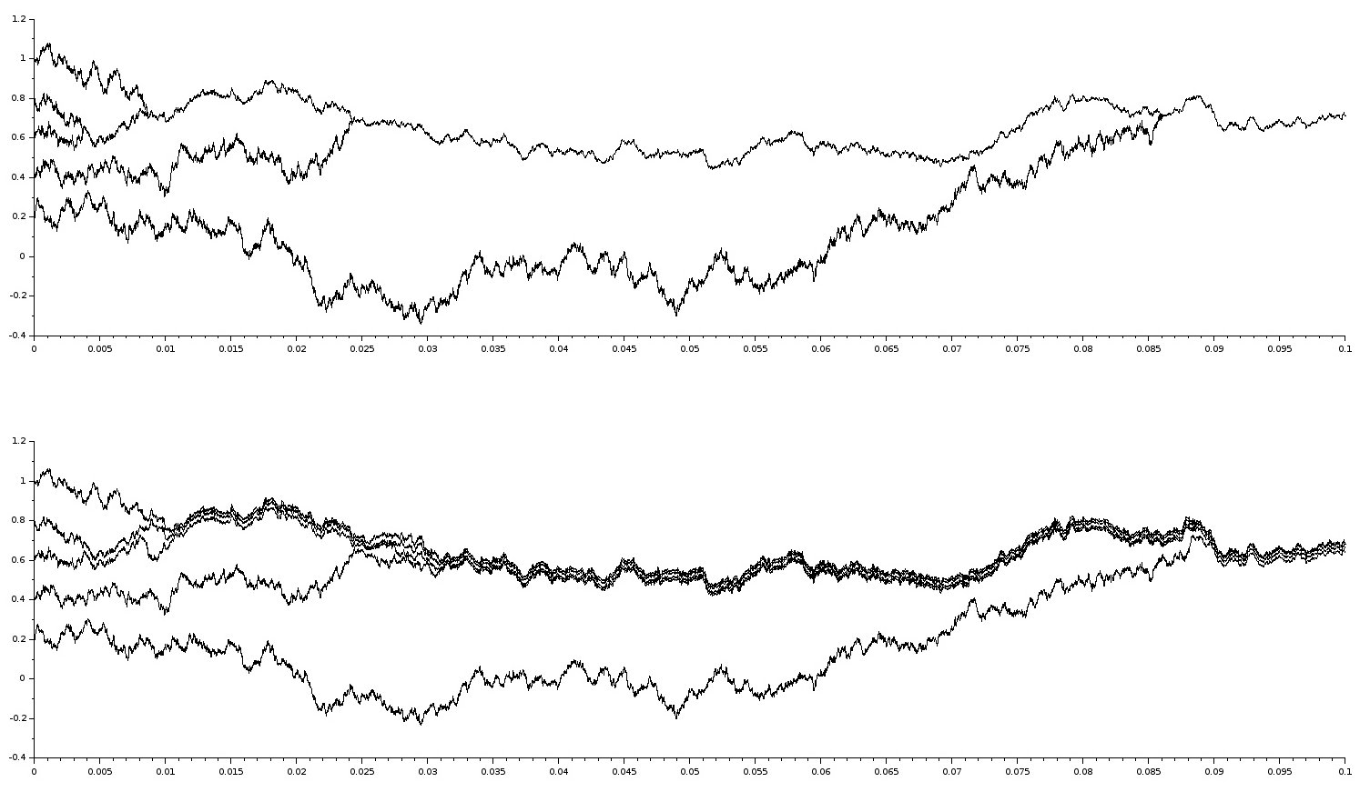
Refer to caption
Figure 1: Two simulations, based on the same underlying Brownian sheet, for the limit process (μt)t∈[0,T](\mu_{t})_{t\in[0,T]} (on top) and for the process (μtσ,ε)t∈[0,T](\mu_{t}^{\sigma,\varepsilon})_{t\in[0,T]} with positive σ\sigma and ε\varepsilon (on bottom). The horizontal axis represents time. On the vertical axis, we put the position of the particles (initially, we took five particles on [0,1][0,1]).

It is interesting to wonder how the coalescence property of the process yy translates to its smooth approximation yσ,εy_{\sigma,\varepsilon}: two paths (yσ,ε​(u,t))t∈[0,T](y_{\sigma,\varepsilon}(u,t))_{t\in[0,T]} and (yσ,ε​(v,t))t∈[0,T](y_{\sigma,\varepsilon}(v,t))_{t\in[0,T]}, starting from two distinct points g⁡(u)g(u) and g⁡(v)g(v), do not meet, which means that yσ,ε​(⋅,t)y_{\sigma,\varepsilon}(\cdot,t) is non-decreasing for each fixed tt. If yσ,ε​(u,⋅)y_{\sigma,\varepsilon}(u,\cdot) and yσ,ε​(v,⋅)y_{\sigma,\varepsilon}(v,\cdot) get close enough, at distance smaller than σ\sigma, they begin to interact and to move together, whereas as long as they remain at distance greater than σ\sigma, they move "independently": more precisely, the covariation ⟨yσ,ε​(u,⋅),yσ,ε​(v,⋅)⟩t\langle y_{\sigma,\varepsilon}(u,\cdot),y_{\sigma,\varepsilon}(v,\cdot)\rangle_{t} is equal to zero for every time t⩽τu,vσ:=inf{s⩾0:|yσ,ε​(u,s)−yσ,ε​(v,s)|⩽σ}t\leqslant\tau^{\sigma}_{u,v}:=\inf\{s\geqslant 0:|y_{\sigma,\varepsilon}(u,s)-y_{\sigma,\varepsilon}(v,s)|\leqslant\sigma\} (see figure 1).

Organisation of the article

We begin in Section 2 by proving Theorem 1.1, which states that a process yy satisfying properties (i)(i)-(i​v)(iv) admits a representation in terms of a Brownian sheet. In Section 3, given a two-dimensional Brownian sheet, we prove the existence of a smooth process in the space L2​([0,1],𝒞⁡[0,T])L_{2}([0,1],\mathcal{C}[0,T]) intended to approach Konarovskyi’s process of coalescing particles. This smooth process can be seen as a cloud of point-particles interacting with all the particles at a distance smaller than σ\sigma, and in which two particles have independent trajectories conditionally to the fact that the distance between them is greater than σ\sigma. When the distance becomes smaller than σ\sigma, both trajectories are correlated, mimicking the coalescence property.

Section 4 is devoted to the proof of convergence when the parameter ε\varepsilon and the range of interaction σ\sigma tend to zero, using a tightness criterion in L2​([0,1],𝒞⁡[0,T])L_{2}([0,1],\mathcal{C}[0,T]). In Section 5, we study the stochastic properties of the limit process, including the convergence of the mass process. The aim of this final part is to prove that the limit process yy satisfies properties (C​1)(C1)-(C​5)(C5) of Theorem 1.4, in other words that our sequence of short-range interaction processes converges in distribution to the process of coalescing particles.

In Appendix A, we give an Itô formula in the Wasserstein space for the limit process yy, after having recalled some basic definitions and properties of Lions’ differential calculus on 𝒫2​(ℝ)\mathcal{P}_{2}(\mathds{R}).

2 Singular representation of the process yy

Let (Ω,ℱ,ℙ)(\Omega,\mathcal{F},\mathbb{P}) be a probability space. Let us consider on (Ω,ℱ,ℙ)(\Omega,\mathcal{F},\mathbb{P}) a random process y∈L2​((0,1),𝒞⁡[0,T])y\in L_{2}((0,1),\mathcal{C}[0,T]) satisfying properties (i)(i)-(i​v)(iv). We refer to [11] for a comprehensive construction of yy. We will give another one later in this paper.

The aim of this Paragraph is to prove Theorem 1.1. Before that, we recall the definition of a Brownian sheet given by Walsh in [23, p.269]. Let (E,ℰ,ν)(E,\mathcal{E},\nu) be a Euclidean space equipped with Lebesgue measure. A white noise based on ν\nu is a random set function WW on the sets A∈ℰA\in\mathcal{E} of finite ν\nu-measure such that

  • •

    W⁡(A)W(A) is a 𝒩⁡(0,ν⁡(A))\mathcal{N}(0,\nu(A)) random variable,

  • •

    if A∩B=∅A\cap B=\emptyset, then W⁡(A)W(A) and W⁡(B)W(B) are independent and W⁡(A∩B)=W⁡(A)+W⁡(B)W(A\cap B)=W(A)+W(B).

Let T>0T>0. Consider E=[0,1]×[0,T]E=[0,1]\times[0,T] and ν\nu the associated Lebesgue measure. The Brownian sheet ww on [0,1]×[0,T][0,1]\times[0,T] associated to the white noise WW is the process (w⁡(u,t))u∈[0,1]×[0,T](w(u,t))_{u\in[0,1]\times[0,T]} defined by w⁡(u,t):=W⁡((0,u]×(0,t])w(u,t):=W((0,u]\times(0,t]).

Define the filtration (𝒢t)t∈[0,T](\mathcal{G}_{t})_{t\in[0,T]} by 𝒢t:=σ⁡(w⁡(u,s),u∈[0,1],s⩽t)\mathcal{G}_{t}:=\sigma(w(u,s),u\in[0,1],s\leqslant t). Then in particular,

  • (i)

    for each (𝒢t)t∈[0,T](\mathcal{G}_{t})_{t\in[0,T]}-progressively measurable function ff defined on [0,1]×[0,T][0,1]\times[0,T] such that ∫0T∫01f2​(u,s)​𝑑u​𝑑s<+∞\int_{0}^{T}\int_{0}^{1}f^{2}(u,s)\mathrm{d}u\mathrm{d}s<+\infty almost surely, the process (∫0t∫01f⁡(u,s)​𝑑w​(u,s))t∈[0,T]\left(\int_{0}^{t}\int_{0}^{1}f(u,s)\mathrm{d}w(u,s)\right)_{t\in[0,T]} is a local martingale (we often write d​w​(u,s)\mathrm{d}w(u,s) instead of w⁡(d​u,d​s)w(\mathrm{d}u,\mathrm{d}s));

  • (ii)

    for each f1f_{1} and f2f_{2} satisfying the same conditions as ff,

    ⟨∫0⋅∫01f1​(u,s)​𝑑w​(u,s),∫0⋅∫01f2​(u,s)​𝑑w​(u,s)⟩t\displaystyle\langle\int_{0}^{\cdot}\!\!\int_{0}^{1}f_{1}(u,s)\mathrm{d}w(u,s),\int_{0}^{\cdot}\!\!\int_{0}^{1}f_{2}(u,s)\mathrm{d}w(u,s)\rangle_{t} =∫0t∫01f1​(u,s)​f2​(u,s)​𝑑u​𝑑s.\displaystyle=\int_{0}^{t}\!\!\int_{0}^{1}f_{1}(u,s)f_{2}(u,s)\mathrm{d}u\mathrm{d}s.

By Lévy’s characterization of the Brownian motion, a process ww satisfying (i)(i) and (i​i)(ii) is a Brownian sheet. Let us now prove Theorem 1.1.

Proof (Theorem 1.1).

We take a Brownian sheet η\eta on [0,1]×[0,T][0,1]\times[0,T] independent of the process yy, constructed by possibly extending the probability space (Ω,ℱ,ℙ)(\Omega,\mathcal{F},\mathbb{P}). Then, we define (w⁡(u,t))u∈[0,1],t∈[0,T](w(u,t))_{u\in[0,1],t\in[0,T]} by w⁡(0,⋅)≡0w(0,\cdot)\equiv 0, w⁡(⋅,0)≡0w(\cdot,0)\equiv 0 and:

w(du,dt)=η(du,dt)+y(u,dt)du−1m⁡(u,t)∫01𝟙{y(u,t)=y(u′,t)}η(du′,dt)du.w(\mathrm{d}u,\mathrm{d}t)=\eta(\mathrm{d}u,\mathrm{d}t)+y(u,\mathrm{d}t)\mathrm{d}u-\frac{1}{m(u,t)}\int_{0}^{1}\mathds{1}_{\{y(u,t)=y(u^{\prime},t)\}}\eta(\mathrm{d}u^{\prime},\mathrm{d}t)\mathrm{d}u.

We denote by ℋt\mathcal{H}_{t} the filtration σ⁡((y⁡(u,s))u∈[0,1],s⩽t,(η⁡(u,s))u∈[0,1],s⩽t)\sigma((y(u,s))_{u\in[0,1],s\leqslant t},(\eta(u,s))_{u\in[0,1],s\leqslant t}).

In order to prove that ww is an (ℋt)t∈[0,T](\mathcal{H}_{t})_{t\in[0,T]}-Brownian sheet on [0,1]×[0,T][0,1]\times[0,T], let us consider two (ℋt)t∈[0,T](\mathcal{H}_{t})_{t\in[0,T]}-progressively measurable functions f1f_{1} and f2f_{2} and compute, using independence of η\eta and yy:

⟨∫0⋅∫01f1​(u,s)​𝑑w​(u,s),∫0⋅∫01f2​(v,s)​𝑑w​(v,s)⟩t=V1+V2−V3−V4+V5,\langle\int_{0}^{\cdot}\!\!\int_{0}^{1}f_{1}(u,s)\mathrm{d}w(u,s),\int_{0}^{\cdot}\!\!\int_{0}^{1}f_{2}(v,s)\mathrm{d}w(v,s)\rangle_{t}=V_{1}+V_{2}-V_{3}-V_{4}+V_{5},

where

V1:=⟨∫0⋅∫01f1​(u,s)​𝑑η​(u,s),∫0⋅∫01f2​(v,s)​𝑑η​(v,s)⟩t=∫0t∫01f1​(u,s)​f2​(u,s)​𝑑u​𝑑s,V_{1}:=\langle\int_{0}^{\cdot}\!\!\int_{0}^{1}f_{1}(u,s)\mathrm{d}\eta(u,s),\int_{0}^{\cdot}\!\!\int_{0}^{1}f_{2}(v,s)\mathrm{d}\eta(v,s)\rangle_{t}=\int_{0}^{t}\!\!\int_{0}^{1}f_{1}(u,s)f_{2}(u,s)\mathrm{d}u\mathrm{d}s,

since η\eta is an (ℋt)t∈[0,T](\mathcal{H}_{t})_{t\in[0,T]}-Brownian sheet;

V2\displaystyle V_{2} :=⟨∫0⋅∫01f1​(u,s)​𝑑y​(u,s)​𝑑u,∫0⋅∫01f2​(v,s)​𝑑y​(v,s)​𝑑v⟩t\displaystyle:=\langle\int_{0}^{\cdot}\!\!\int_{0}^{1}f_{1}(u,s)\mathrm{d}y(u,s)\mathrm{d}u,\int_{0}^{\cdot}\!\!\int_{0}^{1}f_{2}(v,s)\mathrm{d}y(v,s)\mathrm{d}v\rangle_{t}
=∫0t∫01∫01f1​(u,s)​f2​(v,s)​𝟙{y(u,s)=y(v,s)}m⁡(u,s)​𝑑u​𝑑v​𝑑s,\displaystyle=\int_{0}^{t}\!\!\int_{0}^{1}\!\!\int_{0}^{1}f_{1}(u,s)f_{2}(v,s)\frac{\mathds{1}_{\{y(u,s)=y(v,s)\}}}{m(u,s)}\mathrm{d}u\mathrm{d}v\mathrm{d}s,

using property (i​v)(iv) of process yy;

V3\displaystyle V_{3} :=⟨∫0⋅∫01f1(u,s)dη(u,s),∫0⋅∫01f2​(v,s)m⁡(v,s)∫01𝟙{y(v,s)=y(v′,s)}dη(v′,s)dv⟩t\displaystyle:=\langle\int_{0}^{\cdot}\!\!\int_{0}^{1}f_{1}(u,s)\mathrm{d}\eta(u,s),\int_{0}^{\cdot}\!\!\int_{0}^{1}\frac{f_{2}(v,s)}{m(v,s)}\int_{0}^{1}\mathds{1}_{\{y(v,s)=y(v^{\prime},s)\}}\mathrm{d}\eta(v^{\prime},s)\mathrm{d}v\rangle_{t}
=∫0t∫01∫01f1​(u,s)​f2​(v,s)m⁡(v,s)𝟙{y(v,s)=y(u,s)}dudvds=V2,\displaystyle=\int_{0}^{t}\!\!\int_{0}^{1}\!\!\int_{0}^{1}\frac{f_{1}(u,s)f_{2}(v,s)}{m(v,s)}\mathds{1}_{\{y(v,s)=y(u,s)\}}\mathrm{d}u\mathrm{d}v\mathrm{d}s=V_{2},

since m⁡(u,s)=m⁡(v,s)m(u,s)=m(v,s) whenever y⁡(u,s)y(u,s) is equal to y⁡(v,s)y(v,s). By similar computations,

V4:=⟨∫0⋅∫01f1​(u,s)m⁡(u,s)∫01𝟙{y(u,s)=y(u′,s)}dη(u′,s)du,∫0⋅∫01f2(v,s)dη(v,s)⟩t=V2,V_{4}:=\langle\int_{0}^{\cdot}\!\!\int_{0}^{1}\frac{f_{1}(u,s)}{m(u,s)}\int_{0}^{1}\mathds{1}_{\{y(u,s)=y(u^{\prime},s)\}}\mathrm{d}\eta(u^{\prime},s)\mathrm{d}u,\int_{0}^{\cdot}\!\!\int_{0}^{1}f_{2}(v,s)\mathrm{d}\eta(v,s)\rangle_{t}=V_{2},

and

V5:\displaystyle V_{5}: =⟨∫0⋅∫01f1​(u,s)m⁡(u,s)∫01𝟙{y(u,s)=y(u′,s)}dη(u′,s)du,∫0⋅∫01f2​(v,s)m⁡(v,s)∫01𝟙{y(v,s)=y(v′,s)}dη(v′,s)dv⟩t\displaystyle=\langle\int\limits_{0}^{\cdot}\int\limits_{0}^{1}\frac{f_{1}(u,s)}{m(u,s)}\int\limits_{0}^{1}\mathds{1}_{\{y(u,s)=y(u^{\prime},s)\}}\mathrm{d}\eta(u^{\prime},s)\mathrm{d}u,\int\limits_{0}^{\cdot}\int\limits_{0}^{1}\frac{f_{2}(v,s)}{m(v,s)}\int\limits_{0}^{1}\mathds{1}_{\{y(v,s)=y(v^{\prime},s)\}}\mathrm{d}\eta(v^{\prime},s)\mathrm{d}v\rangle_{t}
=∫0t∫01∫01∫01f1​(u,s)​f2​(v,s)m⁡(u,s)​m​(v,s)𝟙{y(u,s)=y(u′,s)}𝟙{y(v,s)=y(u′,s)}du′dudvds\displaystyle=\int_{0}^{t}\!\!\int_{0}^{1}\!\!\int_{0}^{1}\!\!\int_{0}^{1}\frac{f_{1}(u,s)f_{2}(v,s)}{m(u,s)m(v,s)}\mathds{1}_{\{y(u,s)=y(u^{\prime},s)\}}\mathds{1}_{\{y(v,s)=y(u^{\prime},s)\}}\mathrm{d}u^{\prime}\mathrm{d}u\mathrm{d}v\mathrm{d}s
=∫0t∫01∫01f1​(u,s)​f2​(v,s)m​(u,s)2(∫01𝟙{y(u,s)=y(u′,s)}du′)𝟙{y(u,s)=y(v,s)}dudvds\displaystyle=\int_{0}^{t}\!\!\int_{0}^{1}\!\!\int_{0}^{1}\frac{f_{1}(u,s)f_{2}(v,s)}{m(u,s)^{2}}\left(\int_{0}^{1}\mathds{1}_{\{y(u,s)=y(u^{\prime},s)\}}\mathrm{d}u^{\prime}\right)\mathds{1}_{\{y(u,s)=y(v,s)\}}\mathrm{d}u\mathrm{d}v\mathrm{d}s
=∫0t∫01∫01f1​(u,s)​f2​(v,s)m⁡(u,s)𝟙{y(u,s)=y(v,s)}dudvds=V2.\displaystyle=\int_{0}^{t}\!\!\int_{0}^{1}\!\!\int_{0}^{1}\frac{f_{1}(u,s)f_{2}(v,s)}{m(u,s)}\mathds{1}_{\{y(u,s)=y(v,s)\}}\mathrm{d}u\mathrm{d}v\mathrm{d}s=V_{2}.

To sum up,

⟨∫0⋅∫01f1​(u,s)​𝑑w​(u,s),∫0⋅∫01f2​(v,s)​𝑑w​(v,s)⟩t=V1=∫0t∫01f1​(u,s)​f2​(u,s)​𝑑u​𝑑s,\langle\int_{0}^{\cdot}\!\!\int_{0}^{1}f_{1}(u,s)\mathrm{d}w(u,s),\int_{0}^{\cdot}\!\!\int_{0}^{1}f_{2}(v,s)\mathrm{d}w(v,s)\rangle_{t}=V_{1}=\int_{0}^{t}\!\!\int_{0}^{1}f_{1}(u,s)f_{2}(u,s)\mathrm{d}u\mathrm{d}s,

whence ww is an (ℋt)t∈[0,T](\mathcal{H}_{t})_{t\in[0,T]}-Brownian sheet. Finally, we show that (y,w)(y,w) satisfies equation (1):

∫0t∫01𝟙{y(u,s)=y(u′,s)}m⁡(u,s)​𝑑w​(u′,s)\displaystyle\int_{0}^{t}\!\!\int_{0}^{1}\frac{\mathds{1}_{\{y(u,s)=y(u^{\prime},s)\}}}{m(u,s)}\mathrm{d}w(u^{\prime},s) =∫0t∫01𝟙{y(u,s)=y(u′,s)}m⁡(u,s)​𝑑η​(u′,s)\displaystyle=\int_{0}^{t}\!\!\int_{0}^{1}\frac{\mathds{1}_{\{y(u,s)=y(u^{\prime},s)\}}}{m(u,s)}\mathrm{d}\eta(u^{\prime},s) (=:W1=:W_{1})
+∫0t∫01𝟙{y(u,s)=y(u′,s)}m⁡(u,s)dy(u′,s)du′\displaystyle+\int_{0}^{t}\!\!\int_{0}^{1}\frac{\mathds{1}_{\{y(u,s)=y(u^{\prime},s)\}}}{m(u,s)}\mathrm{d}y(u^{\prime},s)\mathrm{d}u^{\prime} (=:W2=:W_{2})
−∫0t∫01𝟙{y(u,s)=y(u′,s)}m⁡(u,s)∫01𝟙{y(u′,s)=y(v,s)}m⁡(u′,s)dη(v,s)du′.\displaystyle-\int_{0}^{t}\!\!\int_{0}^{1}\frac{\mathds{1}_{\{y(u,s)=y(u^{\prime},s)\}}}{m(u,s)}\int_{0}^{1}\frac{\mathds{1}_{\{y(u^{\prime},s)=y(v,s)\}}}{m(u^{\prime},s)}\mathrm{d}\eta(v,s)\mathrm{d}u^{\prime}. (=:W3=:W_{3})

The result follows from the two below equalities:

W2=∫0t∫01𝟙{y(u,s)=y(u′,s)}m⁡(u,s)​𝑑y​(u,s)​d​u′=∫0td​y​(u,s)=y⁡(u,t)−y⁡(u,0)=y⁡(u,t)−g⁡(u);W_{2}=\int_{0}^{t}\!\!\int_{0}^{1}\frac{\mathds{1}_{\{y(u,s)=y(u^{\prime},s)\}}}{m(u,s)}\mathrm{d}y(u,s)\mathrm{d}u^{\prime}=\int_{0}^{t}\mathrm{d}y(u,s)=y(u,t)-y(u,0)=y(u,t)-g(u);
W3\displaystyle W_{3} =∫0t∫01𝟙{y(u,s)=y(u′,s)}m⁡(u,s)​∫01𝟙{y(u′,s)=y(v,s)}m⁡(v,s)​𝑑η​(v,s)​d​u′\displaystyle=\int_{0}^{t}\!\!\int_{0}^{1}\frac{\mathds{1}_{\{y(u,s)=y(u^{\prime},s)\}}}{m(u,s)}\int_{0}^{1}\frac{\mathds{1}_{\{y(u^{\prime},s)=y(v,s)\}}}{m(v,s)}\mathrm{d}\eta(v,s)\mathrm{d}u^{\prime}
=∫0t∫01𝟙{y(u,s)=y(v,s)}m⁡(u,s)​m​(v,s)(∫01𝟙{y(u′,s)=y(v,s)}du′)dη(v,s)=∫0t∫01𝟙{y(u,s)=y(v,s)}m⁡(u,s)dη(v,s),\displaystyle=\int_{0}^{t}\!\!\int_{0}^{1}\frac{\mathds{1}_{\{y(u,s)=y(v,s)\}}}{m(u,s)m(v,s)}\left(\int_{0}^{1}\mathds{1}_{\{y(u^{\prime},s)=y(v,s)\}}\mathrm{d}u^{\prime}\right)\mathrm{d}\eta(v,s)=\int_{0}^{t}\!\!\int_{0}^{1}\frac{\mathds{1}_{\{y(u,s)=y(v,s)\}}}{m(u,s)}\mathrm{d}\eta(v,s),

which implies that W3=W1W_{3}=W_{1} and consequently equation (1). ∎

Therefore, every solution of the martingale problem (i)(i)-(i​v)(iv) has a representation in terms of a Brownian sheet. In the next Section, we will construct, given a Brownian sheet, an approximation of the process yy.

3 Construction of a process with short-range interactions

Let (Ω,ℱ,ℙ)(\Omega,\mathcal{F},\mathbb{P}) be a probability space, on which we define a Brownian sheet ww on [0,1]×[0,T][0,1]\times[0,T]. We associate to that process the filtration 𝒢t:=σ⁡(w⁡(u,s),u∈[0,1],s⩽t)\mathcal{G}_{t}:=\sigma(w(u,s),u\in[0,1],s\leqslant t). Up to completing the filtration, we assume that 𝒢0\mathcal{G}_{0} contains all the ℙ\mathbb{P}-null sets of ℱ\mathcal{F} and that the filtration (𝒢t)t∈[0,T](\mathcal{G}_{t})_{t\in[0,T]} is right-continuous.

Fix σ>0\sigma>0 and ε>0\varepsilon>0. Let φσ\varphi_{\sigma} denote a smooth and even function, bounded by 1, equal to 1 on [0,σ3][0,\frac{\sigma}{3}] and equal to 0 on [σ2,+∞)[\frac{\sigma}{2},+\infty). Recall that ℒ2+↑​[0,1]\mathcal{L}^{\uparrow}_{2+}[0,1] represents the set of non-decreasing and càdlàg functions g:[0,1]→ℝg:[0,1]\rightarrow\mathds{R} such that there exists p>2p>2 satisfying ∫01|g⁡(u)|p​𝑑u<+∞\int_{0}^{1}|g(u)|^{p}\mathrm{d}u<+\infty. The aim of this Section is to construct, for each initial quantile function g∈ℒ2+↑​[0,1]g\in\mathcal{L}^{\uparrow}_{2+}[0,1], a square integrable random variable yσ,εgy^{g}_{\sigma,\varepsilon} taking values in L2​([0,1],𝒞⁡[0,T])L_{2}([0,1],\mathcal{C}[0,T]) such that almost surely, for every t∈[0,T]t\in[0,T], the following equality holds in L2​[0,1]L_{2}[0,1]:

yσ,εg​(⋅,t)=g+∫0t∫01φσ​(yσ,εg​(⋅,s)−yσ,εg​(u′,s))ε+∫01φσ2​(yσ,εg​(⋅,s)−yσ,εg​(v,s))​𝑑v​𝑑w​(u′,s).y^{g}_{\sigma,\varepsilon}(\cdot,t)=g+\int_{0}^{t}\!\!\int_{0}^{1}\frac{\mathds{\varphi}_{\sigma}(y^{g}_{\sigma,\varepsilon}(\cdot,s)-y^{g}_{\sigma,\varepsilon}(u^{\prime},s))}{\varepsilon+\int_{0}^{1}\varphi_{\sigma}^{2}(y^{g}_{\sigma,\varepsilon}(\cdot,s)-y^{g}_{\sigma,\varepsilon}(v,s))\mathrm{d}v}\mathrm{d}w(u^{\prime},s). (3)
Remark 3.1.

We add the parameter ε\varepsilon to the denominator in order to ensure that it is bounded by below. We also point out that relation (3) has to be compared with equation (1), where x↦𝟙{x=0}x\mapsto\mathds{1}_{\{x=0\}} is replaced by the function φσ\varphi_{\sigma}.

More precisely, we will prove the following Proposition. Recall that L2↑​[0,1]L^{\uparrow}_{2}[0,1] represents the set of functions f∈L2​[0,1]f\in L_{2}[0,1] such that there is a non-decreasing and càdlàg element in the equivalence class of ff.

Proposition 3.2.

Let g∈ℒ2+↑​[0,1]g\in\mathcal{L}^{\uparrow}_{2+}[0,1]. There exists an L2↑​[0,1]L^{\uparrow}_{2}[0,1]-valued process (Yσ,εg​(t))t∈[0,T]=(yσ,εg​(⋅,t))t∈[0,T](Y^{g}_{\sigma,\varepsilon}(t))_{t\in[0,T]}=(y^{g}_{\sigma,\varepsilon}(\cdot,t))_{t\in[0,T]} such that:

  • (A​1)(A1)

    Yσ,εg​(0)=gY^{g}_{\sigma,\varepsilon}(0)=g;

  • (A​2)(A2)

    Yσ,εgY^{g}_{\sigma,\varepsilon} is a square integrable continuous L2↑​[0,1]L^{\uparrow}_{2}[0,1]-valued (ℱtσ,ε)t∈[0,T](\mathcal{F}^{\sigma,\varepsilon}_{t})_{t\in[0,T]}-martingale, where ℱtσ,ε:=σ⁡(Yσ,εg​(s),s⩽t)\mathcal{F}^{\sigma,\varepsilon}_{t}:=\sigma(Y^{g}_{\sigma,\varepsilon}(s),s\leqslant t);

  • (A​3)(A3)

    for every h,k∈L2​[0,1]h,k\in L_{2}[0,1],

    ⟨(Yσ,εg,h)L2,(Yσ,εg,k)L2⟩t=∫0t∫01∫01h⁡(u)​k​(u′)​mσ,εg​(u,u′,s)(ε+mσ,εg​(u,s))​(ε+mσ,εg​(u′,s))​𝑑u​d​u′​𝑑s,\displaystyle\langle(Y^{g}_{\sigma,\varepsilon},h)_{L_{2}},(Y^{g}_{\sigma,\varepsilon},k)_{L_{2}}\rangle_{t}=\int_{0}^{t}\!\!\int_{0}^{1}\!\!\int_{0}^{1}h(u)k(u^{\prime})\frac{m^{g}_{\sigma,\varepsilon}(u,u^{\prime},s)}{(\varepsilon+m^{g}_{\sigma,\varepsilon}(u,s))(\varepsilon+m^{g}_{\sigma,\varepsilon}(u^{\prime},s))}\mathrm{d}u\mathrm{d}u^{\prime}\mathrm{d}s,

    where mσ,εg​(u,u′,s)=∫01φσ​(yσ,εg​(u,s)−yσ,εg​(v,s))​φσ​(yσ,εg​(u′,s)−yσ,εg​(v,s))​𝑑vm^{g}_{\sigma,\varepsilon}(u,u^{\prime},s)=\int_{0}^{1}\varphi_{\sigma}(y^{g}_{\sigma,\varepsilon}(u,s)-y^{g}_{\sigma,\varepsilon}(v,s))\varphi_{\sigma}(y^{g}_{\sigma,\varepsilon}(u^{\prime},s)-y^{g}_{\sigma,\varepsilon}(v,s))\mathrm{d}v and
    mσ,εg​(u,s)=∫01φσ2​(yσ,εg​(u,s)−yσ,εg​(v,s))​𝑑vm^{g}_{\sigma,\varepsilon}(u,s)=\int_{0}^{1}\varphi_{\sigma}^{2}(y^{g}_{\sigma,\varepsilon}(u,s)-y^{g}_{\sigma,\varepsilon}(v,s))\mathrm{d}v.

3.1 Existence of an approximate solution

Denote by ℳ\mathcal{M} the set of random variables z∈L2​(Ω,𝒞⁡([0,T],L2​(0,1)))z\in L_{2}(\Omega,\mathcal{C}([0,T],L_{2}(0,1))) such that (z⁡(ω,⋅,t))t∈[0,T](z(\omega,\cdot,t))_{t\in[0,T]} is a (𝒢t)t∈[0,T](\mathcal{G}_{t})_{t\in[0,T]}-progressively measurable process with values in L2​(0,1)L_{2}(0,1). We consider the following norm on ℳ\mathcal{M}:

‖z‖ℳ=𝔼​[supt⩽T∫01|z⁡(u,t)|2​𝑑u]1/2.\|z\|_{\mathcal{M}}=\mathbb{E}\left[\sup_{t\leqslant T}\int_{0}^{1}|z(u,t)|^{2}\mathrm{d}u\right]^{1/2}.

Throughout this Section, σ\sigma and ε\varepsilon are two fixed positive numbers. To begin, we want to prove that the map ψ:ℳ→ℳ\psi:\mathcal{M}\rightarrow\mathcal{M}, defined below, admits a unique fixed point. Fix g∈ℒ2+↑​[0,1]g\in\mathcal{L}^{\uparrow}_{2+}[0,1] an initial quantile function. For all z∈ℳz\in\mathcal{M}, define:

ψ⁡(z)​(ω,u,t):=g⁡(u)+∫0t∫01φσ​(z⁡(ω,u,s)−z⁡(ω,u′,s))ε+mσ​(ω,u,s)​𝑑w​(ω,u′,s),\psi(z)(\omega,u,t):=g(u)+\int_{0}^{t}\!\!\int_{0}^{1}\frac{\varphi_{\sigma}(z(\omega,u,s)-z(\omega,u^{\prime},s))}{\varepsilon+m_{\sigma}(\omega,u,s)}\mathrm{d}w(\omega,u^{\prime},s), (4)

where mσ​(ω,u,s)=∫01φσ2​(z⁡(ω,u,s)−z⁡(ω,v,s))​𝑑vm_{\sigma}(\omega,u,s)=\int_{0}^{1}\varphi_{\sigma}^{2}(z(\omega,u,s)-z(\omega,v,s))\mathrm{d}v. We start by making sure that ψ\psi is well-defined.

Proposition 3.3.

For all z∈ℳz\in\mathcal{M}, ψ⁡(z)\psi(z) belongs to ℳ\mathcal{M}. Furthermore, (ψ⁡(z)​(⋅,t))t∈[0,T](\psi(z)(\cdot,t))_{t\in[0,T]} is an L2​(0,1)L_{2}(0,1)-valued continuous (𝒢t)t∈[0,T](\mathcal{G}_{t})_{t\in[0,T]}-martingale.

Remark 3.4.

The definition of an L2↑​[0,1]L^{\uparrow}_{2}[0,1]-valued martingale was given in Definition 1.3. Up to replacing L2↑L^{\uparrow}_{2} by L2L_{2}, the definition of an L2​(0,1)L_{2}(0,1)-valued martingale is exactly the same.

Proof.

We want to prove that (ψ⁡(z)​(⋅,t))t∈[0,T](\psi(z)(\cdot,t))_{t\in[0,T]} is an L2​(0,1)L_{2}(0,1)-valued (𝒢t)t∈[0,T](\mathcal{G}_{t})_{t\in[0,T]}-martingale. Since zz belongs to ℳ\mathcal{M}, the process (z⁡(⋅,t))t∈[0,T](z(\cdot,t))_{t\in[0,T]} is (𝒢t)t∈[0,T](\mathcal{G}_{t})_{t\in[0,T]}-progressively measurable. Therefore (mσ​(⋅,t))t∈[0,T](m_{\sigma}(\cdot,t))_{t\in[0,T]} is also (𝒢t)t∈[0,T](\mathcal{G}_{t})_{t\in[0,T]}-progressively measurable and we deduce that (ψ⁡(z)​(⋅,t))t∈[0,T](\psi(z)(\cdot,t))_{t\in[0,T]} is (𝒢t)t∈[0,T](\mathcal{G}_{t})_{t\in[0,T]}-progressively measurable.

Then, we check that for each t∈[0,T]t\in[0,T], ψ⁡(z)​(⋅,t)∈L2​(0,1)\psi(z)(\cdot,t)\in L_{2}(0,1) and 𝔼⁡[‖ψ⁡(z)​(⋅,t)‖L2]<∞\mathbb{E}\left[\|\psi(z)(\cdot,t)\|_{L_{2}}\right]<\infty. We deduce this statement by recalling that ‖g‖L2<+∞\|g\|_{L_{2}}<+\infty, because g∈ℒ2+↑​[0,1]g\in\mathcal{L}^{\uparrow}_{2+}[0,1], and by computing:

𝔼​[‖∫0t∫01φσ​(z⁡(⋅,s)−z⁡(u′,s))ε+mσ​(⋅,s)​dw​(u′,s)‖L2]2⩽𝔼⁡[‖∫0t∫01φσ​(z⁡(⋅,s)−z⁡(u′,s))ε+mσ​(⋅,s)​dw​(u′,s)‖L22]=𝔼⁡[∫01|∫0t∫01φσ​(z⁡(u,s)−z⁡(u′,s))ε+mσ​(u,s)​dw​(u′,s)|2​du]=∫01𝔼⁡[|∫0t∫01φσ​(z⁡(u,s)−z⁡(u′,s))ε+mσ​(u,s)​𝑑w​(u′,s)|2]​𝑑u=∫01𝔼⁡[∫0t∫01(φσ​(z⁡(u,s)−z⁡(u′,s))ε+mσ​(u,s))2​d​u′​𝑑s]​𝑑u⩽‖φσ‖∞2​tε2=tε2<+∞.\mathbb{E}\left[\left\|\int_{0}^{t}\!\!\int_{0}^{1}\frac{\varphi_{\sigma}(z(\cdot,s)-z(u^{\prime},s))}{\varepsilon+m_{\sigma}(\cdot,s)}\mathrm{d}w(u^{\prime},s)\right\|_{L_{2}}\right]^{2}\!\!\leqslant\mathbb{E}\left[\left\|\int_{0}^{t}\!\!\int_{0}^{1}\frac{\varphi_{\sigma}(z(\cdot,s)-z(u^{\prime},s))}{\varepsilon+m_{\sigma}(\cdot,s)}\mathrm{d}w(u^{\prime},s)\right\|_{L_{2}}^{2}\right]\\ \begin{aligned} &=\mathbb{E}\left[\int_{0}^{1}\left|\int_{0}^{t}\!\!\int_{0}^{1}\frac{\varphi_{\sigma}(z(u,s)-z(u^{\prime},s))}{\varepsilon+m_{\sigma}(u,s)}\mathrm{d}w(u^{\prime},s)\right|^{2}\mathrm{d}u\right]\\ &=\int_{0}^{1}\mathbb{E}\left[\left|\int_{0}^{t}\!\!\int_{0}^{1}\frac{\varphi_{\sigma}(z(u,s)-z(u^{\prime},s))}{\varepsilon+m_{\sigma}(u,s)}\mathrm{d}w(u^{\prime},s)\right|^{2}\right]\mathrm{d}u\\ &=\int_{0}^{1}\mathbb{E}\left[\ \int_{0}^{t}\!\!\int_{0}^{1}\left(\frac{\varphi_{\sigma}(z(u,s)-z(u^{\prime},s))}{\varepsilon+m_{\sigma}(u,s)}\right)^{2}\mathrm{d}u^{\prime}\mathrm{d}s\right]\mathrm{d}u\\ &\leqslant\frac{\|\varphi_{\sigma}\|_{\infty}^{2}t}{\varepsilon^{2}}=\frac{t}{\varepsilon^{2}}<+\infty.\end{aligned} (5)

Furthermore, for each h∈L2​[0,1]h\in L_{2}[0,1],

(ψ⁡(z)​(⋅,t),h)L2=(g,h)L2+∫0t∫01∫01h⁡(u)​φσ​(z⁡(u,s)−z⁡(u′,s))ε+mσ​(u,s)​𝑑u​𝑑w​(u′,s)\displaystyle(\psi(z)(\cdot,t),h)_{L_{2}}=(g,h)_{L_{2}}+\int_{0}^{t}\!\!\int_{0}^{1}\!\!\int_{0}^{1}h(u)\frac{\varphi_{\sigma}(z(u,s)-z(u^{\prime},s))}{\varepsilon+m_{\sigma}(u,s)}\mathrm{d}u\mathrm{d}w(u^{\prime},s)

is a (𝒢t)t∈[0,T](\mathcal{G}_{t})_{t\in[0,T]}-local martingale. Then, we compute the quadratic variation:

𝔼⁡[⟨(ψ⁡(z),h)L2,(ψ⁡(z),h)L2⟩t]=∫0t∫01∫01∫01h⁡(u1)​h​(u2)​φσ​(z⁡(u1,s)−z⁡(u′,s))​φσ​(z⁡(u2,s)−z⁡(u′,s))(ε+mσ​(u1,s))​(ε+mσ​(u2,s))​d​u1​d​u2​d​u′​ds⩽tε2​‖h‖L22.\mathbb{E}\left[\langle(\psi(z),h)_{L_{2}},(\psi(z),h)_{L_{2}}\rangle_{t}\right]\\ =\!\!\int_{0}^{t}\!\!\int_{0}^{1}\!\!\int_{0}^{1}\!\!\int_{0}^{1}\!\!h(u_{1})h(u_{2})\frac{\varphi_{\sigma}(z(u_{1},s)-z(u^{\prime},s))\varphi_{\sigma}(z(u_{2},s)-z(u^{\prime},s))}{(\varepsilon+m_{\sigma}(u_{1},s))(\varepsilon+m_{\sigma}(u_{2},s))}\mathrm{d}u_{1}\mathrm{d}u_{2}\mathrm{d}u^{\prime}\mathrm{d}s\leqslant\frac{t}{\varepsilon^{2}}\|h\|_{L_{2}}^{2}.

Since it is finite, the local martingale is actually a martingale.

Moreover, by Doob’s inequality (see Theorem 2.2 in [9, p.22])

‖ψ⁡(z)‖ℳ\displaystyle\|\psi(z)\|_{\mathcal{M}} =𝔼​[supt⩽T∫01|ψ⁡(z)​(u,t)|2​𝑑u]1/2\displaystyle=\mathbb{E}\left[\sup_{t\leqslant T}\int_{0}^{1}|\psi(z)(u,t)|^{2}\mathrm{d}u\right]^{1/2}
⩽‖g‖L2+𝔼​[supt⩽T∫01|∫0t∫01φσ​(z⁡(u,s)−z⁡(u′,s))ε+mσ​(u,s)​𝑑w​(u′,s)|2​𝑑u]1/2\displaystyle\leqslant\|g\|_{L_{2}}+\mathbb{E}\left[\sup_{t\leqslant T}\int_{0}^{1}\left|\int_{0}^{t}\!\!\int_{0}^{1}\frac{\varphi_{\sigma}(z(u,s)-z(u^{\prime},s))}{\varepsilon+m_{\sigma}(u,s)}\mathrm{d}w(u^{\prime},s)\right|^{2}\mathrm{d}u\right]^{1/2}
⩽‖g‖L2+2​𝔼​[∫01|∫0T∫01φσ​(z⁡(u,s)−z⁡(u′,s))ε+mσ​(u,s)​𝑑w​(u′,s)|2​𝑑u]1/2.\displaystyle\leqslant\|g\|_{L_{2}}+2\mathbb{E}\left[\int_{0}^{1}\left|\int_{0}^{T}\!\!\int_{0}^{1}\frac{\varphi_{\sigma}(z(u,s)-z(u^{\prime},s))}{\varepsilon+m_{\sigma}(u,s)}\mathrm{d}w(u^{\prime},s)\right|^{2}\mathrm{d}u\right]^{1/2}.

The last term is finite by (5). Thus ‖ψ⁡(z)‖ℳ\|\psi(z)\|_{\mathcal{M}} is finite and ψ⁡(z)\psi(z) belongs to ℳ\mathcal{M}, which concludes the proof. ∎

Let us now prove that ψ\psi has a unique fixed point:

Proposition 3.5.

Let σ>0\sigma>0 and ε>0\varepsilon>0. Then the map ψ:ℳ→ℳ\psi:\mathcal{M}\rightarrow\mathcal{M} defined by (4) has a unique fixed point in ℳ\mathcal{M}, denoted by yσ,εgy_{\sigma,\varepsilon}^{g}.

Proof.

For all n∈ℕn\in\mathds{N}, denote by ψn\psi^{n} the nn-fold composition of ψ\psi, where ψ0\psi^{0} denotes the identity function of ℳ\mathcal{M}. We want to prove that ψn\psi^{n} is a contraction for nn large enough.

Let z1z_{1} and z2z_{2} be two elements of ℳ\mathcal{M}. We define

hn​(t):=𝔼⁡[sups⩽t∫01|ψn​(z1)​(u,s)−ψn​(z2)​(u,s)|2​𝑑u].h_{n}(t):=\mathbb{E}\left[\sup_{s\leqslant t}\int_{0}^{1}|\psi^{n}(z_{1})(u,s)-\psi^{n}(z_{2})(u,s)|^{2}\mathrm{d}u\right].

Let us remark that hn​(T)=‖ψn​(z1)−ψn​(z2)‖ℳ2h_{n}(T)=\|\psi^{n}(z_{1})-\psi^{n}(z_{2})\|^{2}_{\mathcal{M}} and recall that, by Proposition 3.3, (ψ⁡(z1)​(⋅,t)−ψ⁡(z2)​(⋅,t))t∈[0,T](\psi(z_{1})(\cdot,t)-\psi(z_{2})(\cdot,t))_{t\in[0,T]} is a (𝒢t)t∈[0,T](\mathcal{G}_{t})_{t\in[0,T]}-martingale. We denote by mσ,1m_{\sigma,1} and mσ,2m_{\sigma,2} the masses associated respectively to z1z_{1} and z2z_{2}. By Doob’s inequality, we have:

h1​(t)\displaystyle h_{1}(t) =𝔼⁡[sups⩽t∫01|ψ⁡(z1)​(u,s)−ψ⁡(z2)​(u,s)|2​𝑑u]\displaystyle=\mathbb{E}\left[\sup_{s\leqslant t}\int_{0}^{1}|\psi(z_{1})(u,s)-\psi(z_{2})(u,s)|^{2}\mathrm{d}u\right]
=𝔼⁡[sups⩽t∫01|∫0s∫01(φσ​(z1​(u,r)−z1​(u′,r))ε+mσ,1​(u,r)−φσ​(z2​(u,r)−z2​(u′,r))ε+mσ,2​(u,r))​𝑑w​(u′,r)|2​𝑑u]\displaystyle=\mathbb{E}\left[\sup_{s\leqslant t}\int_{0}^{1}\left|\int_{0}^{s}\!\!\int_{0}^{1}\left(\frac{\varphi_{\sigma}(z_{1}(u,r)-z_{1}(u^{\prime},r))}{\varepsilon+m_{\sigma,1}(u,r)}-\frac{\varphi_{\sigma}(z_{2}(u,r)-z_{2}(u^{\prime},r))}{\varepsilon+m_{\sigma,2}(u,r)}\right)\mathrm{d}w(u^{\prime},r)\right|^{2}\mathrm{d}u\right]
⩽4​𝔼​[∫01∫0t∫01|φσ​(z1​(u,s)−z1​(u′,s))ε+mσ,1​(u,s)−φσ​(z2​(u,s)−z2​(u′,s))ε+mσ,2​(u,s)|2​d​u′​𝑑s​𝑑u].\displaystyle\leqslant 4\mathbb{E}\left[\int_{0}^{1}\!\!\int_{0}^{t}\!\!\int_{0}^{1}\left|\frac{\varphi_{\sigma}(z_{1}(u,s)-z_{1}(u^{\prime},s))}{\varepsilon+m_{\sigma,1}(u,s)}-\frac{\varphi_{\sigma}(z_{2}(u,s)-z_{2}(u^{\prime},s))}{\varepsilon+m_{\sigma,2}(u,s)}\right|^{2}\mathrm{d}u^{\prime}\mathrm{d}s\mathrm{d}u\right].

Furthermore, we compute:

|φσ​(z1​(u,s)−z1​(u′,s))ε+mσ,1​(u,s)−φσ​(z2​(u,s)−z2​(u′,s))ε+mσ,2​(u,s)|2⩽2​(|φσ​(z1​(u,s)−z1​(u′,s))−φσ​(z2​(u,s)−z2​(u′,s))ε+mσ,1​(u,s)|2CLOSEOPEN+|φσ​(z2​(u,s)−z2​(u′,s))(ε+mσ,1​(u,s))​(ε+mσ,2​(u,s))​(mσ,1​(u,s)−mσ,2​(u,s))|2).\left|\frac{\varphi_{\sigma}(z_{1}(u,s)-z_{1}(u^{\prime},s))}{\varepsilon+m_{\sigma,1}(u,s)}-\frac{\varphi_{\sigma}(z_{2}(u,s)-z_{2}(u^{\prime},s))}{\varepsilon+m_{\sigma,2}(u,s)}\right|^{2}\\ \leqslant 2\bigg(\left|\frac{\varphi_{\sigma}(z_{1}(u,s)-z_{1}(u^{\prime},s))-\varphi_{\sigma}(z_{2}(u,s)-z_{2}(u^{\prime},s))}{\varepsilon+m_{\sigma,1}(u,s)}\right|^{2}\\ +\left|\frac{\varphi_{\sigma}(z_{2}(u,s)-z_{2}(u^{\prime},s))}{(\varepsilon+m_{\sigma,1}(u,s))(\varepsilon+m_{\sigma,2}(u,s))}\left(m_{\sigma,1}(u,s)-m_{\sigma,2}(u,s)\right)\right|^{2}\bigg).

Moreover, we have:

|mσ,1​(u,s)−mσ,2​(u,s)|\displaystyle|m_{\sigma,1}(u,s)-m_{\sigma,2}(u,s)| ⩽∫01|φσ2​(z1​(u,s)−z1​(v,s))−φσ2​(z2​(u,s)−z2​(v,s))|​𝑑v\displaystyle\leqslant\int_{0}^{1}|\varphi_{\sigma}^{2}(z_{1}(u,s)-z_{1}(v,s))-\varphi_{\sigma}^{2}(z_{2}(u,s)-z_{2}(v,s))|\mathrm{d}v
⩽Lip⁡(φσ2)​∫01|(z1​(u,s)−z1​(v,s))−(z2​(u,s)−z2​(v,s))|​𝑑v\displaystyle\leqslant\operatorname{Lip}(\varphi_{\sigma}^{2})\int_{0}^{1}|(z_{1}(u,s)-z_{1}(v,s))-(z_{2}(u,s)-z_{2}(v,s))|\mathrm{d}v
⩽Lip⁡(φσ2)​(|z1​(u,s)−z2​(u,s)|+∫01|z1​(v,s)−z2​(v,s)|​𝑑v).\displaystyle\leqslant\operatorname{Lip}(\varphi_{\sigma}^{2})\left(|z_{1}(u,s)-z_{2}(u,s)|+\int_{0}^{1}|z_{1}(v,s)-z_{2}(v,s)|\mathrm{d}v\right).

We obtain the following upper bound:

|φσ​(z1​(u,s)−z1​(u′,s))ε+mσ,1​(u,s)−φσ​(z2​(u,s)−z2​(u′,s))ε+mσ,2​(u,s)|2⩽(4​(Lip⁡φσε)2+4​(Lip⁡(φσ2)ε2)2)​(|z1​(u,s)−z2​(u,s)|2CLOSEOPEN+|z1​(u′,s)−z2​(u′,s)|2+∫01|z1​(v,s)−z2​(v,s)|2​dv).\left|\frac{\varphi_{\sigma}(z_{1}(u,s)-z_{1}(u^{\prime},s))}{\varepsilon+m_{\sigma,1}(u,s)}-\frac{\varphi_{\sigma}(z_{2}(u,s)-z_{2}(u^{\prime},s))}{\varepsilon+m_{\sigma,2}(u,s)}\right|^{2}\\ \leqslant\left(4\left(\frac{\operatorname{Lip}\varphi_{\sigma}}{\varepsilon}\right)^{2}+4\left(\frac{\operatorname{Lip}(\varphi_{\sigma}^{2})}{\varepsilon^{2}}\right)^{2}\right)\bigg(|z_{1}(u,s)-z_{2}(u,s)|^{2}\\ +|z_{1}(u^{\prime},s)-z_{2}(u^{\prime},s)|^{2}+\int_{0}^{1}|z_{1}(v,s)-z_{2}(v,s)|^{2}\mathrm{d}v\bigg).

Finally, we deduce that there is a constant Cσ,εC_{\sigma,\varepsilon} depending only on σ\sigma and ε\varepsilon such that

h1​(t)\displaystyle h_{1}(t) ⩽Cσ,ε​𝔼​[∫0t∫01|z1​(u,s)−z2​(u,s)|2​𝑑u​𝑑s]\displaystyle\leqslant C_{\sigma,\varepsilon}\mathbb{E}\left[\int_{0}^{t}\!\!\int_{0}^{1}|z_{1}(u,s)-z_{2}(u,s)|^{2}\mathrm{d}u\mathrm{d}s\right]
⩽Cσ,ε​∫0t𝔼⁡[supr⩽s∫01|z1​(u,r)−z2​(u,r)|2​𝑑u]​𝑑s=Cσ,ε​∫0th0​(s)​𝑑s.\displaystyle\leqslant C_{\sigma,\varepsilon}\int_{0}^{t}\mathbb{E}\left[\sup_{r\leqslant s}\int_{0}^{1}|z_{1}(u,r)-z_{2}(u,r)|^{2}\mathrm{d}u\right]\mathrm{d}s=C_{\sigma,\varepsilon}\int_{0}^{t}h_{0}(s)\mathrm{d}s.

Applied to ψn​(z1)\psi^{n}(z_{1}) and ψn​(z2)\psi^{n}(z_{2}) instead of z1z_{1} and z2z_{2}, those computations show that for every t∈[0,T]t\in[0,T], hn+1​(t)⩽Cσ,ε​∫0thn​(s)​𝑑sh_{n+1}(t)\leqslant C_{\sigma,\varepsilon}\int_{0}^{t}h_{n}(s)\mathrm{d}s. Using the fact that h0h_{0} is non-decreasing with respect to tt, it follows that hn​(T)⩽(Cσ,ε​T)nn!​h0​(T)h_{n}(T)\leqslant\frac{(C_{\sigma,\varepsilon}T)^{n}}{n!}h_{0}(T), whence we have:

‖ψn​(z1)−ψn​(z2)‖ℳ2⩽(Cσ,ε​T)nn!​‖z1−z2‖ℳ2.\|\psi^{n}(z_{1})-\psi^{n}(z_{2})\|^{2}_{\mathcal{M}}\leqslant\frac{(C_{\sigma,\varepsilon}T)^{n}}{n!}\|z_{1}-z_{2}\|^{2}_{\mathcal{M}}.

Thus, for nn large enough, the map ψn\psi^{n} is a contraction. By completeness of ℳ\mathcal{M} under the norm ∥⋅∥ℳ\|\cdot\|_{\mathcal{M}} (remark that ℳ\mathcal{M} is a closed subset of L2​(Ω,𝒞⁡([0,T],L2​(0,1)))L_{2}(\Omega,\mathcal{C}([0,T],L_{2}(0,1))), it follows that ψ\psi has a unique fixed point in ℳ\mathcal{M}. ∎

We denote by yσ,εgy^{g}_{\sigma,\varepsilon} the unique fixed point of ψ\psi. Remark that by construction it satisfies equation (3) almost surely and for every t∈[0,T]t\in[0,T].

3.2 Non-decreasing property

Define, for each t∈[0,T]t\in[0,T], Yσ,εg​(t):=yσ,εg​(⋅,t)Y^{g}_{\sigma,\varepsilon}(t):=y^{g}_{\sigma,\varepsilon}(\cdot,t). So far, by Proposition 3.5, we have established that (Yσ,εg​(t))t∈[0,T](Y^{g}_{\sigma,\varepsilon}(t))_{t\in[0,T]} is an L2​[0,1]L_{2}[0,1]-valued process, satisfying property (A​1)(A1) of Proposition 3.2. Since Yσ,εgY^{g}_{\sigma,\varepsilon} belongs to ℳ\mathcal{M}, and by Proposition 3.3, (Yσ,εg​(t))t∈[0,T](Y^{g}_{\sigma,\varepsilon}(t))_{t\in[0,T]} is a square integrable continuous L2​[0,1]L_{2}[0,1]-valued martingale, with respect to the filtration (𝒢t)t∈[0,T](\mathcal{G}_{t})_{t\in[0,T]}. Therefore, it is also an (ℱtσ,ε)t∈[0,T](\mathcal{F}^{\sigma,\varepsilon}_{t})_{t\in[0,T]}-martingale, where ℱtσ,ε:=σ⁡(Yσ,εg​(s),s⩽t)\mathcal{F}^{\sigma,\varepsilon}_{t}:=\sigma(Y^{g}_{\sigma,\varepsilon}(s),s\leqslant t).

In order to obtain property (A​2)(A2), it remains to prove the following statement:

Proposition 3.6.

(Yσ,εg​(t))t∈[0,T](Y^{g}_{\sigma,\varepsilon}(t))_{t\in[0,T]} is an L2↑​[0,1]L_{2}^{\uparrow}[0,1]-valued process.

We will start by proving three Lemmas and then we will conclude the proof of Proposition 3.6. For every x∈ℝx\in\mathds{R}, we consider the following stochastic differential equation:

z⁡(x,t)=x+∫0t∫01φσ​(z⁡(x,s)−yσ,εg​(u′,s))ε+∫01φσ2​(z⁡(x,s)−yσ,εg​(v,s))​𝑑v​𝑑w​(u′,s),\displaystyle z(x,t)=x+\int_{0}^{t}\!\!\int_{0}^{1}\frac{\mathds{\varphi}_{\sigma}(z(x,s)-y^{g}_{\sigma,\varepsilon}(u^{\prime},s))}{\varepsilon+\int_{0}^{1}\varphi_{\sigma}^{2}(z(x,s)-y^{g}_{\sigma,\varepsilon}(v,s))\mathrm{d}v}\mathrm{d}w(u^{\prime},s), (6)

where yσ,εgy^{g}_{\sigma,\varepsilon} is the unique solution of equation (3).

Lemma 3.7.

Let x∈ℝx\in\mathds{R}. For almost every ω∈Ω\omega\in\Omega, equation (6) has a unique solution in 𝒞⁡[0,T]\mathcal{C}[0,T], denoted by (z⁡(ω,x,t))t∈[0,T](z(\omega,x,t))_{t\in[0,T]}. Moreover, (z⁡(x,t))t∈[0,T](z(x,t))_{t\in[0,T]} is a real-valued (𝒢t)t∈[0,T](\mathcal{G}_{t})_{t\in[0,T]}-martingale.

Proof.

We get existence and uniqueness of the solution by applying a fixed-point argument. The proof is the same as the proof of Proposition 3.5. We obtain the martingale property by the same argument as in Proposition 3.3. ∎

Then, take x1x_{1}, x2∈ℝx_{2}\in\mathds{R}. After some computations similar to those of the proof of Proposition 3.5, we have for every t∈[0,T]t\in[0,T]:

𝔼⁡[sups⩽t|z⁡(x1,s)−z⁡(x2,s)|2]⩽2​|x1−x2|2+Cσ,ε​∫0t𝔼⁡[supr⩽s|z⁡(x1,r)−z⁡(x2,r)|2]​𝑑s.\displaystyle\mathbb{E}\left[\sup_{s\leqslant t}|z(x_{1},s)-z(x_{2},s)|^{2}\right]\leqslant 2|x_{1}-x_{2}|^{2}+C_{\sigma,\varepsilon}\int_{0}^{t}\mathbb{E}\left[\sup_{r\leqslant s}\left|z(x_{1},r)-z(x_{2},r)\right|^{2}\right]\mathrm{d}s.

By Gronwall’s Lemma, we deduce that:

𝔼⁡[supt⩽T|z⁡(x1,t)−z⁡(x2,t)|2]⩽Cσ,ε​|x1−x2|2.\displaystyle\mathbb{E}\left[\sup_{t\leqslant T}|z(x_{1},t)-z(x_{2},t)|^{2}\right]\leqslant C_{\sigma,\varepsilon}|x_{1}-x_{2}|^{2}.

By Kolmogorov’s Lemma, there is a modification z~\widetilde{z} of zz in 𝒞⁡(ℝ×[0,T])\mathcal{C}(\mathds{R}\times[0,T]). We define y~σ,εg​(u,t):=z~​(g⁡(u),t)\widetilde{y}^{g}_{\sigma,\varepsilon}(u,t):=\widetilde{z}(g(u),t). In particular, u↦y~σ,εg​(u,⋅)u\mapsto\widetilde{y}^{g}_{\sigma,\varepsilon}(u,\cdot) is measurable and, since gg is a càdlàg function, y~σ,εg\widetilde{y}^{g}_{\sigma,\varepsilon} belongs to 𝒟⁡((0,1),𝒞⁡[0,T])\mathcal{D}((0,1),\mathcal{C}[0,T]).

Remark 3.8.

In the case where gg is continuous, it is straightforward to see that y~σ,εg\widetilde{y}^{g}_{\sigma,\varepsilon} belongs to 𝒞⁡([0,1]×[0,T])\mathcal{C}([0,1]\times[0,T]).

Furthermore, y~σ,εg\widetilde{y}^{g}_{\sigma,\varepsilon} belongs to ℳ\mathcal{M}. Indeed,

𝔼⁡[supt⩽T∫01|y~σ,εg​(u,t)|2​𝑑u]⩽𝔼⁡[∫01supt⩽T|y~σ,εg​(u,t)|2​𝑑u]=∫01𝔼⁡[supt⩽T|y~σ,εg​(u,t)|2]​𝑑u.\displaystyle\mathbb{E}\left[\sup_{t\leqslant T}\int_{0}^{1}\left|\widetilde{y}^{g}_{\sigma,\varepsilon}(u,t)\right|^{2}\mathrm{d}u\right]\leqslant\mathbb{E}\left[\int_{0}^{1}\sup_{t\leqslant T}\left|\widetilde{y}^{g}_{\sigma,\varepsilon}(u,t)\right|^{2}\mathrm{d}u\right]=\int_{0}^{1}\mathbb{E}\left[\sup_{t\leqslant T}\left|\widetilde{y}^{g}_{\sigma,\varepsilon}(u,t)\right|^{2}\right]\mathrm{d}u.

By Lemma 3.7, for every u∈[0,1]u\in[0,1], (y~σ,εg​(u,t))t∈[0,T](\widetilde{y}^{g}_{\sigma,\varepsilon}(u,t))_{t\in[0,T]} is a martingale, we have by Doob’s inequality:

𝔼⁡[supt⩽T|y~σ,εg​(u,t)|2]\displaystyle\mathbb{E}\left[\sup_{t\leqslant T}\left|\widetilde{y}^{g}_{\sigma,\varepsilon}(u,t)\right|^{2}\right] ⩽C​𝔼​[|y~σ,εg​(u,T)|2]\displaystyle\leqslant C\mathbb{E}\left[\left|\widetilde{y}^{g}_{\sigma,\varepsilon}(u,T)\right|^{2}\right]
⩽2​C​g​(u)2+2​C​𝔼​[∫0T∫01|φσ​(y~σ,εg​(u,s)−yσ,εg​(u′,s))ε+∫01φσ2​(y~σ,εg​(u,s)−yσ,εg​(v,s))​𝑑v|2​d​u′​𝑑s]\displaystyle\leqslant 2Cg(u)^{2}+2C\mathbb{E}\left[\int_{0}^{T}\!\!\int_{0}^{1}\left|\frac{\mathds{\varphi}_{\sigma}(\widetilde{y}^{g}_{\sigma,\varepsilon}(u,s)-y^{g}_{\sigma,\varepsilon}(u^{\prime},s))}{\varepsilon+\int_{0}^{1}\varphi_{\sigma}^{2}(\widetilde{y}^{g}_{\sigma,\varepsilon}(u,s)-y^{g}_{\sigma,\varepsilon}(v,s))\mathrm{d}v}\right|^{2}\mathrm{d}u^{\prime}\mathrm{d}s\right]
⩽2​C​g​(u)2+2​C​Tε2.\displaystyle\leqslant 2Cg(u)^{2}+2C\frac{T}{\varepsilon^{2}}.

Therefore, ‖y~σ,εg‖ℳ⩽2​C​‖g‖L22+2​C​Tε2<+∞\|\widetilde{y}^{g}_{\sigma,\varepsilon}\|_{\mathcal{M}}\leqslant 2C\|g\|_{L_{2}}^{2}+2C\frac{T}{\varepsilon^{2}}<+\infty. Moreover, (y~σ,εg​(⋅,t))t∈[0,T](\widetilde{y}^{g}_{\sigma,\varepsilon}(\cdot,t))_{t\in[0,T]} is an L2​[0,1]L_{2}[0,1]-valued (𝒢t)t∈[0,T](\mathcal{G}_{t})_{t\in[0,T]}-martingale. Indeed, for every h∈L2​[0,1]h\in L_{2}[0,1], for every t∈[0,T]t\in[0,T], 𝔼⁡[(y~σ,εg​(⋅,t),h)L2]\mathbb{E}\left[(\widetilde{y}^{g}_{\sigma,\varepsilon}(\cdot,t),h)_{L_{2}}\right] is finite. Fix 0⩽s⩽t⩽T0\leqslant s\leqslant t\leqslant T, and As∈𝒢sA_{s}\in\mathcal{G}_{s}. We have:

𝔼⁡[(∫01y~σ,εg​(u,t)​h​(u)​𝑑u−∫01y~σ,εg​(u,s)​h​(u)​𝑑u)​𝟙As]\displaystyle\mathbb{E}\left[\left(\int_{0}^{1}\widetilde{y}^{g}_{\sigma,\varepsilon}(u,t)h(u)\mathrm{d}u-\int_{0}^{1}\widetilde{y}^{g}_{\sigma,\varepsilon}(u,s)h(u)\mathrm{d}u\right)\!\mathds{1}_{A_{s}}\right] =∫01𝔼⁡[(y~σ,εg​(u,t)−y~σ,εg​(u,s))​𝟙As]​h​(u)​𝑑u\displaystyle=\int_{0}^{1}\!\!\mathbb{E}\left[(\widetilde{y}^{g}_{\sigma,\varepsilon}(u,t)-\widetilde{y}^{g}_{\sigma,\varepsilon}(u,s))\mathds{1}_{A_{s}}\right]h(u)\mathrm{d}u
=0.\displaystyle=0.
Lemma 3.9.

We have 𝔼⁡[supt⩽T∫01|y~σ,εg​(u,t)−yσ,εg​(u,t)|2​𝑑u]=0\mathbb{E}\left[\sup_{t\leqslant T}\int_{0}^{1}\left|\widetilde{y}^{g}_{\sigma,\varepsilon}(u,t)-y^{g}_{\sigma,\varepsilon}(u,t)\right|^{2}\mathrm{d}u\right]=0. Therefore, y~σ,εg=yσ,εg\widetilde{y}^{g}_{\sigma,\varepsilon}=y^{g}_{\sigma,\varepsilon} in ℳ\mathcal{M}.

Proof.

Since (y~σ,εg​(⋅,t)−yσ,εg​(⋅,t))t∈[0,T](\widetilde{y}^{g}_{\sigma,\varepsilon}(\cdot,t)-y^{g}_{\sigma,\varepsilon}(\cdot,t))_{t\in[0,T]} is an L2​[0,1]L_{2}[0,1]-valued martingale, then by [9, p.21-22] ∫01|y~σ,εg​(u,t)−yσ,εg​(u,t)|2​𝑑u\int_{0}^{1}\left|\widetilde{y}^{g}_{\sigma,\varepsilon}(u,t)-y^{g}_{\sigma,\varepsilon}(u,t)\right|^{2}\mathrm{d}u is a real-valued submartingale. By Doob’s inequality,

𝔼⁡[sups⩽t∫01|y~σ,εg​(u,s)−yσ,εg​(u,s)|2​du]⩽C​𝔼​[∫01|y~σ,εg​(u,t)−yσ,εg​(u,t)|2​du]⩽C​𝔼​[∫01|∫0t∫01(θσ,ε​(y~σ,εg​(u,s),u′,s)−θσ,ε​(yσ,εg​(u,s),u′,s))​dw​(u′,s)|2​du]⩽C​𝔼​[∫01∫0t∫01|θσ,ε​(y~σ,εg​(u,s),u′,s)−θσ,ε​(yσ,εg​(u,s),u′,s)|2​d​u′​ds​du],\mathbb{E}\left[\sup_{s\leqslant t}\int_{0}^{1}\left|\widetilde{y}^{g}_{\sigma,\varepsilon}(u,s)-y^{g}_{\sigma,\varepsilon}(u,s)\right|^{2}\mathrm{d}u\right]\leqslant C\mathbb{E}\left[\int_{0}^{1}\left|\widetilde{y}^{g}_{\sigma,\varepsilon}(u,t)-y^{g}_{\sigma,\varepsilon}(u,t)\right|^{2}\mathrm{d}u\right]\\ \begin{aligned} &\leqslant C\mathbb{E}\left[\int_{0}^{1}\left|\int_{0}^{t}\!\!\int_{0}^{1}(\theta_{\sigma,\varepsilon}(\widetilde{y}^{g}_{\sigma,\varepsilon}(u,s),u^{\prime},s)-\theta_{\sigma,\varepsilon}(y^{g}_{\sigma,\varepsilon}(u,s),u^{\prime},s))\mathrm{d}w(u^{\prime},s)\right|^{2}\mathrm{d}u\right]\\ &\leqslant C\mathbb{E}\left[\int_{0}^{1}\!\!\int_{0}^{t}\!\!\int_{0}^{1}\left|\theta_{\sigma,\varepsilon}(\widetilde{y}^{g}_{\sigma,\varepsilon}(u,s),u^{\prime},s)-\theta_{\sigma,\varepsilon}(y^{g}_{\sigma,\varepsilon}(u,s),u^{\prime},s)\right|^{2}\mathrm{d}u^{\prime}\mathrm{d}s\mathrm{d}u\right],\end{aligned}

where θσ,ε​(x,u′,s)=φσ​(x−yσ,εg​(u′,s))ε+∫01φσ2​(x−yσ,εg​(v,s))​𝑑v\theta_{\sigma,\varepsilon}(x,u^{\prime},s)=\frac{\varphi_{\sigma}(x-y^{g}_{\sigma,\varepsilon}(u^{\prime},s))}{\varepsilon+\int_{0}^{1}\varphi_{\sigma}^{2}(x-y^{g}_{\sigma,\varepsilon}(v,s))\mathrm{d}v}. Using the same constant Cσ,εC_{\sigma,\varepsilon} as in the proof of Proposition 3.5, we have:

𝔼⁡[sups⩽t∫01|y~σ,εg​(u,s)−yσ,εg​(u,s)|2​𝑑u]\displaystyle\mathbb{E}\left[\sup_{s\leqslant t}\int_{0}^{1}\left|\widetilde{y}^{g}_{\sigma,\varepsilon}(u,s)-y^{g}_{\sigma,\varepsilon}(u,s)\right|^{2}\mathrm{d}u\right] ⩽Cσ,ε​𝔼​[∫01∫0t|y~σ,εg​(u,s)−yσ,εg​(u,s)|2​𝑑s​𝑑u]\displaystyle\leqslant C_{\sigma,\varepsilon}\mathbb{E}\left[\int_{0}^{1}\!\!\int_{0}^{t}\left|\widetilde{y}^{g}_{\sigma,\varepsilon}(u,s)-y^{g}_{\sigma,\varepsilon}(u,s)\right|^{2}\mathrm{d}s\mathrm{d}u\right]
⩽Cσ,ε​∫0t𝔼⁡[supr⩽s∫01|y~σ,εg​(u,r)−yσ,εg​(u,r)|2​𝑑u]​𝑑s.\displaystyle\leqslant C_{\sigma,\varepsilon}\int_{0}^{t}\mathbb{E}\left[\sup_{r\leqslant s}\int_{0}^{1}\left|\widetilde{y}^{g}_{\sigma,\varepsilon}(u,r)-y^{g}_{\sigma,\varepsilon}(u,r)\right|^{2}\mathrm{d}u\right]\mathrm{d}s.

By Gronwall’s Lemma, we deduce that 𝔼⁡[sups⩽t∫01|y~σ,εg​(u,s)−yσ,εg​(u,s)|2​𝑑u]=0\mathbb{E}\left[\sup_{s\leqslant t}\int_{0}^{1}\left|\widetilde{y}^{g}_{\sigma,\varepsilon}(u,s)-y^{g}_{\sigma,\varepsilon}(u,s)\right|^{2}\mathrm{d}u\right]=0 for every t∈[0,T]t\in[0,T]. This implies the statement of the Lemma. ∎

Lemma 3.10.

Almost surely, for every u1,u2∈ℚu_{1},u_{2}\in\mathds{Q} such that u1<u2u_{1}<u_{2}, we have for every t⩾0t\geqslant 0, y~σ,εg​(u1,t)⩽y~σ,εg​(u2,t)\widetilde{y}^{g}_{\sigma,\varepsilon}(u_{1},t)\leqslant\widetilde{y}^{g}_{\sigma,\varepsilon}(u_{2},t). Furthermore, if g⁡(u1)<g⁡(u2)g(u_{1})<g(u_{2}) (resp. g⁡(u1)=g⁡(u2)g(u_{1})=g(u_{2})), then for every t⩾0t\geqslant 0, y~σ,εg​(u1,t)<y~σ,εg​(u2,t)\widetilde{y}^{g}_{\sigma,\varepsilon}(u_{1},t)<\widetilde{y}^{g}_{\sigma,\varepsilon}(u_{2},t) (resp. y~σ,εg​(u1,t)=y~σ,εg​(u2,t)\widetilde{y}^{g}_{\sigma,\varepsilon}(u_{1},t)=\widetilde{y}^{g}_{\sigma,\varepsilon}(u_{2},t)).

Proof.

Let (u1,u2)∈ℚ2(u_{1},u_{2})\in\mathds{Q}^{2} such that 0⩽u1<u2⩽10\leqslant u_{1}<u_{2}\leqslant 1. For u=u1,u2u=u_{1},u_{2}, we have:

y~σ,εg​(u,t)=g⁡(u)+∫0t∫01θσ,ε​(y~σ,εg​(u,s),u′,s)​𝑑w​(u′,s),\widetilde{y}^{g}_{\sigma,\varepsilon}(u,t)=g(u)+\int_{0}^{t}\!\!\int_{0}^{1}\theta_{\sigma,\varepsilon}(\widetilde{y}^{g}_{\sigma,\varepsilon}(u,s),u^{\prime},s)\mathrm{d}w(u^{\prime},s),

where θσ,ε​(x,u′,s)=φσ​(x−yσ,εg​(u′,s))ε+∫01φσ2​(x−yσ,εg​(v,s))​𝑑v\theta_{\sigma,\varepsilon}(x,u^{\prime},s)=\frac{\varphi_{\sigma}(x-y^{g}_{\sigma,\varepsilon}(u^{\prime},s))}{\varepsilon+\int_{0}^{1}\varphi_{\sigma}^{2}(x-y^{g}_{\sigma,\varepsilon}(v,s))\mathrm{d}v}. Therefore, we have (writing y~\widetilde{y} instead of y~σ,εg\widetilde{y}^{g}_{\sigma,\varepsilon} and θ\theta instead of θσ,ε\theta_{\sigma,\varepsilon}):

y~​(u2,t)−y~​(u1,t)\displaystyle\widetilde{y}(u_{2},t)-\widetilde{y}(u_{1},t) =g⁡(u2)−g⁡(u1)+∫0t∫01(θ⁡(y~​(u2,s),u′,s)−θ⁡(y~​(u1,s),u′,s))​𝑑w​(u′,s)\displaystyle=g(u_{2})-g(u_{1})+\int_{0}^{t}\!\!\int_{0}^{1}(\theta(\widetilde{y}(u_{2},s),u^{\prime},s)-\theta(\widetilde{y}(u_{1},s),u^{\prime},s))\mathrm{d}w(u^{\prime},s)
=g⁡(u2)−g⁡(u1)+∫0t(y~​(u2,s)−y~​(u1,s))​d​Ms\displaystyle=g(u_{2})-g(u_{1})+\int_{0}^{t}(\widetilde{y}(u_{2},s)-\widetilde{y}(u_{1},s))\mathrm{d}M_{s} (7)

where Mt=∫0t∫01𝟙{y~(u2,s)≠y~(u1,s)}θ⁡(y~​(u2,s),u′,s)−θ⁡(y~​(u1,s),u′,s)y~​(u2,s)−y~​(u1,s)dw(u′,s)M_{t}=\int_{0}^{t}\int_{0}^{1}\mathds{1}_{\{\widetilde{y}(u_{2},s)\neq\widetilde{y}(u_{1},s)\}}\frac{\theta(\widetilde{y}(u_{2},s),u^{\prime},s)-\theta(\widetilde{y}(u_{1},s),u^{\prime},s)}{\widetilde{y}(u_{2},s)-\widetilde{y}(u_{1},s)}\mathrm{d}w(u^{\prime},s). Observe that:

θ⁡(y~​(u2,s),u′,s)−θ⁡(y~​(u1,s),u′,s)=∫y~​(u1,s)y~​(u2,s)∂xθ⁡(x,u′,s)​𝑑x,\displaystyle\theta(\widetilde{y}(u_{2},s),u^{\prime},s)-\theta(\widetilde{y}(u_{1},s),u^{\prime},s)=\int_{\widetilde{y}(u_{1},s)}^{\widetilde{y}(u_{2},s)}\partial_{x}\theta(x,u^{\prime},s)\mathrm{d}x,

and that ∂xθ⁡(x,u′,s)=φσ′​(x−y⁡(u′,s))ε+∫01φσ2​(x−y⁡(v,s))​𝑑v−φσ​(x−y⁡(u′,s))​∫01(φσ2)′​(x−y⁡(v,s))​𝑑v(ε+∫01φσ2​(x−y⁡(v,s))​𝑑v)2\partial_{x}\theta(x,u^{\prime},s)=\frac{\varphi_{\sigma}^{\prime}(x-y(u^{\prime},s))}{\varepsilon+\int_{0}^{1}\varphi_{\sigma}^{2}(x-y(v,s))\mathrm{d}v}-\frac{\varphi_{\sigma}(x-y(u^{\prime},s))\int_{0}^{1}(\varphi_{\sigma}^{2})^{\prime}(x-y(v,s))\mathrm{d}v}{(\varepsilon+\int_{0}^{1}\varphi_{\sigma}^{2}(x-y(v,s))\mathrm{d}v)^{2}}. Therefore, ∂xθ\partial_{x}\theta is bounded uniformly in (x,u′,s)∈ℝ×[0,1]×[0,T](x,u^{\prime},s)\in\mathds{R}\times[0,1]\times[0,T] by Cσ,ε:=‖φσ′‖L∞ε+‖φσ‖L∞​‖(φσ2)′‖L∞ε2C_{\sigma,\varepsilon}:=\frac{\|\varphi_{\sigma}^{\prime}\|_{L_{\infty}}}{\varepsilon}+\frac{\|\varphi_{\sigma}\|_{L_{\infty}}\|(\varphi_{\sigma}^{2})^{\prime}\|_{L_{\infty}}}{\varepsilon^{2}}. We deduce that

𝔼⁡[⟨M,M⟩T]\displaystyle\mathbb{E}\left[\langle M,M\rangle_{T}\right] =𝔼[∫0T∫01𝟙{y~(u2,s)≠y~(u1,s)}(θ⁡(y~​(u2,s),u′,s)−θ⁡(y~​(u1,s),u′,s)y~​(u2,s)−y~​(u1,s))2du′ds]\displaystyle=\mathbb{E}\left[\int_{0}^{T}\!\!\int_{0}^{1}\mathds{1}_{\{\widetilde{y}(u_{2},s)\neq\widetilde{y}(u_{1},s)\}}\left(\frac{\theta(\widetilde{y}(u_{2},s),u^{\prime},s)-\theta(\widetilde{y}(u_{1},s),u^{\prime},s)}{\widetilde{y}(u_{2},s)-\widetilde{y}(u_{1},s)}\right)^{2}\mathrm{d}u^{\prime}\mathrm{d}s\right]
⩽𝔼⁡[∫0T∫01(Cσ,ε)2​d​u′​𝑑s]⩽T​(Cσ,ε)2,\displaystyle\leqslant\mathbb{E}\left[\int_{0}^{T}\!\!\int_{0}^{1}\left(C_{\sigma,\varepsilon}\right)^{2}\mathrm{d}u^{\prime}\mathrm{d}s\right]\leqslant T\left(C_{\sigma,\varepsilon}\right)^{2},

and thus MM is a (𝒢t)t∈[0,T](\mathcal{G}_{t})_{t\in[0,T]}-martingale on [0,T][0,T]. We resolve the stochastic differential equation (7): y~σ,εg​(u2,t)−y~σ,εg​(u1,t)=(g⁡(u2)−g⁡(u1))​exp⁡(Mt−12​⟨M,M⟩t)\widetilde{y}^{g}_{\sigma,\varepsilon}(u_{2},t)-\widetilde{y}^{g}_{\sigma,\varepsilon}(u_{1},t)=(g(u_{2})-g(u_{1}))\exp\left(M_{t}-\frac{1}{2}\langle M,M\rangle_{t}\right). If g⁡(u1)<g⁡(u2)g(u_{1})<g(u_{2}) (resp. g⁡(u1)=g⁡(u2)g(u_{1})=g(u_{2})), then almost surely for every t∈[0,T]t\in[0,T], y~σ,εg​(u1,t)<y~σ,εg​(u2,t)\widetilde{y}^{g}_{\sigma,\varepsilon}(u_{1},t)<\widetilde{y}^{g}_{\sigma,\varepsilon}(u_{2},t) (resp. ==). Thus it is true almost surely for every (u1,u2)∈ℚ2(u_{1},u_{2})\in\mathds{Q}^{2} such that u1<u2u_{1}<u_{2}. ∎

Therefore the proof of Proposition 3.6 is complete:

Proof (Proposition 3.6).

For each t∈[0,T]t\in[0,T], Yσ,εg​(t)=yσ,εg​(⋅,t)Y^{g}_{\sigma,\varepsilon}(t)=y^{g}_{\sigma,\varepsilon}(\cdot,t) has a modification y~σ,εg​(⋅,t)\widetilde{y}^{g}_{\sigma,\varepsilon}(\cdot,t) belonging to L2↑​[0,1]L_{2}^{\uparrow}[0,1]. ∎

We precise the properties of y~σ,εg\widetilde{y}^{g}_{\sigma,\varepsilon} in the following Corollary, which derives directly from Proposition 3.6. From now on, we will always use this version of the process.

Corollary 3.11.

The following two statements hold:

  • •

    for almost every u∈(0,1)u\in(0,1), (y~σ,εg​(ω,u,t))t∈[0,T](\widetilde{y}^{g}_{\sigma,\varepsilon}(\omega,u,t))_{t\in[0,T]} is a (ℱtσ,ε)t∈[0,T](\mathcal{F}^{\sigma,\varepsilon}_{t})_{t\in[0,T]}-martingale, and it is continuous for almost every (u,ω)∈(0,1)×Ω(u,\omega)\in(0,1)\times\Omega.

  • •

    almost surely, for every t∈[0,T]t\in[0,T], u↦y~σ,εg​(u,t)u\mapsto\widetilde{y}^{g}_{\sigma,\varepsilon}(u,t) is càdlàg and non-decreasing.

We complete the proof of Proposition 3.2.

Proof (Proposition 3.2).

Thanks to Proposition 3.6, the proof of properties (A​1)(A1) and (A​2)(A2) has been completed. It remains to compute the quadratic variation. Recall that for every u∈[0,1]u\in[0,1], (y~σ,εg​(u,t))t∈[0,T](\widetilde{y}^{g}_{\sigma,\varepsilon}(u,t))_{t\in[0,T]} is a (𝒢t)t∈[0,T](\mathcal{G}_{t})_{t\in[0,T]}-martingale and that

y~σ,εg​(u,t)=g⁡(u)+∫0t∫01θσ,ε​(y~σ,εg​(u,s),u′,s)​𝑑w​(u′,s).\widetilde{y}_{\sigma,\varepsilon}^{g}(u,t)=g(u)+\int_{0}^{t}\!\!\int_{0}^{1}\theta_{\sigma,\varepsilon}(\widetilde{y}_{\sigma,\varepsilon}^{g}(u,s),u^{\prime},s)\mathrm{d}w(u^{\prime},s).

Therefore, for every u,u′∈[0,1]u,u^{\prime}\in[0,1],

⟨y~σ,εg​(u,⋅),y~σ,εg​(u′,⋅)⟩t\displaystyle\langle\widetilde{y}_{\sigma,\varepsilon}^{g}(u,\cdot),\widetilde{y}_{\sigma,\varepsilon}^{g}(u^{\prime},\cdot)\rangle_{t} =⟨∫0⋅∫01θσ,ε​(y~σ,εg​(u,s),v,s)​𝑑w​(v,s),∫0⋅∫01θσ,ε​(y~σ,εg​(u′,s),v,s)​𝑑w​(v,s)⟩t\displaystyle=\langle\int_{0}^{\cdot}\!\!\int_{0}^{1}\theta_{\sigma,\varepsilon}(\widetilde{y}_{\sigma,\varepsilon}^{g}(u,s),v,s)\mathrm{d}w(v,s),\int_{0}^{\cdot}\!\!\int_{0}^{1}\theta_{\sigma,\varepsilon}(\widetilde{y}_{\sigma,\varepsilon}^{g}(u^{\prime},s),v,s)\mathrm{d}w(v,s)\rangle_{t}
=∫0t∫01θσ,ε​(y~σ,εg​(u,s),v,s)​θσ,ε​(y~σ,εg​(u′,s),v,s)​𝑑v​𝑑s.\displaystyle=\int_{0}^{t}\!\!\int_{0}^{1}\theta_{\sigma,\varepsilon}(\widetilde{y}_{\sigma,\varepsilon}^{g}(u,s),v,s)\theta_{\sigma,\varepsilon}(\widetilde{y}_{\sigma,\varepsilon}^{g}(u^{\prime},s),v,s)\mathrm{d}v\mathrm{d}s.

Therefore, for every h,k∈L2​[0,1]h,k\in L_{2}[0,1],

⟨(Yσ,εg,h)L2,(Yσ,εg,k)L2⟩t\displaystyle\langle(Y^{g}_{\sigma,\varepsilon},h)_{L_{2}},(Y^{g}_{\sigma,\varepsilon},k)_{L_{2}}\rangle_{t} =∫0t∫01∫01h⁡(u)​k​(u′)​∫01θσ,ε​(y~σ,εg​(u,s),v,s)​θσ,ε​(y~σ,εg​(u′,s),v,s)​𝑑v​𝑑u​d​u′​𝑑s\displaystyle\!\!=\int_{0}^{t}\!\!\int_{0}^{1}\!\!\int_{0}^{1}\!\!h(u)k(u^{\prime})\!\!\int_{0}^{1}\!\!\theta_{\sigma,\varepsilon}(\widetilde{y}_{\sigma,\varepsilon}^{g}(u,s),v,s)\theta_{\sigma,\varepsilon}(\widetilde{y}_{\sigma,\varepsilon}^{g}(u^{\prime},s),v,s)\mathrm{d}v\mathrm{d}u\mathrm{d}u^{\prime}\mathrm{d}s
=∫0t∫01∫01h⁡(u)​k​(u′)​∫01θσ,ε​(yσ,εg​(u,s),v,s)​θσ,ε​(yσ,εg​(u′,s),v,s)​𝑑v​𝑑u​d​u′​𝑑s\displaystyle\!\!=\int_{0}^{t}\!\!\int_{0}^{1}\!\!\int_{0}^{1}\!\!h(u)k(u^{\prime})\!\!\int_{0}^{1}\!\!\theta_{\sigma,\varepsilon}(y_{\sigma,\varepsilon}^{g}(u,s),v,s)\theta_{\sigma,\varepsilon}(y_{\sigma,\varepsilon}^{g}(u^{\prime},s),v,s)\mathrm{d}v\mathrm{d}u\mathrm{d}u^{\prime}\mathrm{d}s
=∫0t∫01∫01h⁡(u)​k​(u′)​mσ,εg​(u,u′,s)(ε+mσ,εg​(u,s))​(ε+mσ,εg​(u′,s))​𝑑u​d​u′​𝑑s,\displaystyle\!\!=\int_{0}^{t}\!\!\int_{0}^{1}\!\!\int_{0}^{1}h(u)k(u^{\prime})\frac{m^{g}_{\sigma,\varepsilon}(u,u^{\prime},s)}{(\varepsilon+m^{g}_{\sigma,\varepsilon}(u,s))(\varepsilon+m^{g}_{\sigma,\varepsilon}(u^{\prime},s))}\mathrm{d}u\mathrm{d}u^{\prime}\mathrm{d}s,

which completes the proof. ∎

We conclude this Section with a property on the quadratic variation of two fixed particles, which will be useful to obtain lower bounds on the mass in the next Section.

Corollary 3.12.

For almost every u,u′∈[0,1]u,u^{\prime}\in[0,1],

⟨y~σ,εg​(u,⋅),y~σ,εg​(u′,⋅)⟩t=∫0t∫01mσ,εg​(u,u′,s)(ε+mσ,εg​(u,s))​(ε+mσ,εg​(u′,s))​𝑑v​𝑑s.\displaystyle\langle\widetilde{y}_{\sigma,\varepsilon}^{g}(u,\cdot),\widetilde{y}_{\sigma,\varepsilon}^{g}(u^{\prime},\cdot)\rangle_{t}=\int_{0}^{t}\!\!\int_{0}^{1}\frac{m^{g}_{\sigma,\varepsilon}(u,u^{\prime},s)}{(\varepsilon+m^{g}_{\sigma,\varepsilon}(u,s))(\varepsilon+m^{g}_{\sigma,\varepsilon}(u^{\prime},s))}\mathrm{d}v\mathrm{d}s. (8)
Proof.

This statement follows clearly from the proof of Proposition 3.2, from the fact that for almost every u∈(0,1)u\in(0,1), (y~σ,εg​(u,t))t∈[0,T](\widetilde{y}^{g}_{\sigma,\varepsilon}(u,t))_{t\in[0,T]} is a continuous martingale. ∎

4 Convergence of the process (yσ,εg)σ,ε∈ℚ+(y^{g}_{\sigma,\varepsilon})_{\sigma,\varepsilon\in\mathds{Q}_{+}}

From now on, for the sake of simplicity, we fix a function gg in ℒ2+↑​[0,1]\mathcal{L}^{\uparrow}_{2+}[0,1] and yσ,εy_{\sigma,\varepsilon} will denote the version y~σ,εg\widetilde{y}^{g}_{\sigma,\varepsilon} starting from gg. We denote by pp a number such that p>2p>2 and g∈Lp​(0,1)g\in L_{p}(0,1).

We begin by proving the tightness of the sequence (yσ,ε)σ,ε∈ℚ+(y_{\sigma,\varepsilon})_{\sigma,\varepsilon\in\mathds{Q}_{+}} in the space L2​([0,1],𝒞⁡[0,T])L_{2}([0,1],\mathcal{C}[0,T]) in Paragraph 4.1. We will then pass to the limit in distribution, first when ε→0\varepsilon\to 0 and then when σ→0\sigma\to 0 and prove, in Paragraph 4.3, that the limit process is also a martingale.

4.1 Tightness of the collection (yσ,ε)σ>0,ε>0(y_{\sigma,\varepsilon})_{\sigma>0,\varepsilon>0} in L2​([0,1],𝒞⁡[0,T])L_{2}([0,1],\mathcal{C}[0,T])

Recall that for all σ>0\sigma>0, the map φσ\varphi_{\sigma} is smooth, even, bounded by 1, equal to 1 on [0,σ−η2]\left[0,\frac{\sigma-\eta}{2}\right] and equal to 0 on [σ2,+∞)\left[\frac{\sigma}{2},+\infty\right), where η\eta is chosen so that η<σ3\eta<\frac{\sigma}{3}. Recall that yσ,εy_{\sigma,\varepsilon} is solution of the following equation:

yσ,ε​(u,t)=g⁡(u)+∫0t∫01φσ​(yσ,ε​(u,s)−yσ,ε​(u′,s))ε+∫01φσ2​(yσ,ε​(u,s)−yσ,ε​(v,s))​𝑑v​𝑑w​(u′,s).y_{\sigma,\varepsilon}(u,t)=g(u)+\int_{0}^{t}\!\!\int_{0}^{1}\frac{\varphi_{\sigma}(y_{\sigma,\varepsilon}(u,s)-y_{\sigma,\varepsilon}(u^{\prime},s))}{\varepsilon+\int_{0}^{1}\varphi_{\sigma}^{2}(y_{\sigma,\varepsilon}(u,s)-y_{\sigma,\varepsilon}(v,s))\mathrm{d}v}\mathrm{d}w(u^{\prime},s).

We begin by proving that the collection (yσ,ε)σ>0,ε>0(y_{\sigma,\varepsilon})_{\sigma>0,\varepsilon>0} satisfies a compactness criterion in the space L2​([0,1],𝒞⁡[0,T])L_{2}([0,1],\mathcal{C}[0,T]). We recall the following criterion (see [18, Theorem 1, p.71]):

Proposition 4.1.

Let KK be a subset of L2​([0,1],𝒞⁡[0,T])L_{2}([0,1],\mathcal{C}[0,T]).

KK is relatively compact in L2​([0,1],𝒞⁡[0,T])L_{2}([0,1],\mathcal{C}[0,T]) if and only if:

  • (H​1)(H1)

    for every 0⩽u1<u2⩽10\leqslant u_{1}<u_{2}\leqslant 1, {∫u1u2f⁡(u,⋅)​𝑑u,f∈K}\left\{\int_{u_{1}}^{u_{2}}f(u,\cdot)\mathrm{d}u,f\in K\right\} is relatively compact in C⁡[0,T]C[0,T],

  • (H​2)(H2)

    limh→0+supf∈K∫01−h‖f⁡(u+h,⋅)−f⁡(u,⋅)‖𝒞⁡[0,T]2​𝑑u=0\lim_{h\rightarrow 0^{+}}\sup_{f\in K}\int_{0}^{1-h}\|f(u+h,\cdot)-f(u,\cdot)\|^{2}_{\mathcal{C}[0,T]}\mathrm{d}u=0.

By Ascoli’s Theorem, (H​1)(H1) is satisfied if and only if for every 0⩽u1<u2⩽10\leqslant u_{1}<u_{2}\leqslant 1,

  • -

    for every t∈[0,T]t\in[0,T], ∫u1u2f⁡(u,t)​𝑑u\int_{u_{1}}^{u_{2}}f(u,t)\mathrm{d}u is uniformly bounded,

  • -

    limη→0+supf∈Ksup|t2−t1|<η|∫u1u2(f⁡(u,t2)−f⁡(u,t1))​𝑑u|=0\lim_{\eta\to 0^{+}}\sup_{f\in K}\sup_{|t_{2}-t_{1}|<\eta}\left|\int_{u_{1}}^{u_{2}}(f(u,t_{2})-f(u,t_{1}))\mathrm{d}u\right|=0.

In order to prove tightness for the collection (yσ,ε)σ>0,ε>0(y_{\sigma,\varepsilon})_{\sigma>0,\varepsilon>0}, we will prove the following Proposition:

Proposition 4.2.

Let δ>0\delta>0. The following statements hold:

  • (K​1)(K1)

    there exists M>0M>0 such that for all σ>0\sigma>0, ε>0\varepsilon>0, ℙ[∫01∥yσ,ε(u,⋅)∥𝒞⁡[0,T]2du⩽M]⩾1−δ\mathbb{P}\left[\int_{0}^{1}\|y_{\sigma,\varepsilon}(u,\cdot)\|_{\mathcal{C}[0,T]}^{2}\mathrm{d}u\leqslant M\right]\geqslant 1-\delta,

  • (K​2)(K2)

    for all k⩾1k\geqslant 1, there exists ηk>0\eta_{k}>0 such that for all σ>0\sigma>0, ε>0\varepsilon>0,

    ℙ[∫01sup|t2−t1|<ηk|yσ,ε(u,t2)−yσ,ε(u,t1)|du⩽1k]⩾1−δ2k,\displaystyle\mathbb{P}\left[\int_{0}^{1}\sup_{|t_{2}-t_{1}|<\eta_{k}}|y_{\sigma,\varepsilon}(u,t_{2})-y_{\sigma,\varepsilon}(u,t_{1})|\mathrm{d}u\leqslant\frac{1}{k}\right]\geqslant 1-\frac{\delta}{2^{k}},
  • (K​3)(K3)

    for all k⩾1k\geqslant 1, there exists hk>0h_{k}>0 such that for all σ>0\sigma>0, ε>0\varepsilon>0,

    ℙ[∀h∈(0,hk),∫01−h∥yσ,ε(u+h,⋅)−yσ,ε(u,⋅)∥𝒞⁡[0,T]2du⩽1k]⩾1−δ2k.\displaystyle\mathbb{P}\left[\forall h\in(0,h_{k}),\int_{0}^{1-h}\|y_{\sigma,\varepsilon}(u+h,\cdot)-y_{\sigma,\varepsilon}(u,\cdot)\|_{\mathcal{C}[0,T]}^{2}\mathrm{d}u\leqslant\frac{1}{k}\right]\geqslant 1-\frac{\delta}{2^{k}}.

Proposition 4.2 will be proved in Paragraph 4.1.2. It implies tightness of (yσ,εg)σ>0,ε>0(y^{g}_{\sigma,\varepsilon})_{\sigma>0,\varepsilon>0} in L2​([0,1],𝒞⁡[0,T])L_{2}([0,1],\mathcal{C}[0,T]):

Corollary 4.3.

For all g∈ℒ2+↑​[0,1]g\in\mathcal{L}^{\uparrow}_{2+}[0,1], the collection (yσ,εg)σ>0,ε>0(y^{g}_{\sigma,\varepsilon})_{\sigma>0,\varepsilon>0} is tight in L2​([0,1],𝒞⁡[0,T])L_{2}([0,1],\mathcal{C}[0,T]).

Proof (Corollary 4.3).

Let δ>0\delta>0. Let MM, (hk)k⩾1(h_{k})_{k\geqslant 1}, (ηk)k⩾1(\eta_{k})_{k\geqslant 1} be such that the statements of Proposition 4.2 hold for δ\delta.

Denote KδK_{\delta} the closed set of all functions f∈L2​([0,1],𝒞⁡[0,T])f\in L_{2}([0,1],\mathcal{C}[0,T]) satisfying:

  • (L​1)(L1)

    ∫01‖f⁡(u,⋅)‖𝒞⁡[0,T]2​𝑑u⩽M\displaystyle\int_{0}^{1}\|f(u,\cdot)\|_{\mathcal{C}[0,T]}^{2}\mathrm{d}u\leqslant M.

  • (L​2)(L2)

    for all k⩾1k\geqslant 1, ∫01sup|t2−t1|<ηk|f⁡(u,t2)−f⁡(u,t1)|​𝑑u⩽1k\displaystyle\int_{0}^{1}\sup_{|t_{2}-t_{1}|<\eta_{k}}|f(u,t_{2})-f(u,t_{1})|\mathrm{d}u\leqslant\frac{1}{k}.

  • (L​3)(L3)

    for all k⩾1k\geqslant 1, ∀h∈(0,hk),∫01−h‖f⁡(u+h,⋅)−f⁡(u,⋅)‖𝒞⁡[0,T]2​𝑑u⩽1k\displaystyle\forall h\in(0,h_{k}),\int_{0}^{1-h}\|f(u+h,\cdot)-f(u,\cdot)\|_{\mathcal{C}[0,T]}^{2}\mathrm{d}u\leqslant\frac{1}{k}.

Let 0⩽u1<u2⩽10\leqslant u_{1}<u_{2}\leqslant 1. We deduce from (L​1)(L1) that for every t∈[0,T]t\in[0,T], and every f∈Kδf\in K_{\delta}, |∫u1u2f⁡(u,t)​𝑑u|⩽(∫u1u2f​(u,t)2​𝑑u)1/2⩽(∫01‖f⁡(u,⋅)‖𝒞⁡[0,T]2​𝑑u)1/2⩽M\left|\int_{u_{1}}^{u_{2}}f(u,t)\mathrm{d}u\right|\leqslant\left(\int_{u_{1}}^{u_{2}}f(u,t)^{2}\mathrm{d}u\right)^{1/2}\leqslant\left(\int_{0}^{1}\|f(u,\cdot)\|_{\mathcal{C}[0,T]}^{2}\mathrm{d}u\right)^{1/2}\leqslant\sqrt{M}. We deduce from (L​2)(L2) that for every k⩾1k\geqslant 1,

supf∈Kδsup|t2−t1|<ηk|∫u1u2(f⁡(u,t2)−f⁡(u,t1))​𝑑u|⩽supf∈Kδ∫01sup|t2−t1|<ηk|f⁡(u,t2)−f⁡(u,t1)|​𝑑u⩽1k.\displaystyle\sup_{f\in K_{\delta}}\sup_{|t_{2}-t_{1}|<\eta_{k}}\left|\int_{u_{1}}^{u_{2}}(f(u,t_{2})-f(u,t_{1}))\mathrm{d}u\right|\leqslant\sup_{f\in K_{\delta}}\int_{0}^{1}\sup_{|t_{2}-t_{1}|<\eta_{k}}|f(u,t_{2})-f(u,t_{1})|\mathrm{d}u\leqslant\frac{1}{k}.

Therefore, by Ascoli’s Theorem, condition (H​1)(H1) of Proposition 4.1 is satisfied.

Furthermore, by (L​3)(L3), condition (H​2)(H2) is also satisfied uniformly for f∈Kδf\in K_{\delta}. Therefore, KδK_{\delta} is compact in L2​([0,1],𝒞⁡[0,T])L_{2}([0,1],\mathcal{C}[0,T]). By Proposition 4.2, for all σ>0\sigma>0, ε>0\varepsilon>0, ℙ[yσ,ε∈Kδ]⩾1−3δ\mathbb{P}\left[y_{\sigma,\varepsilon}\in K_{\delta}\right]\geqslant 1-3\delta. This concludes the proof. ∎

To prove Proposition 4.2, we will first give in the next Paragraph an estimation of the inverse of the mass function (see Lemma 4.6). This Lemma is an equivalent in our case of short-range interacting particles of Lemma 2.16 in [12], stated in the case of a system of coalescing particles.

4.1.1 Estimation of the inverse of mass

Recall that mσ,ε​(u,t)=∫01φσ2​(yσ,ε​(u,t)−yσ,ε​(v,t))​𝑑vm_{\sigma,\varepsilon}(u,t)=\int_{0}^{1}\varphi_{\sigma}^{2}(y_{\sigma,\varepsilon}(u,t)-y_{\sigma,\varepsilon}(v,t))\mathrm{d}v. We define a modified mass

Mσ,ε(u,t):={(ε+mσ,ε)2mσ,ε​(u,t)​ if ​mσ,ε​(u,t)>0,+∞​ otherwise.\displaystyle M_{\sigma,\varepsilon}(u,t):=\left\{\begin{aligned} &\frac{(\varepsilon+m_{\sigma,\varepsilon})^{2}}{m_{\sigma,\varepsilon}}(u,t)\text{ if }m_{\sigma,\varepsilon}(u,t)>0,\\ &+\infty\text{ otherwise.}\end{aligned}\right.

Clearly, Mσ,ε​(u,t)⩾mσ,ε​(u,t)M_{\sigma,\varepsilon}(u,t)\geqslant m_{\sigma,\varepsilon}(u,t) for every u∈[0,1]u\in[0,1] and t∈[0,T]t\in[0,T].

By Corollary 3.11, there exists a (non-random) Borel set 𝒜\mathcal{A} in [0,1][0,1], Leb⁡(𝒜)=1\operatorname{Leb}(\mathcal{A})=1, such that for all u∈𝒜u\in\mathcal{A}, (yσ,ε​(u,t))t∈[0,T](y_{\sigma,\varepsilon}(u,t))_{t\in[0,T]} is almost surely a continuous (ℱtσ,ε)t∈[0,T](\mathcal{F}^{\sigma,\varepsilon}_{t})_{t\in[0,T]}-martingale. Recall also that almost surely, for every t∈[0,T]t\in[0,T], u↦yσ,ε​(u,t)u\mapsto y_{\sigma,\varepsilon}(u,t) is càdlàg and non-decreasing. Moreover, we assume that for every u,u′∈𝒜u,u^{\prime}\in\mathcal{A}, equality (8) holds.

Lemma 4.4.

There exist C>0C>0 and γ∈(0,1)\gamma\in(0,1) such that for each σ,ε>0\sigma,\varepsilon>0, t∈(0,T]t\in(0,T] and for every u∈𝒜u\in\mathcal{A} and every h>0h>0 satisfying u−h∈(0,1)u-h\in(0,1),

ℙ[∫0T𝟙{Mσ,ε(u,s)<γh}ds⩾t]⩽C[g(u)−g(u−h)]ht.\displaystyle\mathbb{P}\left[\int_{0}^{T}\mathds{1}_{\left\{M_{\sigma,\varepsilon}(u,s)<\gamma h\right\}}\mathrm{d}s\geqslant t\right]\leqslant C\left[g(u)-g(u-h)\right]\sqrt{\frac{h}{t}}. (9)
Proof.

Fix σ>0\sigma>0 and ε>0\varepsilon>0. Let h>0h>0 be such that u−hu-h belongs to 𝒜\mathcal{A}. If g⁡(u−h)=g⁡(u)g(u-h)=g(u), then for every t∈[0,T]t\in[0,T], yσ,ε​(u−h,t)=yσ,ε​(u,t)y_{\sigma,\varepsilon}(u-h,t)=y_{\sigma,\varepsilon}(u,t). By the non-decreasing and càdlàg property, for every v∈(u−h,u)v\in(u-h,u), we have yσ,ε​(v,t)=yσ,ε​(u,t)y_{\sigma,\varepsilon}(v,t)=y_{\sigma,\varepsilon}(u,t). We deduce that mσ,ε​(u,t)⩾∫u−huφσ2​(yσ,ε​(u,t)−yσ,ε​(v,t))​𝑑v=∫u−huφσ2​(0)​𝑑v=hm_{\sigma,\varepsilon}(u,t)\geqslant\int_{u-h}^{u}\varphi_{\sigma}^{2}(y_{\sigma,\varepsilon}(u,t)-y_{\sigma,\varepsilon}(v,t))\mathrm{d}v=\int_{u-h}^{u}\varphi_{\sigma}^{2}(0)\mathrm{d}v=h. Therefore, Mσ,ε​(u,t)⩾h⩾γ​hM_{\sigma,\varepsilon}(u,t)\geqslant h\geqslant\gamma h for every t∈[0,T]t\in[0,T], and (9) is satisfied.

Consider now the case where g⁡(u−h)<g⁡(u)g(u-h)<g(u). Choose kk in (h3,2​h3)(\frac{h}{3},\frac{2h}{3}) such that u−k∈𝒜u-k\in\mathcal{A}. Denote by NN and N~\widetilde{N} the two following (ℱtσ,ε)t∈[0,T](\mathcal{F}^{\sigma,\varepsilon}_{t})_{t\in[0,T]}-martingales:

Nt\displaystyle\textstyle N_{t} =yσ,ε​(u,t)−yσ,ε​(u−h,t),\displaystyle=\textstyle y_{\sigma,\varepsilon}(u,t)-y_{\sigma,\varepsilon}(u-h,t),
N~t\displaystyle\widetilde{N}_{t} =yσ,ε​(u,t)−yσ,ε​(u−k,t).\displaystyle=\textstyle y_{\sigma,\varepsilon}(u,t)-y_{\sigma,\varepsilon}(u-k,t).

Denote by GsG_{s} and HsH_{s} respectively the events {Mσ,ε(u,s)<h26}\left\{M_{\sigma,\varepsilon}(u,s)<\frac{h}{2^{6}}\right\} and {N~s>σ+η2}\{\widetilde{N}_{s}>\frac{\sigma+\eta}{2}\}. We want to prove the existence of a constant C1C_{1} independent of hh and uu such that for all σ>0\sigma>0, ε>0\varepsilon>0 and t>0t>0,

ℙ[∫0T𝟙{Gs}ds⩾t]⩽C1[g(u)−g(u−h)]ht.\displaystyle\mathbb{P}\left[\int_{0}^{T}\mathds{1}_{\{G_{s}\}}\mathrm{d}s\geqslant t\right]\leqslant C_{1}\left[g(u)-g(u-h)\right]\sqrt{\frac{h}{t}}. (10)

Decompose this probability in two terms:

ℙ[∫0T𝟙{Gs}ds⩾t]⩽ℙ[∫0T𝟙{Gs∩Hs}ds⩾t2]+ℙ[∫0T𝟙{Gs∩Hs∁}ds⩾t2],\mathbb{P}\left[\int_{0}^{T}\mathds{1}_{\{G_{s}\}}\mathrm{d}s\geqslant t\right]\leqslant\mathbb{P}\left[\int_{0}^{T}\mathds{1}_{\{G_{s}\cap H_{s}\}}\mathrm{d}s\geqslant\frac{t}{2}\right]+\mathbb{P}\left[\int_{0}^{T}\mathds{1}_{\{G_{s}\cap H_{s}^{\complement}\}}\mathrm{d}s\geqslant\frac{t}{2}\right], (11)

where Hs∁H_{s}^{\complement} denotes the complement of the event HsH_{s}.

•  First step:

Study of Gs∩HsG_{s}\cap H_{s}.

Fix s∈[0,T]s\in[0,T]. Under Gs∩HsG_{s}\cap H_{s}, we have Mσ,ε​(u,s)<h26M_{\sigma,\varepsilon}(u,s)<\frac{h}{2^{6}} and N~s>σ+η2\widetilde{N}_{s}>\frac{\sigma+\eta}{2}. We want to show that it implies the following inequality:

2​mσ,ε​(u,u−h,s)(ε+mσ,ε​(u,s))​(ε+mσ,ε​(u−h,s))⩽1Mσ,ε​(u,s)3/4​Mσ,ε​(u−h,s)1/4.\frac{2m_{\sigma,\varepsilon}(u,u-h,s)}{(\varepsilon+m_{\sigma,\varepsilon}(u,s))(\varepsilon+m_{\sigma,\varepsilon}(u-h,s))}\leqslant\frac{1}{M_{\sigma,\varepsilon}(u,s)^{3/4}M_{\sigma,\varepsilon}(u-h,s)^{1/4}}. (12)

Suppose, by contradiction, that (12) is false. Using Cauchy-Schwarz inequality, mσ,ε​(u,u−h,s)⩽mσ,ε​(u,s)1/2​mσ,ε​(u−h,s)1/2m_{\sigma,\varepsilon}(u,u-h,s)\leqslant m_{\sigma,\varepsilon}(u,s)^{1/2}m_{\sigma,\varepsilon}(u-h,s)^{1/2}, and we would deduce that:

1Mσ,ε​(u,s)3/4​Mσ,ε​(u−h,s)1/4⩽2Mσ,ε​(u,s)1/2​Mσ,ε​(u−h,s)1/2,\frac{1}{M_{\sigma,\varepsilon}(u,s)^{3/4}M_{\sigma,\varepsilon}(u-h,s)^{1/4}}\leqslant\frac{2}{M_{\sigma,\varepsilon}(u,s)^{1/2}M_{\sigma,\varepsilon}(u-h,s)^{1/2}},

and thus Mσ,ε​(u−h,s)⩽24​Mσ,ε​(u,s)M_{\sigma,\varepsilon}(u-h,s)\leqslant 2^{4}M_{\sigma,\varepsilon}(u,s). Using the fact that Mσ,ε⩾mσ,εM_{\sigma,\varepsilon}\geqslant m_{\sigma,\varepsilon}, we can deduce that

mσ,ε​(u,s)+mσ,ε​(u−h,s)⩽Mσ,ε​(u,s)+Mσ,ε​(u−h,s)⩽(1+24)​h26<h3.\textstyle m_{\sigma,\varepsilon}(u,s)+m_{\sigma,\varepsilon}(u-h,s)\leqslant M_{\sigma,\varepsilon}(u,s)+M_{\sigma,\varepsilon}(u-h,s)\leqslant(1+2^{4})\frac{h}{2^{6}}<\frac{h}{3}. (13)

We distinguish three cases depending on the value of Ns=yσ,ε​(u,s)−yσ,ε​(u−h,s)N_{s}=y_{\sigma,\varepsilon}(u,s)-y_{\sigma,\varepsilon}(u-h,s).

•  Ns⩽σ−ηN_{s}\leqslant\sigma-\eta:

For each v∈[u−h,u]v\in[u-h,u], one of the two terms yσ,ε​(u,s)−yσ,ε​(v,s)y_{\sigma,\varepsilon}(u,s)-y_{\sigma,\varepsilon}(v,s) and yσ,ε​(v,s)−yσ,ε​(u−h,s)y_{\sigma,\varepsilon}(v,s)-y_{\sigma,\varepsilon}(u-h,s) is lower than σ−η2\frac{\sigma-\eta}{2}, which means that one of those terms belongs to the preimage of 1 by the function φσ\varphi_{\sigma}. Hence mσ,ε​(u,s)+mσ,ε​(u−h,s)=∫01(φσ2​(yσ,ε​(u,s)−yσ,ε​(v,s))+φσ2​(yσ,ε​(u−h,s)−yσ,ε​(v,s)))​𝑑v⩾∫u−hu𝑑v=hm_{\sigma,\varepsilon}(u,s)+m_{\sigma,\varepsilon}(u-h,s)=\int_{0}^{1}\left(\varphi_{\sigma}^{2}(y_{\sigma,\varepsilon}(u,s)-y_{\sigma,\varepsilon}(v,s))+\varphi_{\sigma}^{2}(y_{\sigma,\varepsilon}(u-h,s)-y_{\sigma,\varepsilon}(v,s))\right)\mathrm{d}v\geqslant\int_{u-h}^{u}\mathrm{d}v=h.

This is in contradiction with (13). Therefore inequality (12) is satisfied in this case.

•  Ns∈(σ−η,σ)N_{s}\in(\sigma-\eta,\sigma):

Introduce Med:={v:yσ,ε​(u,s)−yσ,ε​(v,s)∈[σ−η2,σ+η2]}\operatorname{Med}:=\{v:y_{\sigma,\varepsilon}(u,s)-y_{\sigma,\varepsilon}(v,s)\in[\frac{\sigma-\eta}{2},\frac{\sigma+\eta}{2}]\}, which is a set of particles more or less at half distance between particle uu and particle u−hu-h. Since η<σ3\eta<\frac{\sigma}{3}, we have Ns>σ−η⩾σ+η2N_{s}>\sigma-\eta\geqslant\frac{\sigma+\eta}{2} and thus Med⊂[u−h,u]\operatorname{Med}\subset[u-h,u]. Let v∈[u−h,u]v\in[u-h,u]. We distinguish three new cases:

  • -

    if yσ,ε​(u,s)−yσ,ε​(v,s)<σ−η2y_{\sigma,\varepsilon}(u,s)-y_{\sigma,\varepsilon}(v,s)<\frac{\sigma-\eta}{2}, then φσ​(yσ,ε​(u,s)−yσ,ε​(v,s))=1\varphi_{\sigma}(y_{\sigma,\varepsilon}(u,s)-y_{\sigma,\varepsilon}(v,s))=1.

  • -

    if yσ,ε​(u,s)−yσ,ε​(v,s)>σ+η2y_{\sigma,\varepsilon}(u,s)-y_{\sigma,\varepsilon}(v,s)>\frac{\sigma+\eta}{2}, and since Ns⩽σN_{s}\leqslant\sigma, yσ,ε​(v,s)−yσ,ε​(u−h,s)y_{\sigma,\varepsilon}(v,s)-y_{\sigma,\varepsilon}(u-h,s) is lower than σ−η2\frac{\sigma-\eta}{2} and thus φσ​(yσ,ε​(u−h,s)−yσ,ε​(v,s))=1\varphi_{\sigma}(y_{\sigma,\varepsilon}(u-h,s)-y_{\sigma,\varepsilon}(v,s))=1.

  • -

    otherwise, vv belongs to Med\operatorname{Med}.

It follows that:

h\displaystyle h =∫u−hu(𝟙{yσ,ε(u,s)−yσ,ε(v,s)<σ−η2}+𝟙{yσ,ε(u,s)−yσ,ε(v,s)>σ+η2}+𝟙{v∈Med})dv\displaystyle=\int_{u-h}^{u}(\mathds{1}_{\{y_{\sigma,\varepsilon}(u,s)-y_{\sigma,\varepsilon}(v,s)<\frac{\sigma-\eta}{2}\}}+\mathds{1}_{\{y_{\sigma,\varepsilon}(u,s)-y_{\sigma,\varepsilon}(v,s)>\frac{\sigma+\eta}{2}\}}+\mathds{1}_{\{v\in\operatorname{Med}\}})\mathrm{d}v
⩽∫u−hu(φσ2(yσ,ε(u,s)−yσ,ε(v,s))+φσ2(yσ,ε(u−h,s)−yσ,ε(v,s))+𝟙{v∈Med})dv\displaystyle\leqslant\int_{u-h}^{u}(\varphi_{\sigma}^{2}(y_{\sigma,\varepsilon}(u,s)-y_{\sigma,\varepsilon}(v,s))+\varphi_{\sigma}^{2}(y_{\sigma,\varepsilon}(u-h,s)-y_{\sigma,\varepsilon}(v,s))+\mathds{1}_{\{v\in\operatorname{Med}\}})\mathrm{d}v
⩽mσ,ε​(u,s)+mσ,ε​(u−h,s)+Leb⁡(Med).\displaystyle\leqslant m_{\sigma,\varepsilon}(u,s)+m_{\sigma,\varepsilon}(u-h,s)+\operatorname{Leb}(\operatorname{Med}).

By inequality (13), we deduce that Leb⁡(Med)>2​h3\operatorname{Leb}(\operatorname{Med})>\frac{2h}{3}. As Med\operatorname{Med} is an interval included in [u−h,u][u-h,u] and since k∈(h3,2​h3)k\in(\frac{h}{3},\frac{2h}{3}) we deduce that u−k∈Medu-k\in\operatorname{Med}, i.e. N~s∈[σ−η2,σ+η2]\widetilde{N}_{s}\in[\frac{\sigma-\eta}{2},\frac{\sigma+\eta}{2}], which is in contradiction with the hypothesis N~s>σ+η2\widetilde{N}_{s}>\frac{\sigma+\eta}{2}. Thus inequality (12) is also true in this case.

•  Ns⩾σN_{s}\geqslant\sigma:

In this case, the two particles uu and u−hu-h do not have any interaction. In other words, since the support of φσ\varphi_{\sigma} is included in [−σ2,σ2][-\frac{\sigma}{2},\frac{\sigma}{2}], φσ​(yσ,ε​(u,s)−yσ,ε​(v,s))\varphi_{\sigma}(y_{\sigma,\varepsilon}(u,s)-y_{\sigma,\varepsilon}(v,s)) and φσ​(yσ,ε​(u−h,s)−yσ,ε​(v,s))\varphi_{\sigma}(y_{\sigma,\varepsilon}(u-h,s)-y_{\sigma,\varepsilon}(v,s)) can not be simultaneously non-zero, whence we deduce that mσ,ε​(u,u−h,s)=0m_{\sigma,\varepsilon}(u,u-h,s)=0. Inequality (12) follows clearly.

Therefore, inequality (12) is proved. By Corollary 3.12, it follows that, on Gs∩HsG_{s}\cap H_{s}:

dd​s​⟨N,N⟩s\displaystyle\frac{\mathrm{d}}{\mathrm{d}s}\langle N,N\rangle_{s} =1Mσ,ε​(u,s)+1Mσ,ε​(u−h,s)−2​mσ,ε​(u,u−h,s)(ε+mσ,ε​(u,s))​(ε+mσ,ε​(u−h,s))\displaystyle=\frac{1}{M_{\sigma,\varepsilon}(u,s)}+\frac{1}{M_{\sigma,\varepsilon}(u-h,s)}-\frac{2m_{\sigma,\varepsilon}(u,u-h,s)}{(\varepsilon+m_{\sigma,\varepsilon}(u,s))(\varepsilon+m_{\sigma,\varepsilon}(u-h,s))}
⩾1Mσ,ε​(u,s)+1Mσ,ε​(u−h,s)−1Mσ,ε​(u,s)3/4​Mσ,ε​(u−h,s)1/4\displaystyle\geqslant\frac{1}{M_{\sigma,\varepsilon}(u,s)}+\frac{1}{M_{\sigma,\varepsilon}(u-h,s)}-\frac{1}{M_{\sigma,\varepsilon}(u,s)^{3/4}M_{\sigma,\varepsilon}(u-h,s)^{1/4}}
⩾14​Mσ,ε​(u,s)+34​Mσ,ε​(u−h,s)⩾14​Mσ,ε​(u,s)⩾24h,\displaystyle\geqslant\frac{1}{4M_{\sigma,\varepsilon}(u,s)}+\frac{3}{4M_{\sigma,\varepsilon}(u-h,s)}\geqslant\frac{1}{4M_{\sigma,\varepsilon}(u,s)}\geqslant\frac{2^{4}}{h},

where we have applied a convexity inequality: ∀a,b>0,a3/4​b1/4⩽3​a4+b4\forall a,b>0,a^{3/4}b^{1/4}\leqslant\frac{3a}{4}+\frac{b}{4}.

To sum up, we showed that Gs∩HsG_{s}\cap H_{s} implies dd​s​⟨N,N⟩s⩾24h\frac{\mathrm{d}}{\mathrm{d}s}\langle N,N\rangle_{s}\geqslant\frac{2^{4}}{h}. If ∫0T𝟙{Gs∩Hs}​𝑑s⩾t2\int_{0}^{T}\mathds{1}_{\{G_{s}\cap H_{s}\}}\mathrm{d}s\geqslant\frac{t}{2}, we get

⟨N,N⟩T=∫0Tdd​s​⟨N,N⟩s​𝑑s⩾∫0Tdd​s​⟨N,N⟩s​𝟙{Gs∩Hs}​𝑑s⩾24h​∫0T𝟙{Gs∩Hs}​𝑑s⩾23​th.\langle N,N\rangle_{T}=\int_{0}^{T}\frac{\mathrm{d}}{\mathrm{d}s}\langle N,N\rangle_{s}\mathrm{d}s\geqslant\int_{0}^{T}\frac{\mathrm{d}}{\mathrm{d}s}\langle N,N\rangle_{s}\mathds{1}_{\{G_{s}\cap H_{s}\}}\mathrm{d}s\geqslant\frac{2^{4}}{h}\int_{0}^{T}\mathds{1}_{\{G_{s}\cap H_{s}\}}\mathrm{d}s\geqslant\frac{2^{3}t}{h}.

Hence, since NN is a continuous square integrable (ℱtσ,ε)t∈[0,T](\mathcal{F}_{t}^{\sigma,\varepsilon})_{t\in[0,T]}-martingale, there exists a standard (ℱtσ,ε)t∈[0,T](\mathcal{F}_{t}^{\sigma,\varepsilon})_{t\in[0,T]}-Brownian motion β\beta such that Nt=g⁡(u)−g⁡(u−h)−β⁡(⟨N,N⟩t)N_{t}=g(u)-g(u-h)-\beta(\langle N,N\rangle_{t}). Since NN remains positive on [0,T][0,T] by Lemma 3.10 (because g⁡(u−h)<g⁡(u)g(u-h)<g(u)), we deduce that sup[0,⟨N,N⟩T]β⩽g⁡(u)−g⁡(u−h)\sup_{[0,\langle N,N\rangle_{T}]}\beta\leqslant g(u)-g(u-h). Therefore,

ℙ[∫0T𝟙{Gs∩Hs}ds⩾t2]\displaystyle\mathbb{P}\left[\int_{0}^{T}\mathds{1}_{\{G_{s}\cap H_{s}\}}\mathrm{d}s\geqslant\frac{t}{2}\right] ⩽ℙ[sup[0,23​th]β⩽g(u)−g(u−h)]\displaystyle\leqslant\mathbb{P}\left[\sup_{[0,\frac{2^{3}t}{h}]}\beta\leqslant g(u)-g(u-h)\right]
=ℙ[23hsup[0,t]β^⩽g(u)−g(u−h)]\displaystyle=\mathbb{P}\left[\sqrt{\frac{2^{3}}{h}}\sup_{[0,t]}\widehat{\beta}\leqslant g(u)-g(u-h)\right]
⩽C2​[g⁡(u)−g⁡(u−h)]​ht,\displaystyle\leqslant C_{2}\left[g(u)-g(u-h)\right]\sqrt{\frac{h}{t}}, (14)

where β^\widehat{\beta} is a rescaled Brownian motion and C2C_{2} does not depend on uu, hh, σ\sigma, ε\varepsilon and tt.

•  Second step:

Study of Gs∩Hs∁G_{s}\cap H_{s}^{\complement}.

Under this event, we have Mσ,ε​(u,s)<h26M_{\sigma,\varepsilon}(u,s)<\frac{h}{2^{6}} and N~s⩽σ+η2\widetilde{N}_{s}\leqslant\frac{\sigma+\eta}{2}. In particular, by the assumption η<σ3\eta<\frac{\sigma}{3}, we have N~s⩽σ−η\widetilde{N}_{s}\leqslant\sigma-\eta. We claim that the following inequality holds true:

2​mσ,ε​(u,u−k,s)(ε+mσ,ε​(u,s))​(ε+mσ,ε​(u−k,s))⩽1Mσ,ε​(u,s)3/4​Mσ,ε​(u−k,s)1/4.\frac{2m_{\sigma,\varepsilon}(u,u-k,s)}{(\varepsilon+m_{\sigma,\varepsilon}(u,s))(\varepsilon+m_{\sigma,\varepsilon}(u-k,s))}\leqslant\frac{1}{M_{\sigma,\varepsilon}(u,s)^{3/4}M_{\sigma,\varepsilon}(u-k,s)^{1/4}}. (15)

To prove it, it is sufficient to imitate the proof of the case Ns⩽σ−ηN_{s}\leqslant\sigma-\eta of the previous step. We should notice that we did not use the hypothesis N~s>σ+η2\widetilde{N}_{s}>\frac{\sigma+\eta}{2} in that case.

Using inequality (15) as in the first step, we show that dd​s​⟨N~,N~⟩s⩾24h\frac{\mathrm{d}}{\mathrm{d}s}\langle\widetilde{N},\widetilde{N}\rangle_{s}\geqslant\frac{2^{4}}{h}. Therefore, ℙ[∫0T𝟙{Gs∩Hs∁}ds⩾t2]⩽ℙ[⟨N~,N~⟩T⩾23​th]\mathbb{P}\left[\int_{0}^{T}\mathds{1}_{\{G_{s}\cap H_{s}^{\complement}\}}\mathrm{d}s\geqslant\frac{t}{2}\right]\leqslant\mathbb{P}\left[\langle\widetilde{N},\widetilde{N}\rangle_{T}\geqslant\frac{2^{3}t}{h}\right]. There exists a (ℱtσ,ε)t∈[0,T](\mathcal{F}_{t}^{\sigma,\varepsilon})_{t\in[0,T]}-Brownian motion β~\widetilde{\beta} such that N~t=g⁡(u)−g⁡(u−k)−β~​(⟨N~,N~⟩t)\widetilde{N}_{t}=g(u)-g(u-k)-\widetilde{\beta}(\langle\widetilde{N},\widetilde{N}\rangle_{t}). Finally, we obtain the existence of a constant C3C_{3} independent of uu, hh, kk, σ\sigma, ε\varepsilon and tt such that:

ℙ[∫0T𝟙{Gs∩Hs∁}ds⩾t2]⩽ℙ[sup[0,23​th]β~⩽g(u)−g(u−k)]\displaystyle\mathbb{P}\left[\int_{0}^{T}\mathds{1}_{\{G_{s}\cap H_{s}^{\complement}\}}\mathrm{d}s\geqslant\frac{t}{2}\right]\leqslant\mathbb{P}\left[\sup_{[0,\frac{2^{3}t}{h}]}\widetilde{\beta}\leqslant\textstyle g(u)-g(u-k)\right] ⩽C3​[g⁡(u)−g⁡(u−k)]​ht\displaystyle\leqslant C_{3}\left[\textstyle g(u)-g(u-k)\right]\sqrt{\frac{h}{t}}
⩽C3​[g⁡(u)−g⁡(u−h)]​ht.\displaystyle\leqslant C_{3}\left[g(u)-g(u-h)\right]\sqrt{\frac{h}{t}}. (16)

Putting together inequality (11) and inequalities (14) and (16), we conclude the proof of inequality (10). Thus inequality (9) is proved for every hh such that u−h∈𝒜u-h\in\mathcal{A}. Let h>0h>0 be such that u−h∈(0,1)u-h\in(0,1). Let h1∈(h2,h)h_{1}\in(\frac{h}{2},h) be such that u−h1∈𝒜u-h_{1}\in\mathcal{A}.

ℙ[∫0T𝟙{Mσ,ε(u,s)<γ​h2}ds⩾t]⩽ℙ[∫0T𝟙{Mσ,ε(u,s)<γh1}ds⩾t]\displaystyle\mathbb{P}\left[\int_{0}^{T}\mathds{1}_{\left\{M_{\sigma,\varepsilon}(u,s)<\frac{\gamma h}{2}\right\}}\mathrm{d}s\geqslant t\right]\leqslant\mathbb{P}\left[\int_{0}^{T}\mathds{1}_{\left\{M_{\sigma,\varepsilon}(u,s)<\gamma h_{1}\right\}}\mathrm{d}s\geqslant t\right] ⩽C⁡[g⁡(u)−g⁡(u−h1)]​h1t\displaystyle\leqslant C\left[g(u)-g(u-h_{1})\right]\sqrt{\frac{h_{1}}{t}}
⩽C⁡[g⁡(u)−g⁡(u−h)]​ht.\displaystyle\leqslant C\left[g(u)-g(u-h)\right]\sqrt{\frac{h}{t}}.

Up to replacing γ\gamma by γ2\frac{\gamma}{2}, inequality (9) follows for every h>0h>0 such that u−h∈(0,1)u-h\in(0,1). ∎

Remark 4.5.

Similarly, there exist C>0C>0 and γ∈(0,1)\gamma\in(0,1) such that for each σ>0\sigma>0, ε>0\varepsilon>0, t∈(0,T]t\in(0,T] and for every u∈𝒜u\in\mathcal{A} and every h>0h>0 satisfying u+h∈(0,1)u+h\in(0,1),

ℙ[∫0T𝟙{Mσ,ε(u,s)<γh}ds⩾t]⩽C[g(u+h)−g(u)]ht.\displaystyle\mathbb{P}\left[\int_{0}^{T}\mathds{1}_{\left\{M_{\sigma,\varepsilon}(u,s)<\gamma h\right\}}\mathrm{d}s\geqslant t\right]\leqslant C\left[g(u+h)-g(u)\right]\sqrt{\frac{h}{t}}.

Thanks to Lemma 4.4 and to the above remark, we obtain the following result, which has to be compared with Proposition 4.3 in [11]:

Lemma 4.6.

Let g∈Lp​(0,1)g\in L_{p}(0,1). For all β∈(0,32−1p)\beta\in(0,\frac{3}{2}-\frac{1}{p}), there is a constant C>0C>0 depending only on β\beta and ‖g‖Lp\|g\|_{L_{p}} such that for all σ,ε>0\sigma,\varepsilon>0 and 0⩽s<t⩽T0\leqslant s<t\leqslant T, we have the following inequality:

𝔼⁡[∫st∫011Mσ,εβ​(u,r)​𝑑u​𝑑r]⩽C​t−s.\displaystyle\mathbb{E}\left[\int_{s}^{t}\!\!\int_{0}^{1}\frac{1}{M_{\sigma,\varepsilon}^{\beta}(u,r)}\mathrm{d}u\mathrm{d}r\right]\leqslant C\sqrt{t-s}. (17)
Remark 4.7.

Observe that by the assumption p>2p>2, made at the beginning of Section 4, there exists some β>1\beta>1 such that (17) holds.

Proof.

By Fubini-Tonelli Theorem, we have:

𝔼⁡[∫st∫011Mσ,εβ​(u,r)​𝑑u​𝑑r]\displaystyle\mathbb{E}\left[\int_{s}^{t}\!\!\int_{0}^{1}\frac{1}{M_{\sigma,\varepsilon}^{\beta}(u,r)}\mathrm{d}u\mathrm{d}r\right] =∫01𝔼[∫st∫0+∞𝟙{M−βσ,ε(u,r)>x}dxdr]du\displaystyle=\int_{0}^{1}\mathbb{E}\left[\int_{s}^{t}\!\!\int_{0}^{+\infty}\mathds{1}_{\{M^{-\beta}_{\sigma,\varepsilon}(u,r)>x\}}\mathrm{d}x\mathrm{d}r\right]\mathrm{d}u
⩽2β(t−s)+∫01∫2β+∞𝔼[∫st𝟙{Mσ,ε(u,r)<x−1/β}dr]dxdu\displaystyle\leqslant 2^{\beta}(t-s)+\int_{0}^{1}\!\!\int_{2^{\beta}}^{+\infty}\mathbb{E}\left[\int_{s}^{t}\mathds{1}_{\{M_{\sigma,\varepsilon}(u,r)<x^{-1/\beta}\}}\mathrm{d}r\right]\mathrm{d}x\mathrm{d}u
⩽2βTt−s+∫01∫2β​γβ+∞𝔼[∫st𝟙{Mσ,ε(u,r)<γx−1/β}dr]γ−βdxdu.\displaystyle\leqslant 2^{\beta}\sqrt{T}\sqrt{t-s}+\int_{0}^{1}\!\!\int_{2^{\beta}\gamma^{\beta}}^{+\infty}\mathbb{E}\left[\int_{s}^{t}\mathds{1}_{\{M_{\sigma,\varepsilon}(u,r)<\gamma x^{-1/\beta}\}}\mathrm{d}r\right]\gamma^{-\beta}\mathrm{d}x\mathrm{d}u.

Furthermore, we compute:

𝔼[∫st𝟙{Mσ,ε(u,r)<γx−1/β}dr]\displaystyle\mathbb{E}\left[\int_{s}^{t}\mathds{1}_{\{M_{\sigma,\varepsilon}(u,r)<\gamma x^{-1/\beta}\}}\mathrm{d}r\right] =∫0t−sℙ[∫st𝟙{Mσ,ε(u,r)<γx−1/β}dr>α]dα\displaystyle=\int_{0}^{t-s}\mathbb{P}\left[\int_{s}^{t}\mathds{1}_{\{M_{\sigma,\varepsilon}(u,r)<\gamma x^{-1/\beta}\}}\mathrm{d}r>\alpha\right]\mathrm{d}\alpha
⩽∫0t−sℙ[∫0T𝟙{Mσ,ε(u,r)<γx−1/β}dr>α]dα.\displaystyle\leqslant\int_{0}^{t-s}\mathbb{P}\left[\int_{0}^{T}\mathds{1}_{\{M_{\sigma,\varepsilon}(u,r)<\gamma x^{-1/\beta}\}}\mathrm{d}r>\alpha\right]\mathrm{d}\alpha.

Using Lemma 4.4, we obtain a constant C1C_{1} independent of σ\sigma and ε\varepsilon such that for all x>2βx>2^{\beta}:

∫121𝔼[∫st𝟙{Mσ,ε(u,r)<γx−1/β}dr]du\displaystyle\int_{\frac{1}{2}}^{1}\mathbb{E}\left[\int_{s}^{t}\mathds{1}_{\{M_{\sigma,\varepsilon}(u,r)<\gamma x^{-1/\beta}\}}\mathrm{d}r\right]\mathrm{d}u ⩽∫121∫0t−sC1[g(u)−g(u−x−1/β)]x−1/βαdαdu\displaystyle\leqslant\int_{\frac{1}{2}}^{1}\!\!\int_{0}^{t-s}C_{1}\left[g(u)-g(u-x^{-1/\beta})\right]\sqrt{\frac{x^{-1/\beta}}{\alpha}}\mathrm{d}\alpha\mathrm{d}u
⩽2​C1​∫1/21(g(u)−g(u−x−1/β))dux1/(2​β)​t−s.\displaystyle\leqslant 2C_{1}\frac{\int_{1/2}^{1}(g(u)-g(u-x^{-1/\beta}))\mathrm{d}u}{x^{1/(2\beta)}}\sqrt{t-s}.

Moreover, we have for each x>2βx>2^{\beta}, using Hölder’s inequality:

∫121(g(u)−g(u−x−1/β))du\displaystyle\int_{\frac{1}{2}}^{1}\left(g(u)-g(u-x^{-1/\beta})\right)\mathrm{d}u =∫01(𝟙[12,1](u)−𝟙[12−x−1/β,1−x−1/β](u))g(u)du\displaystyle=\int_{0}^{1}\left(\mathds{1}_{[\frac{1}{2},1]}(u)-\mathds{1}_{[\frac{1}{2}-x^{-1/\beta},1-x^{-1/\beta}]}(u)\right)g(u)\mathrm{d}u
⩽∥g∥Lp(2x−1/β)1−1p.\displaystyle\leqslant\|g\|_{L_{p}}(2x^{-1/\beta})^{1-\frac{1}{p}}. (18)

Therefore,

∫121∫2β​γβ+∞𝔼[∫st𝟙{Mσ,ε(u,r)<x−1/β}dr]dxdu\displaystyle\int_{\frac{1}{2}}^{1}\!\!\int_{2^{\beta}\gamma^{\beta}}^{+\infty}\mathbb{E}\left[\int_{s}^{t}\mathds{1}_{\{M_{\sigma,\varepsilon}(u,r)<x^{-1/\beta}\}}\mathrm{d}r\right]\mathrm{d}x\mathrm{d}u ⩽C2​∫2β​γβ+∞‖g‖Lp​t−sx12​β​x1β​(1−1p)​𝑑x\displaystyle\leqslant C_{2}\int_{2^{\beta}\gamma^{\beta}}^{+\infty}\frac{\|g\|_{L_{p}}\sqrt{t-s}}{x^{\frac{1}{2\beta}}x^{\frac{1}{\beta}(1-\frac{1}{p})}}\mathrm{d}x
⩽C3​‖g‖Lp​t−s,\displaystyle\leqslant C_{3}\|g\|_{L_{p}}\sqrt{t-s},

where C2C_{2} and C3C_{3} are independent of σ\sigma, ε\varepsilon, and tt. The last inequality holds because 1β​(32−1p)>1\frac{1}{\beta}\left(\frac{3}{2}-\frac{1}{p}\right)>1.

We conclude the proof of the Lemma by using a similar argument for uu belonging to [0,12][0,\frac{1}{2}] and using g(u+x−1/β)−g(u)g(u+x^{-1/\beta})-g(u) instead of g(u)−g(u−x−1/β)g(u)-g(u-x^{-1/\beta}). ∎

Corollary 4.8.

There is a constant CC such that for every t∈[0,T]t\in[0,T] and for every σ,ε>0\sigma,\varepsilon>0,

𝔼⁡[∫01yσ,ε2​(u,t)​𝑑u]⩽C.\displaystyle\mathbb{E}\left[\int_{0}^{1}y^{2}_{\sigma,\varepsilon}(u,t)\mathrm{d}u\right]\leqslant C.
Proof.

We have:

𝔼​[∫01yσ,ε2​(u,t)​𝑑u]1/2⩽𝔼​[∫01g​(u)2​𝑑u]1/2+𝔼​[∫01(yσ,ε​(u,t)−g⁡(u))2​𝑑u]1/2.\displaystyle\mathbb{E}\left[\int_{0}^{1}y^{2}_{\sigma,\varepsilon}(u,t)\mathrm{d}u\right]^{1/2}\leqslant\mathbb{E}\left[\int_{0}^{1}g(u)^{2}\mathrm{d}u\right]^{1/2}+\mathbb{E}\left[\int_{0}^{1}(y_{\sigma,\varepsilon}(u,t)-g(u))^{2}\mathrm{d}u\right]^{1/2}.

Since gg belongs to L2​(0,1)L_{2}(0,1), the first term of the right hand side is bounded. Furthermore, by Corollary 3.12 and Fubini-Tonelli Theorem:

𝔼⁡[∫01(yσ,ε​(u,t)−g⁡(u))2​𝑑u]=∫01𝔼⁡[⟨yσ,ε​(u,⋅),yσ,ε​(u,⋅)⟩t]​𝑑u\displaystyle\mathbb{E}\left[\int_{0}^{1}(y_{\sigma,\varepsilon}(u,t)-g(u))^{2}\mathrm{d}u\right]=\int_{0}^{1}\mathbb{E}\left[\langle y_{\sigma,\varepsilon}(u,\cdot),y_{\sigma,\varepsilon}(u,\cdot)\rangle_{t}\right]\mathrm{d}u =∫01𝔼⁡[∫0t1Mσ,ε​(u,s)​𝑑s]​𝑑u\displaystyle=\int_{0}^{1}\mathbb{E}\left[\int_{0}^{t}\frac{1}{M_{\sigma,\varepsilon}(u,s)}\mathrm{d}s\right]\mathrm{d}u
⩽C​t,\displaystyle\leqslant C\sqrt{t},

by Lemma 4.6. ∎

4.1.2 Proof of Proposition 4.2

We will now use Lemma 4.6 and its Corollary 4.8 to prove Proposition 4.2. We start by (K​1)(K1):

Proposition 4.9.

Let g∈ℒ2+↑​[0,1]g\in\mathcal{L}^{\uparrow}_{2+}[0,1] and δ\delta be positive. Then there exists M>0M>0 such that for all σ>0\sigma>0 and ε>0\varepsilon>0, ℙ[∫01∥yσ,ε(u,⋅)∥𝒞⁡[0,T]2du⩾M]⩽δ\mathbb{P}\left[\int_{0}^{1}\|y_{\sigma,\varepsilon}(u,\cdot)\|_{\mathcal{C}[0,T]}^{2}\mathrm{d}u\geqslant M\right]\leqslant\delta.

Proof.

Using again Fubini-Tonelli Theorem,

𝔼⁡[∫01supt⩽T|yσ,ε​(u,t)|2​𝑑u]=∫01𝔼⁡[supt⩽T|yσ,ε​(u,t)|2]​𝑑u.\displaystyle\mathbb{E}\left[\int_{0}^{1}\sup_{t\leqslant T}|y_{\sigma,\varepsilon}(u,t)|^{2}\mathrm{d}u\right]=\int_{0}^{1}\mathbb{E}\left[\sup_{t\leqslant T}|y_{\sigma,\varepsilon}(u,t)|^{2}\right]\mathrm{d}u.

Moreover, for almost every u∈[0,1]u\in[0,1], yσ,ε​(u,⋅)y_{\sigma,\varepsilon}(u,\cdot) is a (ℱtσ,ε)t∈[0,T](\mathcal{F}^{\sigma,\varepsilon}_{t})_{t\in[0,T]}-martingale. Hence by Doob’s inequality, there is a constant C1C_{1} independent of uu, σ\sigma and ε\varepsilon such that:

𝔼⁡[supt⩽T|yσ,ε​(u,t)|2]\displaystyle\mathbb{E}\left[\sup_{t\leqslant T}|y_{\sigma,\varepsilon}(u,t)|^{2}\right] ⩽C1​𝔼​[|yσ,ε​(u,T)|2].\displaystyle\leqslant C_{1}\mathbb{E}\left[|y_{\sigma,\varepsilon}(u,T)|^{2}\right].

Therefore, by Corollary 4.8,

𝔼⁡[∫01supt⩽T|yσ,ε​(u,t)|2​𝑑u]⩽C1​∫01𝔼⁡[|yσ,ε​(u,T)|2]​𝑑u⩽C2,\displaystyle\mathbb{E}\left[\int_{0}^{1}\sup_{t\leqslant T}|y_{\sigma,\varepsilon}(u,t)|^{2}\mathrm{d}u\right]\leqslant C_{1}\int_{0}^{1}\mathbb{E}\left[|y_{\sigma,\varepsilon}(u,T)|^{2}\right]\mathrm{d}u\leqslant C_{2}, (19)

where C2C_{2} is independent of σ\sigma and ε\varepsilon. We conclude by Markov’s inequality: there is a constant C>0C>0 such that for all σ,ε>0\sigma,\varepsilon>0,

ℙ[∫01∥yσ,ε(u,⋅)∥𝒞⁡[0,T]2du⩾M]⩽𝔼⁡[∫01supt⩽T|yσ,ε​(u,t)|2​𝑑u]M⩽CM.\mathbb{P}\left[\int_{0}^{1}\|y_{\sigma,\varepsilon}(u,\cdot)\|_{\mathcal{C}[0,T]}^{2}\mathrm{d}u\geqslant M\right]\leqslant\frac{\mathbb{E}\left[\int_{0}^{1}\sup_{t\leqslant T}|y_{\sigma,\varepsilon}(u,t)|^{2}\mathrm{d}u\right]}{M}\leqslant\frac{C}{M}.

For MM large enough, that last quantity is smaller than δ\delta. ∎

Then, we show criterion (K​2)(K2):

Proposition 4.10.

Let g∈Lp​[0,1]g\in L_{p}[0,1] and δ>0\delta>0. Then for all k⩾1k\geqslant 1, there exists ηk>0\eta_{k}>0 such that for every σ,ε>0\sigma,\varepsilon>0,

ℙ[∫01sup|t2−t1|<ηk|yσ,ε(u,t2)−yσ,ε(u,t1)|du⩾1k]⩽δ2k.\displaystyle\mathbb{P}\left[\int_{0}^{1}\sup_{|t_{2}-t_{1}|<\eta_{k}}|y_{\sigma,\varepsilon}(u,t_{2})-y_{\sigma,\varepsilon}(u,t_{1})|\mathrm{d}u\geqslant\frac{1}{k}\right]\leqslant\frac{\delta}{2^{k}}.
Proof.

By Markov’s inequality, it is sufficient to prove that:

limη→0+supσ>0,ε>0𝔼⁡[∫01sup|t2−t1|<η|yσ,ε​(u,t2)−yσ,ε​(u,t1)|​𝑑u]=0.\displaystyle\lim_{\eta\to 0^{+}}\sup_{\sigma>0,\varepsilon>0}\mathbb{E}\left[\int_{0}^{1}\sup_{|t_{2}-t_{1}|<\eta}|y_{\sigma,\varepsilon}(u,t_{2})-y_{\sigma,\varepsilon}(u,t_{1})|\mathrm{d}u\right]=0. (20)

Fix δ>0\delta>0 and β∈(1,32−1p)\beta\in(1,\frac{3}{2}-\frac{1}{p}). For every u∈(0,1)u\in(0,1), define

K1​(u)\displaystyle K_{1}(u) :=𝔼⁡[‖yσ,ε​(u,⋅)‖𝒞⁡[0,T]],\displaystyle:=\mathbb{E}\left[\|y_{\sigma,\varepsilon}(u,\cdot)\|_{\mathcal{C}[0,T]}\right],
K2​(u)\displaystyle K_{2}(u) :=𝔼⁡[∫0T1Mσ,εβ​(u,s)​𝑑s].\displaystyle:=\mathbb{E}\left[\int_{0}^{T}\frac{1}{M_{\sigma,\varepsilon}^{\beta}(u,s)}\mathrm{d}s\right].

Since yσ,εy_{\sigma,\varepsilon} is uniformly bounded for σ>0\sigma>0 and ε>0\varepsilon>0 in L2​([0,1],𝒞⁡[0,T])L_{2}([0,1],\mathcal{C}[0,T]) (see inequality (19)) and by Lemma 4.6, ∫01K1​(u)​𝑑u\int_{0}^{1}K_{1}(u)\mathrm{d}u and ∫01K2​(u)​𝑑u\int_{0}^{1}K_{2}(u)\mathrm{d}u are uniformly bounded for σ>0\sigma>0 and ε>0\varepsilon>0. Therefore, there exists C>0C>0 such that ∫01𝟙{K1(u)⩾C}du⩽δ\int_{0}^{1}\mathds{1}_{\{K_{1}(u)\geqslant C\}}\mathrm{d}u\leqslant\delta and ∫01𝟙{K2(u)⩾C}du⩽δ\int_{0}^{1}\mathds{1}_{\{K_{2}(u)\geqslant C\}}\mathrm{d}u\leqslant\delta. We define:

K1\displaystyle K_{1} :={u∈(0,1):K1​(u)⩽C},\displaystyle:=\{u\in(0,1):K_{1}(u)\leqslant C\},
K2\displaystyle K_{2} :={u∈(0,1):K2​(u)⩽C}.\displaystyle:=\{u\in(0,1):K_{2}(u)\leqslant C\}.

The collection (yσ,ε​(u,⋅))σ>0,ε>0,u∈K1∩K2(y_{\sigma,\varepsilon}(u,\cdot))_{\sigma>0,\varepsilon>0,u\in K_{1}\cap K_{2}} is tight in 𝒞⁡[0,T]\mathcal{C}[0,T]. We use Aldous’ tightness criterion to prove this claim (see [4, Theorem 16.10]). We prove the two following statements:

  • -

    lima→∞supσ>0,ε>0,u∈K1∩K2ℙ[∥yσ,ε(u,⋅)∥𝒞⁡[0,T]⩾a]=0\lim_{a\to\infty}\sup_{\sigma>0,\varepsilon>0,u\in K_{1}\cap K_{2}}\mathbb{P}\left[\|y_{\sigma,\varepsilon}(u,\cdot)\|_{\mathcal{C}[0,T]}\geqslant a\right]=0.

  • -

    for all α>0\alpha>0 and r>0r>0, there is η0\eta_{0} such that for all η∈(0,η0)\eta\in(0,\eta_{0}), for all σ>0\sigma>0, ε>0\varepsilon>0 and u∈K1∩K2u\in K_{1}\cap K_{2}, if τ\tau is a stopping time for yσ,ε​(u,⋅)y_{\sigma,\varepsilon}(u,\cdot) such that τ⩽T\tau\leqslant T, then ℙ[|yσ,ε(u,τ+η)−yσ,ε(u,τ)|⩾r]⩽α\mathbb{P}\left[|y_{\sigma,\varepsilon}(u,\tau+\eta)-y_{\sigma,\varepsilon}(u,\tau)|\geqslant r\right]\leqslant\alpha.

By Markov’s inequality, for all a>0a>0, σ>0\sigma>0, ε>0\varepsilon>0 and u∈K1∩K2u\in K_{1}\cap K_{2},

ℙ[∥yσ,ε(u,⋅)∥𝒞⁡[0,T]⩾a]⩽1a𝔼[∥yσ,ε(u,⋅)∥𝒞⁡[0,T]]=K1​(u)a⩽Ca,\displaystyle\mathbb{P}\left[\|y_{\sigma,\varepsilon}(u,\cdot)\|_{\mathcal{C}[0,T]}\geqslant a\right]\leqslant\frac{1}{a}\mathbb{E}\left[\|y_{\sigma,\varepsilon}(u,\cdot)\|_{\mathcal{C}[0,T]}\right]=\frac{K_{1}(u)}{a}\leqslant\frac{C}{a},

whence we obtain the first statement. Moreover, for all u∈K1∩K2u\in K_{1}\cap K_{2}, by Hölder’s inequality,

𝔼⁡[|yσ,ε​(u,τ+η)−yσ,ε​(u,τ)|2]=𝔼⁡[∫ττ+η1Mσ,ε​(u,s)​𝑑s]⩽K2​(u)1β​η1−1β⩽C1β​η1−1β,\displaystyle\mathbb{E}\left[|y_{\sigma,\varepsilon}(u,\tau+\eta)-y_{\sigma,\varepsilon}(u,\tau)|^{2}\right]=\mathbb{E}\left[\int_{\tau}^{\tau+\eta}\frac{1}{M_{\sigma,\varepsilon}(u,s)}\mathrm{d}s\right]\leqslant K_{2}(u)^{\frac{1}{\beta}}\eta^{1-\frac{1}{\beta}}\leqslant C^{\frac{1}{\beta}}\eta^{1-\frac{1}{\beta}},

whence we obtain the second statement.

By Aldous’ tightness criterion, there exists a compact LL of the set 𝒟⁡[0,T]\mathcal{D}[0,T] of càdlàg functions on [0,T][0,T] such that for all σ>0\sigma>0, ε>0\varepsilon>0 and u∈K1∩K2u\in K_{1}\cap K_{2}, ℙ[yσ,ε(u,⋅)∈L]⩾1−δ\mathbb{P}\left[y_{\sigma,\varepsilon}(u,\cdot)\in L\right]\geqslant 1-\delta. Since 𝒞⁡[0,T]\mathcal{C}[0,T] is closed in 𝒟⁡[0,T]\mathcal{D}[0,T] with respect to Skorohod’s topology, and yσ,ε​(u,⋅)∈𝒞⁡[0,T]y_{\sigma,\varepsilon}(u,\cdot)\in\mathcal{C}[0,T] almost surely, we may suppose that LL is a compact set of 𝒞⁡[0,T]\mathcal{C}[0,T].

Back to (20), we have:

𝔼⁡[∫01sup|t2−t1|<η|yσ,ε​(u,t2)−yσ,ε​(u,t1)|​𝑑u]=∫01𝔼⁡[sup|t2−t1|<η|yσ,ε​(u,t2)−yσ,ε​(u,t1)|]​𝑑u\displaystyle\mathbb{E}\left[\int_{0}^{1}\sup_{|t_{2}-t_{1}|<\eta}|y_{\sigma,\varepsilon}(u,t_{2})-y_{\sigma,\varepsilon}(u,t_{1})|\mathrm{d}u\right]=\int_{0}^{1}\mathbb{E}\left[\sup_{|t_{2}-t_{1}|<\eta}|y_{\sigma,\varepsilon}(u,t_{2})-y_{\sigma,\varepsilon}(u,t_{1})|\right]\mathrm{d}u
=∫01𝔼⁡[𝟙{u∈K1∩K2,yσ,ε​(u,⋅)∈L}∁​sup|t2−t1|<η|yσ,ε​(u,t2)−yσ,ε​(u,t1)|]​𝑑u+∫01𝔼[𝟙{u∈K1∩K2,yσ,ε​(u,⋅)∈L}sup|t2−t1|<η|yσ,ε(u,t2)−yσ,ε(u,t1)|]du.\displaystyle\begin{aligned} &=\int_{0}^{1}\mathbb{E}\left[\mathds{1}_{\{u\in K_{1}\cap K_{2},y_{\sigma,\varepsilon}(u,\cdot)\in L\}^{\complement}}\sup_{|t_{2}-t_{1}|<\eta}|y_{\sigma,\varepsilon}(u,t_{2})-y_{\sigma,\varepsilon}(u,t_{1})|\right]\mathrm{d}u\\ &\quad+\int_{0}^{1}\mathbb{E}\left[\mathds{1}_{\{u\in K_{1}\cap K_{2},y_{\sigma,\varepsilon}(u,\cdot)\in L\}}\sup_{|t_{2}-t_{1}|<\eta}|y_{\sigma,\varepsilon}(u,t_{2})-y_{\sigma,\varepsilon}(u,t_{1})|\right]\mathrm{d}u.\end{aligned} (21)

The first term on the right hand side of (21) is bounded by:

(∫01𝔼⁡[𝟙{u∈K1∩K2,yσ,ε​(u,⋅)∈L}∁]​𝑑u)1/2​(∫01𝔼⁡[sup|t2−t1|<η|yσ,ε​(u,t2)−yσ,ε​(u,t1)|2]​𝑑u)1/2.\displaystyle\left(\int_{0}^{1}\mathbb{E}\left[\mathds{1}_{\{u\in K_{1}\cap K_{2},y_{\sigma,\varepsilon}(u,\cdot)\in L\}^{\complement}}\right]\mathrm{d}u\right)^{1/2}\left(\int_{0}^{1}\mathbb{E}\left[\sup_{|t_{2}-t_{1}|<\eta}|y_{\sigma,\varepsilon}(u,t_{2})-y_{\sigma,\varepsilon}(u,t_{1})|^{2}\right]\mathrm{d}u\right)^{1/2}.

We have:

∫01𝔼⁡[𝟙{u∈K1∩K2,yσ,ε​(u,⋅)∈L}∁]​𝑑u\displaystyle\int_{0}^{1}\mathbb{E}\left[\mathds{1}_{\{u\in K_{1}\cap K_{2},y_{\sigma,\varepsilon}(u,\cdot)\in L\}^{\complement}}\right]\mathrm{d}u ⩽∫01𝟙{u∈K1∩K2}ℙ[yσ,ε(u,⋅)∉L]du\displaystyle\leqslant\int_{0}^{1}\mathds{1}_{\{u\in K_{1}\cap K_{2}\}}\mathbb{P}\left[y_{\sigma,\varepsilon}(u,\cdot)\notin L\right]\mathrm{d}u
+∫01𝟙{K1(u)⩾C}du+∫01𝟙{K2(u)⩾C}du\displaystyle\quad+\int_{0}^{1}\mathds{1}_{\{K_{1}(u)\geqslant C\}}\mathrm{d}u+\int_{0}^{1}\mathds{1}_{\{K_{2}(u)\geqslant C\}}\mathrm{d}u
⩽3​δ.\displaystyle\leqslant 3\delta.

Moreover,

∫01𝔼⁡[sup|t2−t1|<η|yσ,ε​(u,t2)−yσ,ε​(u,t1)|2]​𝑑u⩽4​∫01𝔼⁡[supt⩽T|yσ,ε​(u,t)|2]​𝑑u⩽4​M,\displaystyle\int_{0}^{1}\mathbb{E}\left[\sup_{|t_{2}-t_{1}|<\eta}|y_{\sigma,\varepsilon}(u,t_{2})-y_{\sigma,\varepsilon}(u,t_{1})|^{2}\right]\mathrm{d}u\leqslant 4\int_{0}^{1}\mathbb{E}\left[\sup_{t\leqslant T}|y_{\sigma,\varepsilon}(u,t)|^{2}\right]\mathrm{d}u\leqslant 4M,

where MM is a constant independent of σ>0\sigma>0 and ε>0\varepsilon>0 by inequality (19).

It remains to handle the second term on the right hand side of (21). Since LL is a compact set of 𝒞⁡[0,T]\mathcal{C}[0,T], there exists η>0\eta>0 such that for every f∈Lf\in L, ωf​(η):=sup|t−s|<η|f⁡(t)−f⁡(s)|<δ\omega_{f}(\eta):=\sup_{|t-s|<\eta}|f(t)-f(s)|<\delta. Therefore, there exists η>0\eta>0 such that:

∫01𝔼⁡[𝟙{u∈K1∩K2,yσ,ε​(u,⋅)∈L}​sup|t2−t1|<η|yσ,ε​(u,t2)−yσ,ε​(u,t1)|]​𝑑u⩽δ.\displaystyle\int_{0}^{1}\mathbb{E}\left[\mathds{1}_{\{u\in K_{1}\cap K_{2},y_{\sigma,\varepsilon}(u,\cdot)\in L\}}\sup_{|t_{2}-t_{1}|<\eta}|y_{\sigma,\varepsilon}(u,t_{2})-y_{\sigma,\varepsilon}(u,t_{1})|\right]\mathrm{d}u\leqslant\delta.

Back to equality (21), we have proved that there is η>0\eta>0 such that for every σ>0\sigma>0 and ε>0\varepsilon>0:

𝔼⁡[∫01sup|t2−t1|<η|yσ,ε​(u,t2)−yσ,ε​(u,t1)|​𝑑u]⩽δ+12​δ​M.\displaystyle\mathbb{E}\left[\int_{0}^{1}\sup_{|t_{2}-t_{1}|<\eta}|y_{\sigma,\varepsilon}(u,t_{2})-y_{\sigma,\varepsilon}(u,t_{1})|\mathrm{d}u\right]\leqslant\delta+\sqrt{12\delta M}.

This proves convergence (20) and thus concludes the proof of the Proposition. ∎

Then, to obtain criterion (K​3)(K3), we state the following Proposition:

Proposition 4.11.

Let g∈ℒ2+↑​[0,1]g\in\mathcal{L}^{\uparrow}_{2+}[0,1] and δ>0\delta>0. Then for all k⩾1k\geqslant 1, there is hk>0h_{k}>0 such that for all σ,ε>0\sigma,\varepsilon>0,

ℙ[∫01−hk∥yσ,ε(u+hk,⋅)−yσ,ε(u,⋅)∥𝒞⁡[0,T]2du⩾1k]⩽δ2k.\mathbb{P}\left[\int_{0}^{1-h_{k}}\|y_{\sigma,\varepsilon}(u+h_{k},\cdot)-y_{\sigma,\varepsilon}(u,\cdot)\|^{2}_{\mathcal{C}[0,T]}\mathrm{d}u\geqslant\frac{1}{k}\right]\leqslant\frac{\delta}{2^{k}}.

If ∫01−hk‖yσ,ε​(u+hk,⋅)−yσ,ε​(u,⋅)‖𝒞⁡[0,T]2​𝑑u⩽1k\int_{0}^{1-h_{k}}\|y_{\sigma,\varepsilon}(u+h_{k},\cdot)-y_{\sigma,\varepsilon}(u,\cdot)\|^{2}_{\mathcal{C}[0,T]}\mathrm{d}u\leqslant\frac{1}{k}, we deduce by monotonicity of u↦yσ,ε​(u,t)u\mapsto y_{\sigma,\varepsilon}(u,t) for every t∈[0,T]t\in[0,T] that for every h∈(0,hk)h\in(0,h_{k}),

∫01−h‖yσ,ε​(u+h,⋅)−yσ,ε​(u,⋅)‖𝒞⁡[0,T]2​𝑑u⩽∫01−hk‖yσ,ε​(u+h,⋅)−yσ,ε​(u,⋅)‖𝒞⁡[0,T]2​𝑑u+∫1−2​hk+h1−hk‖yσ,ε​(u+hk,⋅)−yσ,ε​(u+hk−h,⋅)‖𝒞⁡[0,T]2​𝑑u⩽2​∫01−hk‖yσ,ε​(u+hk,⋅)−yσ,ε​(u,⋅)‖𝒞⁡[0,T]2​du⩽2k.\int_{0}^{1-h}\|y_{\sigma,\varepsilon}(u+h,\cdot)-y_{\sigma,\varepsilon}(u,\cdot)\|^{2}_{\mathcal{C}[0,T]}\mathrm{d}u\\ \leqslant\int_{0}^{1-h_{k}}\!\!\!\!\!\!\!\!\|y_{\sigma,\varepsilon}(u+h,\cdot)-y_{\sigma,\varepsilon}(u,\cdot)\|^{2}_{\mathcal{C}[0,T]}\mathrm{d}u+\int_{1-2h_{k}+h}^{1-h_{k}}\!\!\!\!\!\!\!\!\|y_{\sigma,\varepsilon}(u+h_{k},\cdot)-y_{\sigma,\varepsilon}(u+h_{k}-h,\cdot)\|^{2}_{\mathcal{C}[0,T]}\mathrm{d}u\\ \leqslant 2\int_{0}^{1-h_{k}}\|y_{\sigma,\varepsilon}(u+h_{k},\cdot)-y_{\sigma,\varepsilon}(u,\cdot)\|^{2}_{\mathcal{C}[0,T]}\mathrm{d}u\leqslant\frac{2}{k}.

Therefore, the latter Proposition implies the following Corollary, which is equivalent to criterion (K​3)(K3):

Corollary 4.12.

Let g∈ℒ2+↑​[0,1]g\in\mathcal{L}^{\uparrow}_{2+}[0,1] and δ>0\delta>0. Then for all k⩾1k\geqslant 1, there is hk>0h_{k}>0 such that for all σ,ε>0\sigma,\varepsilon>0,

ℙ[∀h∈(0,hk),∫01−h∥yσ,ε(u+h,⋅)−yσ,ε(u,⋅)∥𝒞⁡[0,T]2du⩽2k]⩾1−δ2k.\mathbb{P}\left[\forall h\in(0,h_{k}),\int_{0}^{1-h}\|y_{\sigma,\varepsilon}(u+h,\cdot)-y_{\sigma,\varepsilon}(u,\cdot)\|^{2}_{\mathcal{C}[0,T]}\mathrm{d}u\leqslant\frac{2}{k}\right]\geqslant 1-\frac{\delta}{2^{k}}.
Proof (Proposition 4.11).

Let h∈(0,1)h\in(0,1). By Corollary 3.11, for almost every u∈(0,1−h)u\in(0,1-h), Nu,t:=yσ,ε​(u+h,t)−yσ,ε​(u,t)N_{u,t}:=y_{\sigma,\varepsilon}(u+h,t)-y_{\sigma,\varepsilon}(u,t) is a martingale. By Fubini-Tonelli Theorem and Doob’s inequality, we have:

𝔼⁡[∫01−h‖Nu,⋅‖𝒞⁡[0,T]2​𝑑u]\displaystyle\mathbb{E}\left[\int_{0}^{1-h}\|N_{u,\cdot}\|^{2}_{\mathcal{C}[0,T]}\mathrm{d}u\right] =∫01−h𝔼⁡[‖Nu,⋅‖𝒞⁡[0,T]2]​𝑑u⩽C​∫01−h𝔼⁡[Nu,T2]​𝑑u.\displaystyle=\int_{0}^{1-h}\mathbb{E}\left[\|N_{u,\cdot}\|^{2}_{\mathcal{C}[0,T]}\right]\mathrm{d}u\leqslant C\int_{0}^{1-h}\mathbb{E}\left[N_{u,T}^{2}\right]\mathrm{d}u. (22)

Let us split 𝔼⁡[Nu,T2]\mathbb{E}\left[N_{u,T}^{2}\right] in two terms 𝔼[Nu,T2𝟙{Nu,T⩽1}]+𝔼[Nu,T2𝟙{Nu,T>1}]\mathbb{E}\left[N_{u,T}^{2}\mathds{1}_{\{N_{u,T}\leqslant 1\}}\right]+\mathbb{E}\left[N_{u,T}^{2}\mathds{1}_{\{N_{u,T}>1\}}\right].

Study of ∫01−h𝔼[Nu,T2𝟙{Nu,T⩽1}]du\int_{0}^{1-h}\mathbb{E}\left[N_{u,T}^{2}\mathds{1}_{\{N_{u,T}\leqslant 1\}}\right]\mathrm{d}u.

Let u∈(0,1−h)u\in(0,1-h) be such that Nu,⋅N_{u,\cdot} is a martingale. By Lemma 3.10, if g⁡(u+h)−g⁡(u)=0g(u+h)-g(u)=0, then Nu,T=0N_{u,T}=0 almost surely, thus 𝔼⁡[Nu,T2​𝟙Nu,T⩽1]=0\mathbb{E}\left[N_{u,T}^{2}\mathds{1}_{N_{u,T}\leqslant 1}\right]=0. From now on, we suppose that g⁡(u+h)−g⁡(u)>0g(u+h)-g(u)>0. Nu,⋅N_{u,\cdot} is a square integrable continuous martingale, starting from g⁡(u+h)−g⁡(u)>0g(u+h)-g(u)>0 and positive by Lemma 3.10. Therefore, there exists a standard Brownian motion βu\beta_{u} such that Nu,t=Nu,0+βu​(⟨Nu,⋅,Nu,⋅⟩t)N_{u,t}=N_{u,0}+\beta_{u}(\langle N_{u,\cdot},N_{u,\cdot}\rangle_{t}). Recall that Nu,0=g⁡(u+h)−g⁡(u)N_{u,0}=g(u+h)-g(u) is a deterministic quantity. If Nu,0⩾1N_{u,0}\geqslant 1, then the inequality 𝔼[Nu,T2𝟙{Nu,T⩽1}]⩽Nu,0\mathbb{E}\left[N_{u,T}^{2}\mathds{1}_{\{N_{u,T}\leqslant 1\}}\right]\leqslant N_{u,0} is obvious. Otherwise, we have

𝔼[Nu,T2𝟙{Nu,T⩽1}]=∫0+∞ℙ[Nu,T2𝟙{Nu,T⩽1}⩾λ]dλ⩽∫01ℙ[Nu,T2⩾λ]dλ⩽Nu,02+∫Nu,021ℙ[Nu,T⩾λ1/2]dλ.\mathbb{E}\left[N_{u,T}^{2}\mathds{1}_{\{N_{u,T}\leqslant 1\}}\right]=\int_{0}^{+\infty}\!\!\mathbb{P}\left[N_{u,T}^{2}\mathds{1}_{\{N_{u,T}\leqslant 1\}}\geqslant\lambda\right]\mathrm{d}\lambda\leqslant\int_{0}^{1}\mathbb{P}\left[N_{u,T}^{2}\geqslant\lambda\right]\mathrm{d}\lambda\\ \leqslant N_{u,0}^{2}+\int_{N_{u,0}^{2}}^{1}\mathbb{P}\left[N_{u,T}\geqslant\lambda^{1/2}\right]\mathrm{d}\lambda. (23)

Let us estimate ℙ[Nu,T⩾κ]\mathbb{P}\left[N_{u,T}\geqslant\kappa\right] for a real number κ>Nu,0\kappa>N_{u,0}. We define the following stopping times:

τ−Nu,0\displaystyle\tau_{-N_{u,0}} :=inf{t⩾0:Nu,0+βu​(t)⩽0};\displaystyle:=\inf\{t\geqslant 0:N_{u,0}+\beta_{u}(t)\leqslant 0\};
τκ−Nu,0\displaystyle\tau_{\kappa-N_{u,0}} :=inf{t⩾0:Nu,0+βu​(t)⩾κ};\displaystyle:=\inf\{t\geqslant 0:N_{u,0}+\beta_{u}(t)\geqslant\kappa\};
τ\displaystyle\tau :=inf{t⩾0:Nu,t⩾κ}∧T.\displaystyle:=\inf\{t\geqslant 0:N_{u,t}\geqslant\kappa\}\wedge T.

On the first hand, we know that almost surely, for all t∈[0,T]t\in[0,T], Nu,t>0N_{u,t}>0, hence τ−Nu,0⩾⟨Nu,⋅,Nu,⋅⟩T\tau_{-N_{u,0}}\geqslant\langle N_{u,\cdot},N_{u,\cdot}\rangle_{T}. On the other hand, if Nu,T⩾κN_{u,T}\geqslant\kappa, Nu,τN_{u,\tau} is equal to κ\kappa by continuity of Nu,⋅N_{u,\cdot}, hence ⟨Nu,⋅,Nu,⋅⟩τ⩾τκ−Nu,0\langle N_{u,\cdot},N_{u,\cdot}\rangle_{\tau}\geqslant\tau_{\kappa-N_{u,0}}. It follows from both inequalities that τκ−Nu,0⩽τ−Nu,0\tau_{\kappa-N_{u,0}}\leqslant\tau_{-N_{u,0}}. Therefore,

ℙ[Nu,T⩾κ]⩽ℙ[τκ−Nu,0⩽τ−Nu,0]=Nu,0κ,\mathbb{P}\left[N_{u,T}\geqslant\kappa\right]\leqslant\mathbb{P}\left[\tau_{\kappa-N_{u,0}}\leqslant\tau_{-N_{u,0}}\right]=\frac{N_{u,0}}{\kappa}, (24)

by a usual martingale equality. Using inequality (23) and Nu,0⩽1N_{u,0}\leqslant 1, we obtain:

𝔼[Nu,T2𝟙{Nu,T⩽1}]⩽Nu,02+∫Nu,021Nu,0λ1/2dλ⩽Nu,02+2Nu,0⩽3Nu,0.\displaystyle\mathbb{E}\left[N_{u,T}^{2}\mathds{1}_{\{N_{u,T}\leqslant 1\}}\right]\leqslant N_{u,0}^{2}+\int_{N_{u,0}^{2}}^{1}\frac{N_{u,0}}{\lambda^{1/2}}\mathrm{d}\lambda\leqslant N_{u,0}^{2}+2N_{u,0}\leqslant 3N_{u,0}.

Therefore, we have: ∫01−h𝔼[Nu,T2𝟙{Nu,T⩽1}]du⩽3∫01−hNu,0du\int_{0}^{1-h}\mathbb{E}\left[N_{u,T}^{2}\mathds{1}_{\{N_{u,T}\leqslant 1\}}\right]\mathrm{d}u\leqslant 3\int_{0}^{1-h}N_{u,0}\mathrm{d}u.

Study of ∫01−h𝔼[Nu,T2𝟙{Nu,T>1}]du\int_{0}^{1-h}\mathbb{E}\left[N_{u,T}^{2}\mathds{1}_{\{N_{u,T}>1\}}\right]\mathrm{d}u.

Recall that gg belongs to Lp​(0,1)L_{p}(0,1) for some p>2p>2. Fix β∈(1,32−1p)\beta\in(1,\frac{3}{2}-\frac{1}{p}). We compute:

∫01−h𝔼[Nu,T2𝟙{Nu,T>1}]du\displaystyle\int_{0}^{1-h}\!\!\!\mathbb{E}\left[N_{u,T}^{2}\mathds{1}_{\{N_{u,T}>1\}}\right]\mathrm{d}u ⩽2∫01−h𝔼[(Nu,T−Nu,0)2𝟙{Nu,T>1}]du\displaystyle\leqslant 2\int_{0}^{1-h}\!\!\!\mathbb{E}\left[(N_{u,T}-N_{u,0})^{2}\mathds{1}_{\{N_{u,T}>1\}}\right]\mathrm{d}u
+2∫01−h𝔼[Nu,02𝟙{Nu,T>1}]du\displaystyle\quad+2\int_{0}^{1-h}\!\!\!\mathbb{E}\left[N_{u,0}^{2}\mathds{1}_{\{N_{u,T}>1\}}\right]\mathrm{d}u
⩽2(∫01−h𝔼[(Nu,T−Nu,0)2​β]du)1β(∫01−hℙ[Nu,T>1]du)1−1β\displaystyle\leqslant 2\left(\int_{0}^{1-h}\!\!\!\!\!\!\mathbb{E}\left[(N_{u,T}-N_{u,0})^{2\beta}\right]\mathrm{d}u\right)^{\frac{1}{\beta}}\left(\int_{0}^{1-h}\!\!\!\!\!\!\mathbb{P}\left[N_{u,T}>1\right]\mathrm{d}u\right)^{1-\frac{1}{\beta}}
+2∫01−hNu,02du.\displaystyle\quad+2\int_{0}^{1-h}N_{u,0}^{2}\mathrm{d}u.

Furthermore, we have ℙ[Nu,T>1]⩽Nu,0\mathbb{P}\left[N_{u,T}>1\right]\leqslant N_{u,0}: that inequality is obvious if Nu,0⩾1N_{u,0}\geqslant 1 and otherwise, it is a consequence of inequality (24).

Then, we want to give an upper bound for 𝔼⁡[(Nu,T−Nu,0)2​β]\mathbb{E}\left[(N_{u,T}-N_{u,0})^{2\beta}\right]. Using Burkholder-Davis-Gundy inequality, there exists CβC_{\beta} such that 𝔼⁡[(Nu,T−Nu,0)2​β]⩽Cβ​𝔼​[⟨Nu,⋅,Nu,⋅⟩Tβ]\mathbb{E}\left[(N_{u,T}-N_{u,0})^{2\beta}\right]\leqslant C_{\beta}\mathbb{E}\left[\langle N_{u,\cdot},N_{u,\cdot}\rangle_{T}^{\beta}\right]. We compute the quadratic variation of the martingale Nu,t=yσ,ε​(u+h,t)−yσ,ε​(u,t)N_{u,t}=y_{\sigma,\varepsilon}(u+h,t)-y_{\sigma,\varepsilon}(u,t):

𝔼⁡[⟨Nu,⋅,Nu,⋅⟩Tβ]=𝔼⁡[|∫0T(1Mσ,ε​(u,s)+1Mσ,ε​(u+h,s)−2​mσ,ε​(u,u+h,s)(ε+mσ,ε​(u,s))​(ε+mσ,ε​(u+h,s)))​ds|β].\mathbb{E}\left[\langle N_{u,\cdot},N_{u,\cdot}\rangle_{T}^{\beta}\right]\\ =\mathbb{E}\left[\left|\int_{0}^{T}\left(\frac{1}{M_{\sigma,\varepsilon}(u,s)}+\frac{1}{M_{\sigma,\varepsilon}(u+h,s)}-\frac{2m_{\sigma,\varepsilon}(u,u+h,s)}{(\varepsilon+m_{\sigma,\varepsilon}(u,s))(\varepsilon+m_{\sigma,\varepsilon}(u+h,s))}\right)\mathrm{d}s\right|^{\beta}\right].

By Cauchy-Schwarz inequality mσ,ε​(u,u+h,s)⩽mσ,ε1/2​(u,s)​mσ,ε1/2​(u+h,s)m_{\sigma,\varepsilon}(u,u+h,s)\leqslant m_{\sigma,\varepsilon}^{1/2}(u,s)m_{\sigma,\varepsilon}^{1/2}(u+h,s), we deduce that the sum of the three terms in the integral is non-negative and thus that it is bounded by 1Mσ,ε​(u,s)+1Mσ,ε​(u+h,s)\frac{1}{M_{\sigma,\varepsilon}(u,s)}+\frac{1}{M_{\sigma,\varepsilon}(u+h,s)}, whence we obtain:

𝔼⁡[⟨Nu,⋅,Nu,⋅⟩Tβ]\displaystyle\mathbb{E}\left[\langle N_{u,\cdot},N_{u,\cdot}\rangle_{T}^{\beta}\right] ⩽Tβ−1​𝔼​[∫0T|1Mσ,ε​(u,s)+1Mσ,ε​(u+h,s)|β​𝑑s]\displaystyle\leqslant T^{\beta-1}\mathbb{E}\left[\int_{0}^{T}\left|\frac{1}{M_{\sigma,\varepsilon}(u,s)}+\frac{1}{M_{\sigma,\varepsilon}(u+h,s)}\right|^{\beta}\mathrm{d}s\right]
⩽Cβ,T​(𝔼⁡[∫0Td​sMσ,εβ​(u,s)]+𝔼⁡[∫0Td​sMσ,εβ​(u+h,s)]).\displaystyle\leqslant C_{\beta,T}\left(\mathbb{E}\left[\int_{0}^{T}\frac{\mathrm{d}s}{M_{\sigma,\varepsilon}^{\beta}(u,s)}\right]+\mathbb{E}\left[\int_{0}^{T}\frac{\mathrm{d}s}{M_{\sigma,\varepsilon}^{\beta}(u+h,s)}\right]\right).

By Lemma 4.6, we deduce that ∫01−h𝔼⁡[⟨Nu,⋅,Nu,⋅⟩Tβ]​𝑑u\int_{0}^{1-h}\mathbb{E}\left[\langle N_{u,\cdot},N_{u,\cdot}\rangle_{T}^{\beta}\right]\mathrm{d}u is bounded, because β<32−1p\beta<\frac{3}{2}-\frac{1}{p}. Therefore, we can conclude that there is a constant CT,βC_{T,\beta} such that:

∫01−h𝔼[Nu,T2𝟙{Nu,T>1}]du⩽2CT,β(∫01−hNu,0du)1−1/β+2∫01−hNu,02du.\int_{0}^{1-h}\mathbb{E}\left[N_{u,T}^{2}\mathds{1}_{\{N_{u,T}>1\}}\right]\mathrm{d}u\leqslant 2C_{T,\beta}\left(\int_{0}^{1-h}\!N_{u,0}\;\mathrm{d}u\right)^{1-1/\beta}+2\int_{0}^{1-h}\!N_{u,0}^{2}\;\mathrm{d}u.

Conclusion: Putting together the studies of both cases, we have proved that there is a positive constant CC satisfying, for all σ\sigma, ε\varepsilon and h∈(0,1)h\in(0,1):

∫01−h𝔼⁡[Nu,T2]​𝑑u⩽C​∫01−hNu,0​𝑑u+C​(∫01−hNu,0​𝑑u)1−1/β+C​∫01−hNu,02​𝑑u.\displaystyle\int_{0}^{1-h}\mathbb{E}\left[N_{u,T}^{2}\right]\mathrm{d}u\leqslant C\int_{0}^{1-h}\!N_{u,0}\;\mathrm{d}u+C\left(\int_{0}^{1-h}\!N_{u,0}\;\mathrm{d}u\right)^{1-1/\beta}+C\int_{0}^{1-h}\!N_{u,0}^{2}\;\mathrm{d}u. (25)

Recall that there is p>2p>2 such that g∈Lp​(0,1)g\in L_{p}(0,1). As for inequality (18), we get:

∫01−hNu,0​𝑑u=∫01−h(g⁡(u+h)−g⁡(u))​𝑑u⩽‖g‖Lp​(2​h)1−1p.\displaystyle\int_{0}^{1-h}\!N_{u,0}\;\mathrm{d}u=\int_{0}^{1-h}(g(u+h)-g(u))\mathrm{d}u\leqslant\|g\|_{L_{p}}(2h)^{1-\frac{1}{p}}.

Furthermore, define α:=p−2p−1∈(0,1)\alpha:=\frac{p-2}{p-1}\in(0,1). We have

∫01−hNu,02​𝑑u\displaystyle\int_{0}^{1-h}\!\!N_{u,0}^{2}\;\mathrm{d}u =∫01−h(g⁡(u+h)−g⁡(u))α​(g⁡(u+h)−g⁡(u))2−α​𝑑u\displaystyle=\int_{0}^{1-h}(g(u+h)-g(u))^{\alpha}(g(u+h)-g(u))^{2-\alpha}\mathrm{d}u
⩽(∫01−h(g⁡(u+h)−g⁡(u))​𝑑u)α​(∫01−h(g⁡(u+h)−g⁡(u))2−α1−α​𝑑u)1−α\displaystyle\leqslant\left(\int_{0}^{1-h}(g(u+h)-g(u))\mathrm{d}u\right)^{\alpha}\left(\int_{0}^{1-h}(g(u+h)-g(u))^{\frac{2-\alpha}{1-\alpha}}\mathrm{d}u\right)^{1-\alpha}
⩽(‖g‖Lp​(2​h)1−1p)α​(Cp​‖g‖Lp)1−α,\displaystyle\leqslant\left(\|g\|_{L_{p}}(2h)^{1-\frac{1}{p}}\right)^{\alpha}\left(C_{p}\|g\|_{L_{p}}\right)^{1-\alpha},

because 2−α1−α=p\frac{2-\alpha}{1-\alpha}=p. Therefore

∫01−hNu,02​𝑑u=∫01−h(g⁡(u+h)−g⁡(u))2​𝑑u\displaystyle\int_{0}^{1-h}\!N_{u,0}^{2}\;\mathrm{d}u=\int_{0}^{1-h}(g(u+h)-g(u))^{2}\mathrm{d}u ⩽Cp1−α​‖g‖Lp​hp−2p.\displaystyle\leqslant C_{p}^{1-\alpha}\|g\|_{L_{p}}h^{\frac{p-2}{p}}. (26)

It follows from (25) that there is CβC_{\beta} such that for each σ,ε>0\sigma,\varepsilon>0,

∫01−h𝔼⁡[(yσ,ε​(u+h,T)−yσ,ε​(u,T))2]​𝑑u⩽Cβ​‖g‖Lp​(hp−1p+hp−1p​(1−1β)+hp−2p),\displaystyle\int_{0}^{1-h}\mathbb{E}\left[(y_{\sigma,\varepsilon}(u+h,T)-y_{\sigma,\varepsilon}(u,T))^{2}\right]\mathrm{d}u\leqslant C_{\beta}\|g\|_{L_{p}}\left(h^{\frac{p-1}{p}}+h^{\frac{p-1}{p}(1-\frac{1}{\beta})}+h^{\frac{p-2}{p}}\right),

for every β<32−1p\beta<\frac{3}{2}-\frac{1}{p}, i.e. such that 0<1−1β<p−23​p−20<1-\frac{1}{\beta}<\frac{p-2}{3p-2}. Thus, there is q>0q>0 depending on pp (e.g. q=(p−1)​(p−2)2​p​(3​p−2)q=\frac{(p-1)(p-2)}{2p(3p-2)} by choosing 1−1β=p−22​(3​p−2)1-\frac{1}{\beta}=\frac{p-2}{2(3p-2)}) and a constant CC such that for each σ,ε>0\sigma,\varepsilon>0,

∫01−h𝔼⁡[(yσ,ε​(u+h,T)−yσ,ε​(u,T))2]​𝑑u⩽C​‖g‖Lp​hq.\displaystyle\int_{0}^{1-h}\mathbb{E}\left[(y_{\sigma,\varepsilon}(u+h,T)-y_{\sigma,\varepsilon}(u,T))^{2}\right]\mathrm{d}u\leqslant C\|g\|_{L_{p}}h^{q}. (27)

Therefore, by (22) and Markov’s inequality, there is CC such that for each σ,ε>0\sigma,\varepsilon>0,

ℙ[∫01−h∥yσ,ε(u+h,⋅)−yσ,ε(u,⋅)∥𝒞⁡[0,T]2du⩾1k]⩽kC∥g∥Lphq,\displaystyle\mathbb{P}\left[\int_{0}^{1-h}\|y_{\sigma,\varepsilon}(u+h,\cdot)-y_{\sigma,\varepsilon}(u,\cdot)\|^{2}_{\mathcal{C}[0,T]}\mathrm{d}u\geqslant\frac{1}{k}\right]\leqslant kC\|g\|_{L_{p}}h^{q},

whence it is sufficient to choose hkh_{k} so that k​C​‖g‖Lp​hkq<δ2kkC\|g\|_{L_{p}}h_{k}^{q}<\frac{\delta}{2^{k}}. ∎

4.2 Convergence when ε→0\varepsilon\to 0

Fix σ∈ℚ+\sigma\in\mathds{Q}_{+}. By Prokhorov’s Theorem, it follows from Corollary 4.3 that the collection of laws of the sequence (yσ,ε)ε∈ℚ+(y_{\sigma,\varepsilon})_{\varepsilon\in\mathds{Q}_{+}} is relatively compact in 𝒫⁡(L2​([0,1],𝒞⁡[0,T]))\mathcal{P}(L_{2}([0,1],\mathcal{C}[0,T])). In particular, up to extracting a subsequence, we may suppose that (yσ,ε)ε∈ℚ+(y_{\sigma,\varepsilon})_{\varepsilon\in\mathds{Q}_{+}} converges in distribution in L2​([0,1],𝒞⁡[0,T])L_{2}([0,1],\mathcal{C}[0,T]) to a limit, denoted by yσy_{\sigma}.

For every t∈[0,T]t\in[0,T], let us denote by et​(f):=f⁡(⋅,t)e_{t}(f):=f(\cdot,t) the continuous evaluation function: L2​([0,1],𝒞⁡[0,T])→L2​[0,1]L_{2}([0,1],\mathcal{C}[0,T])\to L_{2}[0,1]. We define Yσ​(t):=et​(yσ)=yσ​(⋅,t)Y_{\sigma}(t):=e_{t}(y_{\sigma})=y_{\sigma}(\cdot,t). Under the same model as Proposition 3.2, we obtain:

Proposition 4.13.

Fix σ∈ℚ+\sigma\in\mathds{Q}_{+}. Suppose that g∈ℒ2+↑​[0,1]g\in\mathcal{L}^{\uparrow}_{2+}[0,1]. (Yσ​(t))t∈[0,T](Y_{\sigma}(t))_{t\in[0,T]} is a L2↑​[0,1]L^{\uparrow}_{2}[0,1]-valued process such that:

  • (B​1)(B1)

    Yσ​(0)=gY_{\sigma}(0)=g;

  • (B​2)(B2)

    (Yσ​(t))t∈[0,T](Y_{\sigma}(t))_{t\in[0,T]} is a square integrable continuous L2↑​[0,1]L^{\uparrow}_{2}[0,1]-valued (ℱtσ)t∈[0,T](\mathcal{F}^{\sigma}_{t})_{t\in[0,T]}-martingale, where ℱtσ=σ⁡(Yσ​(s),s⩽t)\mathcal{F}^{\sigma}_{t}=\sigma(Y_{\sigma}(s),s\leqslant t);

  • (B​3)(B3)

    for every h,k∈L2​[0,1]h,k\in L_{2}[0,1],

    ⟨(Yσ,h)L2,(Yσ,k)L2⟩t=∫0t∫01∫01h⁡(u)​k​(u′)​mσ​(u,u′,s)mσ​(u,s)​mσ​(u′,s)​𝑑u​d​u′​𝑑s,\displaystyle\langle(Y_{\sigma},h)_{L_{2}},(Y_{\sigma},k)_{L_{2}}\rangle_{t}=\int_{0}^{t}\!\!\int_{0}^{1}\!\!\int_{0}^{1}h(u)k(u^{\prime})\frac{m_{\sigma}(u,u^{\prime},s)}{m_{\sigma}(u,s)m_{\sigma}(u^{\prime},s)}\mathrm{d}u\mathrm{d}u^{\prime}\mathrm{d}s,

    where mσ​(u,u′,s)=∫01φσ​(yσ​(u,s)−yσ​(v,s))​φσ​(yσ​(u′,s)−yσ​(v,s))​𝑑vm_{\sigma}(u,u^{\prime},s)=\int_{0}^{1}\varphi_{\sigma}(y_{\sigma}(u,s)-y_{\sigma}(v,s))\varphi_{\sigma}(y_{\sigma}(u^{\prime},s)-y_{\sigma}(v,s))\mathrm{d}v and
    mσ​(u,s)=∫01φσ2​(yσ​(u,s)−yσ​(v,s))​𝑑vm_{\sigma}(u,s)=\int_{0}^{1}\varphi_{\sigma}^{2}(y_{\sigma}(u,s)-y_{\sigma}(v,s))\mathrm{d}v.

Proof.

Fix t∈[0,T]t\in[0,T]. We want to prove that Yσ​(t)Y_{\sigma}(t) belongs to L2↑​[0,1]L^{\uparrow}_{2}[0,1]. For each ε∈ℚ+\varepsilon\in\mathds{Q}_{+}, Yσ,ε​(t)Y_{\sigma,\varepsilon}(t) belongs with probability 11 to the set 𝒦:=\mathcal{K}:=

{f∈L2(0,1):∀u,u′,∀r,r′,if 0<u<u+r<u′<u′+r′<1,then 1r∫uu+rf⩽1r′∫u′u′+r′f}\left\{f\in L_{2}(0,1):\forall u,u^{\prime},\forall r,r^{\prime},\text{if }0<u<u+r<u^{\prime}<u^{\prime}+r^{\prime}<1,\text{then }\frac{1}{r}\int_{u}^{u+r}\!\!\!f\leqslant\frac{1}{r^{\prime}}\int_{u^{\prime}}^{u^{\prime}+r^{\prime}}\!\!\!f\right\}

which is closed in L2​(0,1)L_{2}(0,1). Recall that the sequence (yσ,ε)ε∈ℚ+(y_{\sigma,\varepsilon})_{\varepsilon\in\mathds{Q}_{+}} converges in distribution to yσy_{\sigma} in L2​([0,1],𝒞⁡[0,T])L_{2}([0,1],\mathcal{C}[0,T]). Therefore, (Yσ,ε​(t))ε∈ℚ+(Y_{\sigma,\varepsilon}(t))_{\varepsilon\in\mathds{Q}_{+}} converges in distribution to Yσ​(t)Y_{\sigma}(t) in L2​[0,1]L_{2}[0,1]. Because 𝒦\mathcal{K} is closed, the limit Yσ​(t)Y_{\sigma}(t) also belongs to 𝒦\mathcal{K} with probability 1.

Therefore, almost surely, for every t∈[0,T]∩ℚt\in[0,T]\cap\mathds{Q}, Yσ​(t)∈𝒦Y_{\sigma}(t)\in\mathcal{K}. Let ω∈Ω′\omega\in\Omega^{\prime}, where Ω′\Omega^{\prime} is such that ℙ⁡[Ω′]=1\mathbb{P}\left[\Omega^{\prime}\right]=1 and for every ω∈Ω′\omega\in\Omega^{\prime}, ∫01sups⩽T|yσ​(v,s)|2​(ω)​𝑑v<+∞\int_{0}^{1}\sup_{s\leqslant T}|y_{\sigma}(v,s)|^{2}(\omega)\mathrm{d}v<+\infty and for every t∈[0,T]∩ℚt\in[0,T]\cap\mathds{Q}, Yσ​(t)​(ω)∈𝒦Y_{\sigma}(t)(\omega)\in\mathcal{K}. Let t∈[0,T]t\in[0,T] and (tn)(t_{n}) be a sequence in [0,T]∩ℚ[0,T]\cap\mathds{Q} tending to tt. For every n∈ℕn\in\mathds{N} and each u,u′,r,r′u,u^{\prime},r,r^{\prime} such that 0<u<u+r<u′<u′+r′<10<u<u+r<u^{\prime}<u^{\prime}+r^{\prime}<1, 1r​∫uu+ryσ​(v,tn)​(ω)​𝑑v⩽1r′​∫u′u′+r′yσ​(v,tn)​(ω)​𝑑v\frac{1}{r}\int_{u}^{u+r}y_{\sigma}(v,t_{n})(\omega)\mathrm{d}v\leqslant\frac{1}{r^{\prime}}\int_{u^{\prime}}^{u^{\prime}+r^{\prime}}y_{\sigma}(v,t_{n})(\omega)\mathrm{d}v. Since yσ​(ω)y_{\sigma}(\omega) belongs to L2​([0,1],𝒞⁡[0,T])L_{2}([0,1],\mathcal{C}[0,T]), and since ∫uu+ryσ​(v,tn)2​(ω)​𝑑v⩽∫01sups⩽T|yσ​(v,s)|2​(ω)​𝑑v<+∞\int_{u}^{u+r}y_{\sigma}(v,t_{n})^{2}(\omega)\mathrm{d}v\leqslant\int_{0}^{1}\sup_{s\leqslant T}|y_{\sigma}(v,s)|^{2}(\omega)\mathrm{d}v<+\infty, 1r​∫uu+ryσ​(v,tn)​(ω)​𝑑v\frac{1}{r}\int_{u}^{u+r}y_{\sigma}(v,t_{n})(\omega)\mathrm{d}v tends to 1r​∫uu+ryσ​(v,t)​(ω)​𝑑v\frac{1}{r}\int_{u}^{u+r}y_{\sigma}(v,t)(\omega)\mathrm{d}v (and the same is true for u′u^{\prime} and r′r^{\prime}). Thus almost surely Yσ​(t)Y_{\sigma}(t) belongs to 𝒦\mathcal{K} for every t∈[0,T]t\in[0,T]. It remains to prove that it implies that Yσ​(t)Y_{\sigma}(t) belongs to L2↑​[0,1]L^{\uparrow}_{2}[0,1].

Let f∈𝒦f\in\mathcal{K}. Define, for each u∈(0,1)u\in(0,1), f^​(u):=lim infh→0+1h​∫u(u+h)∧1f⁡(v)​𝑑v\widehat{f}(u):=\liminf_{h\to 0^{+}}\frac{1}{h}\int_{u}^{(u+h)\wedge 1}f(v)\mathrm{d}v. First, remark that f^\widehat{f} is non-decreasing. Then, since h↦1h​∫uu+hfh\mapsto\frac{1}{h}\int_{u}^{u+h}f is non-increasing, we have f^​(u)=limh→0+1h​∫u(u+h)∧1f⁡(v)​𝑑v\widehat{f}(u)=\lim_{h\to 0^{+}}\frac{1}{h}\int_{u}^{(u+h)\wedge 1}f(v)\mathrm{d}v. Choose a sequence (un)↘u(u_{n})\searrow u. By monotonicity, f^​(u)⩽f^​(un)\widehat{f}(u)\leqslant\widehat{f}(u_{n}). Fix δ>0\delta>0. There exists h>0h>0 such that u+h<1u+h<1 and |f^​(u)−1h​∫uu+hf|<δ|\widehat{f}(u)-\frac{1}{h}\int_{u}^{u+h}f|<\delta. Since f∈L2f\in L_{2}, there exists NN such that for all n⩾Nn\geqslant N, |1h​∫unun+hf−1h​∫uu+hf|<δ|\frac{1}{h}\int_{u_{n}}^{u_{n}+h}f-\frac{1}{h}\int_{u}^{u+h}f|<\delta. Therefore, f^​(un)⩽1h​∫unun+hf⩽f^​(u)+2​δ\widehat{f}(u_{n})\leqslant\frac{1}{h}\int_{u_{n}}^{u_{n}+h}f\leqslant\widehat{f}(u)+2\delta for all n⩾Nn\geqslant N. Thus f^​(un)→f^​(u)\widehat{f}(u_{n})\to\widehat{f}(u). In addition, f^\widehat{f} has left limits because of its monotonicity. Hence f^\widehat{f} is a càdlàg function.

Furthermore, f^=f\widehat{f}=f almost everywhere. Indeed, for every δ>0\delta>0, there exists F∈𝒞⁡[0,1]F\in\mathcal{C}[0,1] such that ‖f−F‖L1​(0,1)<δ\|f-F\|_{L_{1}(0,1)}<\delta. Define F^​(u)=limh→0+1h​∫u(u+h)∧1F⁡(v)​𝑑v\widehat{F}(u)=\lim_{h\to 0^{+}}\frac{1}{h}\int_{u}^{(u+h)\wedge 1}F(v)\mathrm{d}v. By continuity of FF, F​(u)=F^​(u)F(u)=\widehat{F}(u) for every u∈(0,1)u\in(0,1). Thus we have:

∫01|f⁡(u)−f^​(u)|​𝑑u\displaystyle\int_{0}^{1}|f(u)-\widehat{f}(u)|\mathrm{d}u ⩽∫01|f⁡(u)−F⁡(u)|​𝑑u+∫01|f^​(u)−F^​(u)|​𝑑u\displaystyle\leqslant\int_{0}^{1}|f(u)-F(u)|\mathrm{d}u+\int_{0}^{1}|\widehat{f}(u)-\widehat{F}(u)|\mathrm{d}u
⩽δ+∫01limh→0+1h​∫u(u+h)∧1|f⁡(v)−F⁡(v)|​𝑑v​𝑑u\displaystyle\leqslant\delta+\int_{0}^{1}\lim_{h\to 0^{+}}\frac{1}{h}\int_{u}^{(u+h)\wedge 1}|f(v)-F(v)|\mathrm{d}v\mathrm{d}u
⩽δ+lim infh→0+∫01|f⁡(v)−F⁡(v)|​𝑑v⩽2​δ,\displaystyle\leqslant\delta+\liminf_{h\to 0^{+}}\int_{0}^{1}|f(v)-F(v)|\mathrm{d}v\leqslant 2\delta,

where we used Fatou’s Lemma to obtain the last line. Thus ∫01|f⁡(u)−f^​(u)|​𝑑u=0\int_{0}^{1}|f(u)-\widehat{f}(u)|\mathrm{d}u=0, whence f^=f\widehat{f}=f almost everywhere. Thus ff belongs to L2↑​[0,1]L^{\uparrow}_{2}[0,1]: YσY_{\sigma} is a L2↑​[0,1]L^{\uparrow}_{2}[0,1]-valued process.

Property (B​1)(B1).

(Yσ,ε​(0))ε∈ℚ+(Y_{\sigma,\varepsilon}(0))_{\varepsilon\in\mathds{Q}_{+}} converges in law to Yσ​(0)Y_{\sigma}(0) in L2​[0,1]L_{2}[0,1]. Therefore, Yσ​(0)=gY_{\sigma}(0)=g.

Property (B​2)(B2).

By inequality (19), 𝔼⁡[‖Yσ,ε‖L2​([0,1],𝒞⁡[0,T])2]\mathbb{E}\left[\|Y_{\sigma,\varepsilon}\|^{2}_{L_{2}([0,1],\mathcal{C}[0,T])}\right] is bounded uniformly in ε∈ℚ+\varepsilon\in\mathds{Q}_{+}. We deduce that for every t∈[0,T]t\in[0,T], 𝔼⁡[‖Yσ​(t)‖L2​([0,1])2]<+∞\mathbb{E}\left[\|Y_{\sigma}(t)\|^{2}_{L_{2}([0,1])}\right]<+\infty, thus the process YσY_{\sigma} is square integrable.

Furthermore, YσY_{\sigma} is a continuous L2↑​[0,1]L^{\uparrow}_{2}[0,1]-valued process. Indeed, for each sequence (tn)n⩾0(t_{n})_{n\geqslant 0} converging to a time tt, ‖Yσ​(tn)−Yσ​(t)‖L22=∫01(yσ​(u,tn)−yσ​(u,t))2​𝑑u​⟶n→∞​0\|Y_{\sigma}(t_{n})-Y_{\sigma}(t)\|_{L_{2}}^{2}=\int_{0}^{1}(y_{\sigma}(u,t_{n})-y_{\sigma}(u,t))^{2}\mathrm{d}u\underset{n\to\infty}{\longrightarrow}0 by dominated convergence Theorem, since for almost every u∈(0,1)u\in(0,1), yσ​(u,⋅)y_{\sigma}(u,\cdot) is continuous at time tt, and (yσ​(u,tn)−yσ​(u,t))2⩽4​supt⩽T|yσ​(u,t)|2(y_{\sigma}(u,t_{n})-y_{\sigma}(u,t))^{2}\leqslant 4\sup_{t\leqslant T}|y_{\sigma}(u,t)|^{2} which is almost surely integrable.

Moreover, we know from property (A​2)(A2) that for each h∈L2​(0,1)h\in L_{2}(0,1), each l⩾1l\geqslant 1, 0⩽s1⩽s2⩽⋯⩽sl⩽s⩽t0\leqslant s_{1}\leqslant s_{2}\leqslant\dots\leqslant s_{l}\leqslant s\leqslant t and each bounded and continuous function fl:(L2​(0,1))l→ℝf_{l}:(L_{2}(0,1))^{l}\rightarrow\mathds{R}:

𝔼⁡[∫01h⁡(u)​(yσ,ε​(u,t)−yσ,ε​(u,s))​𝑑u​fl​(yσ,ε​(⋅,s1),…,yσ,ε​(⋅,sl))]=0.\displaystyle\mathbb{E}\left[\int_{0}^{1}h(u)(y_{\sigma,\varepsilon}(u,t)-y_{\sigma,\varepsilon}(u,s))\mathrm{d}u\;f_{l}(y_{\sigma,\varepsilon}(\cdot,s_{1}),\dots,y_{\sigma,\varepsilon}(\cdot,s_{l}))\right]=0. (28)

Since |∫01h⁡(u)​b​(u,t)​𝑑u|⩽‖h‖L2​(∫01sup[0,T]|b⁡(u,⋅)|2​𝑑u)1/2\left|\int_{0}^{1}h(u)b(u,t)\mathrm{d}u\right|\leqslant\|h\|_{L_{2}}\left(\int_{0}^{1}\sup_{[0,T]}|b(u,\cdot)|^{2}\mathrm{d}u\right)^{1/2} for every b∈L2​([0,1],𝒞⁡[0,T])b\in L_{2}([0,1],\mathcal{C}[0,T]), the function φ:b∈L2​([0,1],𝒞⁡[0,T])↦∫01h⁡(u)​(b⁡(u,t)−b⁡(u,s))​𝑑u​fl​(b⁡(⋅,s1),…,b⁡(⋅,sl))\varphi:b\in L_{2}([0,1],\mathcal{C}[0,T])\mapsto\int_{0}^{1}h(u)(b(u,t)-b(u,s))\mathrm{d}u\;f_{l}(b(\cdot,s_{1}),\dots,b(\cdot,s_{l})) is continuous. Furthermore, we prove that (φ⁡(yσ,ε))ε∈ℚ+(\varphi(y_{\sigma,\varepsilon}))_{\varepsilon\in\mathds{Q}_{+}} is bounded in L2L_{2}:

𝔼⁡[φ​(yσ,ε)2]\displaystyle\mathbb{E}\left[\varphi(y_{\sigma,\varepsilon})^{2}\right] ⩽‖fl‖∞2​‖h‖L22​𝔼​[∫01(yσ,ε​(u,t)−yσ,ε​(u,s))2​𝑑u]\displaystyle\leqslant\|f_{l}\|_{\infty}^{2}\|h\|_{L_{2}}^{2}\mathbb{E}\left[\int_{0}^{1}(y_{\sigma,\varepsilon}(u,t)-y_{\sigma,\varepsilon}(u,s))^{2}\mathrm{d}u\right]
⩽C​‖fl‖∞2​‖h‖L22,\displaystyle\leqslant C\|f_{l}\|_{\infty}^{2}\|h\|_{L_{2}}^{2},

where CC is independent of ε\varepsilon by Corollary 4.8. We deduce that (φ⁡(yσ,ε))ε∈ℚ+(\varphi(y_{\sigma,\varepsilon}))_{\varepsilon\in\mathds{Q}_{+}} is uniformly integrable. By continuity of φ\varphi and since (yσ,ε)ε∈ℚ+(y_{\sigma,\varepsilon})_{\varepsilon\in\mathds{Q}_{+}} converges in law to yσy_{\sigma} in L2​([0,1],𝒞⁡[0,T])L_{2}([0,1],\mathcal{C}[0,T]), we get: 𝔼⁡[φ⁡(yσ,ε)]​⟶ε→0​𝔼​[φ⁡(yσ)]\mathbb{E}\left[\varphi(y_{\sigma,\varepsilon})\right]\underset{\varepsilon\to 0}{\longrightarrow}\mathbb{E}\left[\varphi(y_{\sigma})\right]. Since by equality (28), 𝔼⁡[φ⁡(yσ,ε)]=0\mathbb{E}\left[\varphi(y_{\sigma,\varepsilon})\right]=0 for each ε∈ℚ+\varepsilon\in\mathds{Q}_{+}, we have:

𝔼⁡[∫01h⁡(u)​(yσ​(u,t)−yσ​(u,s))​𝑑u​fl​(Yσ​(s1),…,Yσ​(sl))]=0.\displaystyle\mathbb{E}\left[\int_{0}^{1}h(u)(y_{\sigma}(u,t)-y_{\sigma}(u,s))\mathrm{d}uf_{l}(Y_{\sigma}(s_{1}),\dots,Y_{\sigma}(s_{l}))\right]=0. (29)

Therefore, Yσ​(⋅)Y_{\sigma}(\cdot) is a square integrable continuous (ℱtσ)t∈[0,T](\mathcal{F}^{\sigma}_{t})_{t\in[0,T]}-martingale.

Property (B​3)(B3).

We know, by property (A​3)(A3), that for every l⩾1l\geqslant 1, for every 0⩽s1⩽s2⩽⋯⩽sl⩽s⩽t0\leqslant s_{1}\leqslant s_{2}\leqslant\dots\leqslant s_{l}\leqslant s\leqslant t, for every bounded and continuous fl:(L2​(0,1))l→ℝf_{l}:(L_{2}(0,1))^{l}\rightarrow\mathds{R} and for every hh and kk in L2​(0,1)L_{2}(0,1):

𝔼[∫01∫01h(u)k(u′)[(yσ,ε(u,t)−g(u))(yσ,ε(u′,t)−g(u′))−(yσ,ε(u,s)−g(u))(yσ,ε(u′,s)−g(u′))]dudu′fl(Yσ,ε(s1),…,Yσ,ε(sl))]=𝔼⁡[∫01∫01h⁡(u)​k​(u′)​∫stmσ,ε​(u,u′,r)(ε+mσ,ε​(u,r))​(ε+mσ,ε​(u′,r))​dr​du​d​u′​fl​(Yσ,ε​(s1),…,Yσ,ε​(sl))].\mathbb{E}\bigg[\int_{0}^{1}\!\!\int_{0}^{1}h(u)k(u^{\prime})[(y_{\sigma,\varepsilon}(u,t)-g(u))(y_{\sigma,\varepsilon}(u^{\prime},t)-g(u^{\prime}))\\ -(y_{\sigma,\varepsilon}(u,s)-g(u))(y_{\sigma,\varepsilon}(u^{\prime},s)-g(u^{\prime}))]\mathrm{d}udu^{\prime}f_{l}(Y_{\sigma,\varepsilon}(s_{1}),\dots,Y_{\sigma,\varepsilon}(s_{l}))\bigg]\\ =\mathbb{E}\bigg[\int_{0}^{1}\!\!\int_{0}^{1}h(u)k(u^{\prime})\int_{s}^{t}\frac{m_{\sigma,\varepsilon}(u,u^{\prime},r)}{(\varepsilon+m_{\sigma,\varepsilon}(u,r))(\varepsilon+m_{\sigma,\varepsilon}(u^{\prime},r))}\mathrm{d}r\mathrm{d}udu^{\prime}f_{l}(Y_{\sigma,\varepsilon}(s_{1}),\dots,Y_{\sigma,\varepsilon}(s_{l}))\bigg]. (30)

First, we want to obtain the convergence of the left hand side of (30). We proceed in the same way as for the proof of equality (29); to get a uniform integrability property, we have now to prove the existence of β>1\beta>1 such that

supε∈ℚ+𝔼⁡[(∫01h⁡(u)​(yσ,ε​(u,t)−g⁡(u))​𝑑u​∫01k⁡(u′)​(yσ,ε​(u′,t)−g⁡(u′))​d​u′)β]\displaystyle\sup_{\varepsilon\in\mathds{Q}_{+}}\mathbb{E}\left[\left(\int_{0}^{1}h(u)(y_{\sigma,\varepsilon}(u,t)-g(u))\mathrm{d}u\int_{0}^{1}k(u^{\prime})(y_{\sigma,\varepsilon}(u^{\prime},t)-g(u^{\prime}))\mathrm{d}u^{\prime}\right)^{\beta}\right] (31)

is finite. Therefore, it is sufficient to prove the existence of β>1\beta>1 such that

supε∈ℚ+𝔼⁡[(∫01h⁡(u)​(yσ,ε​(u,t)−g⁡(u))​𝑑u)2​β]\displaystyle\sup_{\varepsilon\in\mathds{Q}_{+}}\mathbb{E}\left[\left(\int_{0}^{1}h(u)(y_{\sigma,\varepsilon}(u,t)-g(u))\mathrm{d}u\right)^{2\beta}\right]

is finite for every h∈L2​[0,1]h\in L_{2}[0,1]. By Cauchy-Schwarz inequality,

𝔼⁡[(∫01h⁡(u)​(yσ,ε​(u,t)−g⁡(u))​𝑑u)2​β]\displaystyle\mathbb{E}\left[\left(\int_{0}^{1}h(u)(y_{\sigma,\varepsilon}(u,t)-g(u))\mathrm{d}u\right)^{2\beta}\right] ⩽𝔼⁡[‖h‖L22​β​(∫01(yσ,ε​(u,t)−g⁡(u))2​𝑑u)β]\displaystyle\leqslant\mathbb{E}\left[\|h\|_{L_{2}}^{2\beta}\left(\int_{0}^{1}(y_{\sigma,\varepsilon}(u,t)-g(u))^{2}\mathrm{d}u\right)^{\beta}\right]
⩽‖h‖L22​β​𝔼​[∫01(yσ,ε​(u,t)−g⁡(u))2​β​𝑑u].\displaystyle\leqslant\|h\|_{L_{2}}^{2\beta}\mathbb{E}\left[\int_{0}^{1}(y_{\sigma,\varepsilon}(u,t)-g(u))^{2\beta}\mathrm{d}u\right]. (32)

We deduce by Burkholder-Davis-Gundy inequality and Fubini’s Theorem that there are some constants independent of ε\varepsilon such that

𝔼⁡[∫01(yσ,ε​(u,t)−g⁡(u))2​β​𝑑u]\displaystyle\mathbb{E}\left[\int_{0}^{1}(y_{\sigma,\varepsilon}(u,t)-g(u))^{2\beta}\mathrm{d}u\right] ⩽C1​∫01𝔼⁡[⟨yσ,ε​(u,⋅),yσ,ε​(u,⋅)⟩tβ]​𝑑u\displaystyle\leqslant C_{1}\int_{0}^{1}\mathbb{E}\left[\langle y_{\sigma,\varepsilon}(u,\cdot),y_{\sigma,\varepsilon}(u,\cdot)\rangle_{t}^{\beta}\right]\mathrm{d}u
⩽C2​𝔼​[∫01∫0t1Mσ,εβ​(u,r)​𝑑r​𝑑u].\displaystyle\leqslant C_{2}\mathbb{E}\left[\int_{0}^{1}\!\!\int_{0}^{t}\frac{1}{M_{\sigma,\varepsilon}^{\beta}(u,r)}\mathrm{d}r\mathrm{d}u\right].

By Lemma 4.6, there exists β>1\beta>1 such that 𝔼⁡[∫01∫0t1Mσ,εβ​(u,r)​𝑑r​𝑑u]\mathbb{E}\left[\int_{0}^{1}\int_{0}^{t}\frac{1}{M_{\sigma,\varepsilon}^{\beta}(u,r)}\mathrm{d}r\mathrm{d}u\right] is bounded uniformly for ε∈ℚ+\varepsilon\in\mathds{Q}_{+}. Thus (31) is finite. It is also finite if we replace tt by ss.

To obtain the convergence of the right hand side of (30), we start by using Skorohod’s representation Theorem11 1 L2​([0,1],𝒞⁡[0,T])L_{2}([0,1],\mathcal{C}[0,T]) is a Polish space. Its separability can be proved using the separability of C⁡([0,1]×[0,T])C([0,1]\times[0,T]) and the density of C⁡([0,1]×[0,T])C([0,1]\times[0,T]) in L2​([0,1],𝒞⁡[0,T])L_{2}([0,1],\mathcal{C}[0,T]).: there exists a sequence (y^σ,ε)ε∈ℚ+(\widehat{y}_{\sigma,\varepsilon})_{\varepsilon\in\mathds{Q}_{+}} defined on a common probability space (Ω^,ℙ^)(\widehat{\Omega},\widehat{\mathbb{P}}) that converges to y^σ\widehat{y}_{\sigma} in L2​([0,1],𝒞⁡[0,T])L_{2}([0,1],\mathcal{C}[0,T]) almost surely, where y^σ,ε\widehat{y}_{\sigma,\varepsilon} (resp. y^σ\widehat{y}_{\sigma}) has same distribution as yσ,εy_{\sigma,\varepsilon} (resp. yσy_{\sigma}). We denote by m^σ,ε\widehat{m}_{\sigma,\varepsilon} (resp. m^σ\widehat{m}_{\sigma}) the mass associated to y^σ,ε\widehat{y}_{\sigma,\varepsilon} (resp. y^σ\widehat{y}_{\sigma}).

Furthermore, on the probability space (Ω^×[0,1],ℙ^⊗Leb|[0,1])(\widehat{\Omega}\times[0,1],\widehat{\mathbb{P}}\otimes\operatorname{Leb}|_{[0,1]}), y^σ,ε\widehat{y}_{\sigma,\varepsilon} converges in probability in the space 𝒞⁡[0,T]\mathcal{C}[0,T] to y^σ\widehat{y}_{\sigma}. Indeed, for every δ>0\delta>0, we have:

ℙ^⊗Leb|[0,1]{(ω,u):∥(y^σ,ε−y^σ)(ω,u)∥𝒞⁡[0,T]⩾δ}\displaystyle\widehat{\mathbb{P}}\otimes\operatorname{Leb}|_{[0,1]}\{(\omega,u):\|(\widehat{y}_{\sigma,\varepsilon}-\widehat{y}_{\sigma})(\omega,u)\|_{\mathcal{C}[0,T]}\geqslant\delta\} =𝔼^​[Leb⁡{u:‖(y^σ,ε−y^σ)​(ω,u)‖𝒞⁡[0,T]⩾δ}]\displaystyle=\widehat{\mathbb{E}}\left[\operatorname{Leb}\{u:\|(\widehat{y}_{\sigma,\varepsilon}-\widehat{y}_{\sigma})(\omega,u)\|_{\mathcal{C}[0,T]}\geqslant\delta\}\right]
⩽𝔼~​[1∧1δ2​∫01‖(y^σ,ε−y^σ)​(ω,u)‖𝒞⁡[0,T]2​𝑑u].\displaystyle\leqslant\widetilde{\mathbb{E}}\left[1\wedge\frac{1}{\delta^{2}}\int_{0}^{1}\|(\widehat{y}_{\sigma,\varepsilon}-\widehat{y}_{\sigma})(\omega,u)\|_{\mathcal{C}[0,T]}^{2}\mathrm{d}u\right].

We know that, for every fixed δ>0\delta>0, 1∧1δ2​∫01‖(y^σ,ε−y^σ)​(ω,u)‖𝒞⁡[0,T]2​𝑑u1\wedge\frac{1}{\delta^{2}}\int_{0}^{1}\|(\widehat{y}_{\sigma,\varepsilon}-\widehat{y}_{\sigma})(\omega,u)\|_{\mathcal{C}[0,T]}^{2}\mathrm{d}u converges to 00 almost surely, and it is bounded by 11, so we deduce that the latter term tends to 00. We deduce from the convergence in probability that there exists a subsequence (εn)n(\varepsilon_{n})_{n}, εn→0\varepsilon_{n}\to 0, such that for almost every (ω,u)∈Ω^×[0,1](\omega,u)\in\widehat{\Omega}\times[0,1], ‖(y^σ,εn−y^σ)​(ω,u)‖𝒞⁡[0,T]→0\|(\widehat{y}_{\sigma,\varepsilon_{n}}-\widehat{y}_{\sigma})(\omega,u)\|_{\mathcal{C}[0,T]}\to 0.

We want to prove that,

𝔼⁡[∫01∫01h⁡(u)​k​(u′)​∫stm^σ,εn​(u,u′,r)(εn+m^σ,εn​(u,r))​(εn+m^σ,εn​(u′,r))​dr​du​d​u′​fl​(Y^σ,εn​(s1),…,Y^σ,εn​(sl))]⟶n→∞​𝔼​[∫01∫01h⁡(u)​k​(u′)​∫stm^σ​(u,u′,r)m^σ​(u,r)​m^σ​(u′,r)​dr​du​d​u′​fl​(Y^σ​(s1),…,Y^σ​(sl))].\mathbb{E}\left[\int_{0}^{1}\!\!\int_{0}^{1}h(u)k(u^{\prime})\!\int_{s}^{t}\!\frac{\widehat{m}_{\sigma,\varepsilon_{n}}(u,u^{\prime},r)}{(\varepsilon_{n}+\widehat{m}_{\sigma,\varepsilon_{n}}(u,r))(\varepsilon_{n}+\widehat{m}_{\sigma,\varepsilon_{n}}(u^{\prime},r))}\mathrm{d}r\mathrm{d}u\mathrm{d}u^{\prime}f_{l}(\widehat{Y}_{\sigma,\varepsilon_{n}}(s_{1}),\dots,\widehat{Y}_{\sigma,\varepsilon_{n}}(s_{l}))\right]\\ \underset{n\to\infty}{\longrightarrow}\mathbb{E}\left[\int_{0}^{1}\!\!\int_{0}^{1}h(u)k(u^{\prime})\int_{s}^{t}\frac{\widehat{m}_{\sigma}(u,u^{\prime},r)}{\widehat{m}_{\sigma}(u,r)\widehat{m}_{\sigma}(u^{\prime},r)}\mathrm{d}r\mathrm{d}u\mathrm{d}u^{\prime}f_{l}(\widehat{Y}_{\sigma}(s_{1}),\dots,\widehat{Y}_{\sigma}(s_{l}))\right]. (33)

On the one hand, almost surely and for almost every u∈(0,1)u\in(0,1), y^σ,εn​(u,⋅)→y^σ​(u,⋅)\widehat{y}_{\sigma,\varepsilon_{n}}(u,\cdot)\to\widehat{y}_{\sigma}(u,\cdot) in 𝒞⁡[0,T]\mathcal{C}[0,T]. Then for almost every u,u′∈(0,1)u,u^{\prime}\in(0,1),

m^σ,εn​(u,u′,r)=∫01φσ​(y^σ,εn​(u,r)−y^σ,εn​(v,r))​φσ​(y^σ,εn​(u′,r)−y^σ,εn​(v,r))​𝑑v\displaystyle\widehat{m}_{\sigma,\varepsilon_{n}}(u,u^{\prime},r)\!=\!\!\int_{0}^{1}\!\!\!\varphi_{\sigma}(\widehat{y}_{\sigma,\varepsilon_{n}}(u,r)-\widehat{y}_{\sigma,\varepsilon_{n}}(v,r))\varphi_{\sigma}(\widehat{y}_{\sigma,\varepsilon_{n}}(u^{\prime},r)-\widehat{y}_{\sigma,\varepsilon_{n}}(v,r))\mathrm{d}v ⟶n→∞​m^σ​(u,u′,r),\displaystyle\!\underset{n\to\infty}{\longrightarrow}\!\widehat{m}_{\sigma}(u,u^{\prime},r), (34)
εn+m^σ,εn​(u,r)=εn+∫01φσ2​(y^σ,εn​(u,r)−y^σ,εn​(v,r))​𝑑v\displaystyle\varepsilon_{n}+\widehat{m}_{\sigma,\varepsilon_{n}}(u,r)=\varepsilon_{n}+\int_{0}^{1}\varphi_{\sigma}^{2}(\widehat{y}_{\sigma,\varepsilon_{n}}(u,r)-\widehat{y}_{\sigma,\varepsilon_{n}}(v,r))\mathrm{d}v ⟶n→∞​m^σ​(u,r).\displaystyle\!\underset{n\to\infty}{\longrightarrow}\!\widehat{m}_{\sigma}(u,r). (35)

Therefore, in order to obtain (33), it remains to justify that there exists β>1\beta>1 such that:

supn∈ℕ𝔼⁡[(∫01∫01h⁡(u)​k​(u′)​∫stm^σ,εn​(u,u′,r)(εn+m^σ,εn​(u,r))​(εn+m^σ,εn​(u′,r))​𝑑r​𝑑u​d​u′)β]\displaystyle\sup_{n\in\mathds{N}}\mathbb{E}\left[\left(\int_{0}^{1}\!\!\int_{0}^{1}h(u)k(u^{\prime})\int_{s}^{t}\frac{\widehat{m}_{\sigma,\varepsilon_{n}}(u,u^{\prime},r)}{(\varepsilon_{n}+\widehat{m}_{\sigma,\varepsilon_{n}}(u,r))(\varepsilon_{n}+\widehat{m}_{\sigma,\varepsilon_{n}}(u^{\prime},r))}\mathrm{d}r\mathrm{d}u\mathrm{d}u^{\prime}\right)^{\beta}\right]

is finite. By Cauchy-Schwarz inequality, m^σ,εn​(u,u′,r)⩽m^σ,εn1/2​(u,r)​m^σ,εn1/2​(u′,r)\widehat{m}_{\sigma,\varepsilon_{n}}(u,u^{\prime},r)\leqslant\widehat{m}^{1/2}_{\sigma,\varepsilon_{n}}(u,r)\widehat{m}^{1/2}_{\sigma,\varepsilon_{n}}(u^{\prime},r), so that it is sufficient to prove that there is β>1\beta>1 such that

supn∈ℕ𝔼⁡[(∫01∫01h⁡(u)​k​(u′)​∫st1M^σ,εn1/2​(u,r)​M^σ,εn1/2​(u′,r)​𝑑r​𝑑u​d​u′)β]\sup_{n\in\mathds{N}}\mathbb{E}\left[\left(\int_{0}^{1}\!\!\int_{0}^{1}h(u)k(u^{\prime})\int_{s}^{t}\frac{1}{\widehat{M}_{\sigma,\varepsilon_{n}}^{1/2}(u,r)\widehat{M}_{\sigma,\varepsilon_{n}}^{1/2}(u^{\prime},r)}\mathrm{d}r\mathrm{d}u\mathrm{d}u^{\prime}\right)^{\beta}\right]

is finite, and thus that supn∈ℕ𝔼⁡[∫01∫st1M^σ,εnβ​(u,r)​𝑑r​𝑑u]\sup_{n\in\mathds{N}}\mathbb{E}\left[\int_{0}^{1}\int_{s}^{t}\frac{1}{\widehat{M}_{\sigma,\varepsilon_{n}}^{\beta}(u,r)}\mathrm{d}r\mathrm{d}u\right] is finite, using Cauchy-Schwarz inequality as in the proof of (32). By Lemma 4.6, this statement holds. We conclude that we have the following equality:

𝔼[∫01∫01h(u)k(u′)[(yσ(u,t)−g(u))(yσ(u′,t)−g(u′))−(yσ(u,s)−g(u))(yσ(u′,s)−g(u′))]dudu′fl(Yσ(s1),…,Yσ(sl))]=𝔼⁡[∫01∫01h⁡(u)​k​(u′)​∫stmσ​(u,u′,r)mσ​(u,r)​mσ​(u′,r)​dr​du​d​u′​fl​(Yσ​(s1),…,Yσ​(sl))],\mathbb{E}\bigg[\int_{0}^{1}\!\!\int_{0}^{1}h(u)k(u^{\prime})[(y_{\sigma}(u,t)-g(u))(y_{\sigma}(u^{\prime},t)-g(u^{\prime}))\\ -(y_{\sigma}(u,s)-g(u))(y_{\sigma}(u^{\prime},s)-g(u^{\prime}))]\mathrm{d}udu^{\prime}f_{l}(Y_{\sigma}(s_{1}),\dots,Y_{\sigma}(s_{l}))\bigg]\\ =\mathbb{E}\bigg[\int_{0}^{1}\!\!\int_{0}^{1}h(u)k(u^{\prime})\int_{s}^{t}\frac{m_{\sigma}(u,u^{\prime},r)}{m_{\sigma}(u,r)m_{\sigma}(u^{\prime},r)}\mathrm{d}r\mathrm{d}udu^{\prime}f_{l}(Y_{\sigma}(s_{1}),\dots,Y_{\sigma}(s_{l}))\bigg], (36)

whence we obtain property (B​3)(B3), since ∫01∫01h⁡(u)​k​(u′)​∫0tmσ​(u,u′,r)mσ​(u,r)​mσ​(u′,r)​𝑑r​𝑑u​d​u′\int_{0}^{1}\!\!\int_{0}^{1}h(u)k(u^{\prime})\int_{0}^{t}\frac{m_{\sigma}(u,u^{\prime},r)}{m_{\sigma}(u,r)m_{\sigma}(u^{\prime},r)}\mathrm{d}r\mathrm{d}udu^{\prime} is (ℱtσ)t∈[0,T](\mathcal{F}^{\sigma}_{t})_{t\in[0,T]}-measurable. ∎

Property (B​3)(B3) implies the following Corollary:

Corollary 4.14.

Let ψ\psi be a non-negative and bounded map: [0,1]→ℝ[0,1]\to\mathds{R}. Then for every l∈ℕ\{0}l\in\mathds{N}\backslash\{0\}, 0⩽s1⩽s2⩽⋯⩽sl⩽s⩽t0\leqslant s_{1}\leqslant s_{2}\leqslant\dots\leqslant s_{l}\leqslant s\leqslant t and for every bounded and continuous function fl:L2​[0,1]l→ℝf_{l}:L_{2}[0,1]^{l}\to\mathds{R}, we have:

𝔼[∫01ψ(u)((yσ(u,t)−g(u))2−(yσ(u,s)−g(u))2−∫st1mσ​(u,r)dr)dufl(Yσ(s1),…,Yσ(sl))]=0.\mathbb{E}\bigg[\int_{0}^{1}\psi(u)\left((y_{\sigma}(u,t)-g(u))^{2}-(y_{\sigma}(u,s)-g(u))^{2}-\int_{s}^{t}\frac{1}{m_{\sigma}(u,r)}\mathrm{d}r\right)\mathrm{d}u\\ f_{l}(Y_{\sigma}(s_{1}),\dots,Y_{\sigma}(s_{l}))\bigg]=0.
Proof.

We use the following notations: z⁡(u,⋅):=yσ​(u,⋅)−g⁡(u)z(u,\cdot):=y_{\sigma}(u,\cdot)-g(u) and Fl=fl​(Yσ​(s1),…,Yσ​(sl))F_{l}=f_{l}(Y_{\sigma}(s_{1}),\dots,Y_{\sigma}(s_{l})). Let us consider an orthonormal basis (ei)i⩾1(e_{i})_{i\geqslant 1} in the Hilbert space L2​(ψ​(x)​d​x)L_{2}(\psi(x)\mathrm{d}x). We denote by [⋅,⋅]L2​(ψ)[\cdot,\cdot]_{L_{2}(\psi)} the scalar product of L2​(ψ​(x)​d​x)L_{2}(\psi(x)\mathrm{d}x): [h,k]L2​(ψ)=∫01h​k​ψ[h,k]_{L_{2}(\psi)}=\int_{0}^{1}hk\psi. By Parseval’s formula, we have:

𝔼⁡[∫01ψ⁡(u)​(z​(u,t)2−z​(u,s)2)​du​Fl]=𝔼⁡[∑i⩾1([z⁡(⋅,t),ei]L2​(ψ)2−[z⁡(⋅,s),ei]L2​(ψ)2)​Fl]=∑i⩾1𝔼⁡[((z⁡(⋅,t),ei​ψ)L22−(z⁡(⋅,s),ei​ψ)L22)​Fl]=∑i⩾1𝔼⁡[∫01∫01ei​(u)​ψ​(u)​ei​(u′)​ψ​(u′)​∫stmσ​(u,u′,r)mσ​(u,r)​mσ​(u′,r)​dr​du​d​u′​Fl],\begin{aligned} \mathbb{E}\left[\int_{0}^{1}\psi(u)(z(u,t)^{2}-z(u,s)^{2})\mathrm{d}uF_{l}\right]&=\mathbb{E}\left[\sum_{i\geqslant 1}([z(\cdot,t),e_{i}]^{2}_{L_{2}(\psi)}-[z(\cdot,s),e_{i}]^{2}_{L_{2}(\psi)})F_{l}\right]\\ &=\sum_{i\geqslant 1}\mathbb{E}\left[((z(\cdot,t),e_{i}\psi)^{2}_{L_{2}}-(z(\cdot,s),e_{i}\psi)^{2}_{L_{2}})F_{l}\right]\end{aligned}\\ =\sum_{i\geqslant 1}\mathbb{E}\left[\int_{0}^{1}\!\!\int_{0}^{1}e_{i}(u)\psi(u)e_{i}(u^{\prime})\psi(u^{\prime})\int_{s}^{t}\frac{m_{\sigma}(u,u^{\prime},r)}{m_{\sigma}(u,r)m_{\sigma}(u^{\prime},r)}\mathrm{d}r\mathrm{d}u\mathrm{d}u^{\prime}F_{l}\right],

by applying equality (36) with h=k=eih=k=e_{i}. By definition of mσ​(u,u′,r)m_{\sigma}(u,u^{\prime},r), we have:

𝔼⁡[∫01ψ⁡(u)​(z​(u,t)2−z​(u,s)2)​𝑑u​Fl]\displaystyle\mathbb{E}\left[\int_{0}^{1}\psi(u)(z(u,t)^{2}-z(u,s)^{2})\mathrm{d}uF_{l}\right] =𝔼⁡[∫st∫01∑i⩾1[φσ​(yσ​(⋅,r)−yσ​(v,r))mσ​(⋅,r),ei]L2​(ψ)2​𝑑v​𝑑r​Fl]\displaystyle=\mathbb{E}\left[\int_{s}^{t}\!\!\int_{0}^{1}\sum_{i\geqslant 1}\left[\frac{\varphi_{\sigma}(y_{\sigma}(\cdot,r)-y_{\sigma}(v,r))}{m_{\sigma}(\cdot,r)},e_{i}\right]_{L_{2}(\psi)}^{2}\mathrm{d}v\mathrm{d}rF_{l}\right]
=𝔼⁡[∫st∫01∫01φσ2​(yσ​(u,r)−yσ​(v,r))mσ2​(u,r)​ψ​(u)​𝑑u​𝑑v​𝑑r​Fl]\displaystyle=\mathbb{E}\left[\int_{s}^{t}\!\!\int_{0}^{1}\!\!\int_{0}^{1}\frac{\varphi_{\sigma}^{2}(y_{\sigma}(u,r)-y_{\sigma}(v,r))}{m^{2}_{\sigma}(u,r)}\psi(u)\mathrm{d}u\mathrm{d}v\mathrm{d}rF_{l}\right]
=𝔼⁡[∫01∫st1mσ​(u,r)​𝑑r​ψ​(u)​𝑑u​Fl],\displaystyle=\mathbb{E}\left[\int_{0}^{1}\!\!\int_{s}^{t}\frac{1}{m_{\sigma}(u,r)}\mathrm{d}r\psi(u)\mathrm{d}uF_{l}\right],

since mσ​(u,r)=∫01φσ2​(yσ​(u,r)−yσ​(v,r))​𝑑vm_{\sigma}(u,r)=\int_{0}^{1}\varphi_{\sigma}^{2}(y_{\sigma}(u,r)-y_{\sigma}(v,r))\mathrm{d}v. ∎

We deduce the following estimation, by analogy with Lemma 4.6:

Lemma 4.15.

For all β∈(0,32−1p)\beta\in(0,\frac{3}{2}-\frac{1}{p}), there is a constant C>0C>0 such that for all σ>0\sigma>0 and 0⩽s<t⩽T0\leqslant s<t\leqslant T, we have the following inequality:

𝔼⁡[∫st∫011mσβ​(u,r)​𝑑u​𝑑r]⩽C​t−s.\displaystyle\mathbb{E}\left[\int_{s}^{t}\!\!\int_{0}^{1}\frac{1}{m_{\sigma}^{\beta}(u,r)}\mathrm{d}u\mathrm{d}r\right]\leqslant C\sqrt{t-s}.
Proof.

We use again the sequence (y^σ,εn)n∈ℕ(\widehat{y}_{\sigma,\varepsilon_{n}})_{n\in\mathds{N}} obtained by Skorohod’s representation Theorem, as in the proof of convergence (33). Therefore, by Fatou’s Lemma,

𝔼⁡[∫st∫011m^σβ​(u,r)​𝑑u​𝑑r]⩽lim infn→∞𝔼⁡[∫st∫011M^σ,εnβ​(u,r)​𝑑u​𝑑r]⩽C​t−s,\displaystyle\mathbb{E}\left[\int_{s}^{t}\!\!\int_{0}^{1}\frac{1}{\widehat{m}_{\sigma}^{\beta}(u,r)}\mathrm{d}u\mathrm{d}r\right]\leqslant\liminf_{n\to\infty}\;\mathbb{E}\left[\int_{s}^{t}\!\!\int_{0}^{1}\frac{1}{\widehat{M}_{\sigma,\varepsilon_{n}}^{\beta}(u,r)}\mathrm{d}u\mathrm{d}r\right]\leqslant C\sqrt{t-s},

where CC is obtained thanks to Lemma 4.6. ∎

By Burkholder-Davis-Gundy inequality, we obtain immediately the following Corollary:

Corollary 4.16.

For each β∈(0,32−1p)\beta\in(0,\frac{3}{2}-\frac{1}{p}), supσ∈ℚ+supt⩽T𝔼⁡[∫01(yσ​(u,t)−g⁡(u))2​β​𝑑u]<+∞\displaystyle\sup_{\sigma\in\mathds{Q}_{+}}\sup_{t\leqslant T}\mathbb{E}\left[\int_{0}^{1}(y_{\sigma}(u,t)-g(u))^{2\beta}\mathrm{d}u\right]<+\infty.

4.3 Convergence when σ→0\sigma\to 0

Recall that by Corollary 4.3 and Prokhorov’s Theorem, the collection of laws of the sequence (yσ,ε)σ,ε∈ℚ+(y_{\sigma,\varepsilon})_{\sigma,\varepsilon\in\mathds{Q}_{+}} is relatively compact in 𝒫⁡(L2​([0,1],𝒞⁡[0,T]))\mathcal{P}(L_{2}([0,1],\mathcal{C}[0,T])). By construction, the collection of laws of the sequence (yσ)σ∈ℚ+(y_{\sigma})_{\sigma\in\mathds{Q}_{+}} inherits the same property.

Thus, up to extracting a subsequence, we may suppose that (yσ)σ∈ℚ+(y_{\sigma})_{\sigma\in\mathds{Q}_{+}} converges in distribution to a limit, denoted by yy, in L2​([0,1],𝒞⁡[0,T])L_{2}([0,1],\mathcal{C}[0,T]). As before, we define Y⁡(t):=y⁡(⋅,t)Y(t):=y(\cdot,t). We state the first part of Theorem 1.4 in the following Proposition:

Proposition 4.17.

Suppose that g∈ℒ2+↑​[0,1]g\in\mathcal{L}^{\uparrow}_{2+}[0,1]. (Y⁡(t))t∈[0,T](Y(t))_{t\in[0,T]} is a L2↑​[0,1]L^{\uparrow}_{2}[0,1]-valued process such that:

  • (C​1)(C1)

    Y⁡(0)=gY(0)=g;

  • (C​2)(C2)

    (Y⁡(t))t∈[0,T](Y(t))_{t\in[0,T]} is a square integrable continuous L2↑​[0,1]L^{\uparrow}_{2}[0,1]-valued (ℱt)t∈[0,T](\mathcal{F}_{t})_{t\in[0,T]}-martingale, where ℱt=σ⁡(Y⁡(s),s⩽t)\mathcal{F}_{t}=\sigma(Y(s),s\leqslant t).

Proof.

We refer to the proof of Proposition 4.13. ∎

Remark 4.18.

It should be noticed at this point that a new difficulty arises when we want to obtain a property analogous to (B​3)(B3). Indeed, whereas it was straightforward to prove (34) and (35), the convergence of mσ​(u,t)=∫01φσ2​(yσ​(u,t)−yσ​(v,t))​𝑑vm_{\sigma}(u,t)=\int_{0}^{1}\varphi_{\sigma}^{2}(y_{\sigma}(u,t)-y_{\sigma}(v,t))\mathrm{d}v to m(u,t)=∫01𝟙{y(u,t)=y(v,t)}dvm(u,t)=\int_{0}^{1}\mathds{1}_{\{y(u,t)=y(v,t)\}}\mathrm{d}v is not obvious, due to the singularity of the indicator function. It will be the main goal of the next Section to prove this convergence.

In Section 5, we will study the martingale properties of the limit process YY and compute its quadratic variation (property (C​5)(C5) of Theorem 1.4). To obtain this, we will first prove that for every positive tt, Y⁡(t)Y(t) is a step function (see property (C​3)(C3)). It implies that yy has a version in 𝒟⁡((0,1),𝒞⁡[0,T])\mathcal{D}((0,1),\mathcal{C}[0,T]) (see property (C​4)(C4)) by an argument given in ([11, Proposition 2.3]).

5 Properties of the limit process YY

The aim of this Section is to complete the proof of Theorem 1.4. Properties (C​3)(C3) and (C​4)(C4) will be proved in Paragraph 5.1 and property (C​5)(C5) will be proved in two steps in Paragraph 5.2 and Paragraph 5.3.

5.1 Coalescence properties and step functions

In this Paragraph, we will prove the following Proposition:

Proposition 5.1.

Almost surely, for every t>0t>0, Y⁡(t)Y(t) is a step function.

Recall that Y⁡(0)=gY(0)=g is not necessarily a step function, since gg can be chosen arbitrarily in ℒ2+↑​[0,1]\mathcal{L}^{\uparrow}_{2+}[0,1]. If we denote for each t∈[0,T]t\in[0,T] by μt\mu_{t} the measure associated to the quantile function Y⁡(t)Y(t), that is μt=Leb|[0,1]∘Y(t)−1\mu_{t}=\operatorname{Leb}|_{[0,1]}\circ Y(t)^{-1}, Proposition 5.1 means that for every positive time tt, μt\mu_{t} is a finite weighted sum of Dirac measures. We begin by the following Lemma. Recall the definition of the mass: m(u,t)=∫01𝟙{y(u,t)=y(v,t)}dvm(u,t)=\int_{0}^{1}\mathds{1}_{\{y(u,t)=y(v,t)\}}\mathrm{d}v.

Lemma 5.2.

There exists a probability space (Ω~,ℙ~)(\widetilde{\Omega},\widetilde{\mathbb{P}}) on which the sequence (y~σ)σ∈ℚ+(\widetilde{y}_{\sigma})_{\sigma\in\mathds{Q}_{+}} converges almost surely to y~\widetilde{y} in L2​([0,1],𝒞⁡[0,T])L_{2}([0,1],\mathcal{C}[0,T]) and where, for each σ∈ℚ+\sigma\in\mathds{Q}_{+}, y~σ\widetilde{y}_{\sigma} (resp. y~\widetilde{y}) has same law as yσy_{\sigma} (resp. yy). Furthermore, there is a subsequence (σn)n(\sigma_{n})_{n}, σn→0\sigma_{n}\to 0, such that for almost every (ω,u)∈Ω×(0,1)(\omega,u)\in\Omega\times(0,1) and for every time t∈[0,T]t\in[0,T],

lim supn→∞m~σn​(u,t)⩽m~​(u,t).\displaystyle\limsup_{n\to\infty}\widetilde{m}_{\sigma_{n}}(u,t)\leqslant\widetilde{m}(u,t).
Proof.

Recall that (yσ)σ∈ℚ+(y_{\sigma})_{\sigma\in\mathds{Q}_{+}} converges in distribution in L2​([0,1],𝒞⁡[0,T])L_{2}([0,1],\mathcal{C}[0,T]) to yy. By Skorohod’s representation Theorem, we deduce that there exists a sequence (y~σ)σ∈ℚ+(\widetilde{y}_{\sigma})_{\sigma\in\mathds{Q}_{+}} and a random variable y~\widetilde{y} defined on a common probability space (Ω~,ℙ~)(\widetilde{\Omega},\widetilde{\mathbb{P}}) such that for every σ∈ℚ+\sigma\in\mathds{Q}_{+}, the laws of y~σ\widetilde{y}_{\sigma} and yσy_{\sigma} are the same, the laws of y~\widetilde{y} and yy are also equal and the sequence (y~σ)σ∈ℚ+(\widetilde{y}_{\sigma})_{\sigma\in\mathds{Q}_{+}} converges almost surely to y~\widetilde{y} in L2​([0,1],𝒞⁡[0,T])L_{2}([0,1],\mathcal{C}[0,T]).

For every ε>0\varepsilon>0, we get by Markov’s inequality:

ℙ~⊗Leb⁡{(ω,u):‖(y~σ−y~)​(ω,u)‖𝒞⁡[0,T]⩾ε}\displaystyle\widetilde{\mathbb{P}}\otimes\operatorname{Leb}\{(\omega,u):\|(\widetilde{y}_{\sigma}-\widetilde{y})(\omega,u)\|_{\mathcal{C}[0,T]}\geqslant\varepsilon\} =𝔼~​[Leb⁡{u:‖(y~σ−y~)​(ω,u)‖𝒞⁡[0,T]⩾ε}]\displaystyle=\widetilde{\mathbb{E}}\left[\operatorname{Leb}\{u:\|(\widetilde{y}_{\sigma}-\widetilde{y})(\omega,u)\|_{\mathcal{C}[0,T]}\geqslant\varepsilon\}\right]
⩽𝔼~​[1∧1ε2​∫01‖(y~σ−y~)​(ω,u)‖𝒞⁡[0,T]2​𝑑u].\displaystyle\leqslant\widetilde{\mathbb{E}}\left[1\wedge\frac{1}{\varepsilon^{2}}\int_{0}^{1}\|(\widetilde{y}_{\sigma}-\widetilde{y})(\omega,u)\|_{\mathcal{C}[0,T]}^{2}\mathrm{d}u\right]. (37)

Since (y~σ)σ∈ℚ+(\widetilde{y}_{\sigma})_{\sigma\in\mathds{Q}_{+}} converges almost surely to y~\widetilde{y} in L2​([0,1],𝒞⁡[0,T])L_{2}([0,1],\mathcal{C}[0,T]), the right hand side tends to 00. Therefore, (y~σ)σ∈ℚ+(\widetilde{y}_{\sigma})_{\sigma\in\mathds{Q}_{+}} converges in probability to y~\widetilde{y} in 𝒞⁡[0,T]\mathcal{C}[0,T] on the probability space (Ω~×[0,1],ℙ~⊗Leb)(\widetilde{\Omega}\times[0,1],\widetilde{\mathbb{P}}\otimes\operatorname{Leb}). Thus there exists a subsequence (σn)n(\sigma_{n})_{n} tending to 00 along which y~σn\widetilde{y}_{\sigma_{n}} converges on an almost sure event of Ω~×[0,1]\widetilde{\Omega}\times[0,1] to y~\widetilde{y} in 𝒞⁡[0,T]\mathcal{C}[0,T]. Therefore, there is Ω′\Omega^{\prime}, ℙ~​[Ω′]=1\widetilde{\mathbb{P}}[\Omega^{\prime}]=1, such that for every ω∈Ω′\omega\in\Omega^{\prime}, there exists a Borel set 𝒜=𝒜⁡(ω)\mathcal{A}=\mathcal{A}(\omega) in [0,1][0,1], Leb⁡(𝒜)=1\operatorname{Leb}(\mathcal{A})=1, such that for all u∈𝒜u\in\mathcal{A}, ‖y~σn​(u,⋅)−y~​(u,⋅)‖𝒞⁡[0,T]\|\widetilde{y}_{\sigma_{n}}(u,\cdot)-\widetilde{y}(u,\cdot)\|_{\mathcal{C}[0,T]} tends to zero. Remark that the extraction (σn)n(\sigma_{n})_{n} does not depend on ω\omega. From now on, we forget the tildes and the extraction in our notation.

Let ω∈Ω\omega\in\Omega. Fix u∈𝒜⁡(ω)u\in\mathcal{A}(\omega) and t∈[0,T]t\in[0,T]. We set v∈𝒜v\in\mathcal{A} such that y⁡(v,t)≠y⁡(u,t)y(v,t)\neq y(u,t). Then there exist σ0>0\sigma_{0}>0 and δ>0\delta>0 such that for all σ∈(0,σ0)∩ℚ+\sigma\in(0,\sigma_{0})\cap\mathds{Q}_{+}, |yσ​(v,t)−yσ​(u,t)|⩾δ|y_{\sigma}(v,t)-y_{\sigma}(u,t)|\geqslant\delta. For all σ⩽min⁡(σ0,δ)\sigma\leqslant\min(\sigma_{0},\delta), we have |yσ​(v,t)−yσ​(u,t)|⩾σ|y_{\sigma}(v,t)-y_{\sigma}(u,t)|\geqslant\sigma and thus φσ​(yσ​(v,t)−yσ​(u,t))=0\varphi_{\sigma}(y_{\sigma}(v,t)-y_{\sigma}(u,t))=0. Hence, limσ→0(1−φσ2​(yσ​(v,t)−yσ​(u,t)))=1\lim_{\sigma\rightarrow 0}\left(1-\varphi_{\sigma}^{2}(y_{\sigma}(v,t)-y_{\sigma}(u,t))\right)=1. Thus we have shown that for all v∈𝒜v\in\mathcal{A},

𝟙{y(v,t)≠y(u,t)}⩽lim infσ→0(1−φσ2(yσ(v,t)−yσ(u,t))),\mathds{1}_{\{y(v,t)\neq y(u,t)\}}\leqslant\liminf_{\sigma\rightarrow 0}\left(1-\varphi_{\sigma}^{2}(y_{\sigma}(v,t)-y_{\sigma}(u,t))\right),

since 1−φσ21-\varphi_{\sigma}^{2} is non-negative. By Fatou’s Lemma and since Leb⁡(𝒜)=1\operatorname{Leb}(\mathcal{A})=1, we deduce that:

1−m(u,t)=∫01𝟙{y(v,t)≠y(u,t)}dv⩽lim infσ→0∫01(1−φσ2(yσ(v,t)−yσ(u,t)))dv,1-m(u,t)=\int_{0}^{1}\mathds{1}_{\{y(v,t)\neq y(u,t)\}}\mathrm{d}v\leqslant\liminf_{\sigma\rightarrow 0}\int_{0}^{1}\left(1-\varphi_{\sigma}^{2}(y_{\sigma}(v,t)-y_{\sigma}(u,t))\right)\mathrm{d}v,

whence for all u∈𝒜u\in\mathcal{A} and t∈[0,T]t\in[0,T], lim supn→∞mσn​(u,t)⩽m⁡(u,t)\limsup_{n\to\infty}m_{\sigma_{n}}(u,t)\leqslant m(u,t). ∎

We deduce from Lemma 5.2 the following Corollary. Set N⁡(t):=∫01d​um⁡(u,t)N(t):=\int_{0}^{1}\frac{\mathrm{d}u}{m(u,t)}. By a classical combinatorial argument, N⁡(t)N(t) is the number of equivalence classes at time tt relatively to the equivalence relation u​∼𝑡​v⇔y⁡(u,t)=y⁡(v,t)u\underset{t}{\sim}v\iff y(u,t)=y(v,t). In other words, if N⁡(t)<∞N(t)<\infty, Y⁡(t)Y(t) is a càdlàg step function taking N⁡(t)N(t) distinct values: there exist 0=a1<a2<⋯<aN⁡(t)<aN⁡(t)+1=10=a_{1}<a_{2}<\dots<a_{N(t)}<a_{N(t)+1}=1 and y1<y2<⋯<yN⁡(t)y_{1}<y_{2}<\dots<y_{N(t)} such that for all u∈[0,1]u\in[0,1]

Y(t)(u)=∑k=1N⁡(t)yk𝟙{u∈[ak,ak+1)}+yN⁡(t)𝟙{u=1}.\displaystyle Y(t)(u)=\sum_{k=1}^{N(t)}y_{k}\mathds{1}_{\{u\in[a_{k},a_{k+1})\}}+y_{N(t)}\mathds{1}_{\{u=1\}}.
Corollary 5.3.

For every time t∈[0,T]t\in[0,T], 𝔼⁡[∫0tN⁡(s)​𝑑s]\mathbb{E}\left[\int_{0}^{t}N(s)\mathrm{d}s\right] is finite.

Proof.

By Lemma 5.2, there is a subsequence (σn)(\sigma_{n}) such that almost surely, for every t∈[0,T]t\in[0,T] and for almost every u∈[0,1]u\in[0,1], lim supn→∞mσn​(u,t)⩽m⁡(u,t)\limsup_{n\to\infty}m_{\sigma_{n}}(u,t)\leqslant m(u,t). Therefore, 1m⁡(u,t)⩽lim infn→∞1mσn​(u,t)\frac{1}{m(u,t)}\leqslant\liminf\limits_{n\to\infty}\frac{1}{m_{\sigma_{n}}(u,t)}. By Fatou’s Lemma, we deduce that:

𝔼⁡[∫0tN⁡(s)​𝑑s]⩽𝔼⁡[∫0t∫01lim infn→∞1mσn​(u,t)​𝑑u​𝑑s]⩽lim infn→∞𝔼⁡[∫0t∫011mσn​(u,s)​𝑑u​𝑑s]⩽C​t,\mathbb{E}\left[\int_{0}^{t}N(s)\mathrm{d}s\right]\leqslant\mathbb{E}\left[\int_{0}^{t}\!\!\int_{0}^{1}\liminf_{n\to\infty}\frac{1}{m_{\sigma_{n}}(u,t)}\mathrm{d}u\mathrm{d}s\right]\leqslant\liminf_{n\to\infty}\mathbb{E}\left[\int_{0}^{t}\!\!\int_{0}^{1}\frac{1}{m_{\sigma_{n}}(u,s)}\mathrm{d}u\mathrm{d}s\right]\leqslant C\sqrt{t},

by Lemma 4.15. ∎

Corollary 5.4.

Almost surely, for every t>0t>0, N⁡(t)N(t) is finite and t↦N⁡(t)t\mapsto N(t) is non-increasing on (0,T](0,T].

Proof.

We begin by proving the coalescence property. Let u1u_{1}, u2u_{2}, h∈ℚh\in\mathds{Q} be such that 0<u1<u1+h<u2<u2+h<10<u_{1}<u_{1}+h<u_{2}<u_{2}+h<1. Define yh​(u1,t)=1h​∫u1u1+hy⁡(v,t)​𝑑v=(Y⁡(t),1h​𝟙(u1,u1+h))L2y^{h}(u_{1},t)=\frac{1}{h}\int_{u_{1}}^{u_{1}+h}y(v,t)\mathrm{d}v=(Y(t),\frac{1}{h}\mathds{1}_{(u_{1},u_{1}+h)})_{L_{2}} and yh​(u2,t)=(Y⁡(t),1h​𝟙(u2,u2+h))L2y^{h}(u_{2},t)=(Y(t),\frac{1}{h}\mathds{1}_{(u_{2},u_{2}+h)})_{L_{2}}. By Proposition 4.17, Z⁡(t)=yh​(u2,t)−yh​(u1,t)Z(t)=y^{h}(u_{2},t)-y^{h}(u_{1},t) is a continuous ℝ\mathds{R}-valued (ℱt)t∈[0,T](\mathcal{F}_{t})_{t\in[0,T]}-martingale, almost surely non-negative. As a consequence, Z⁡(t)=0Z(t)=0 for every t⩾τ0=inf{s⩾0,Z⁡(s)=0}t\geqslant\tau_{0}=\inf\{s\geqslant 0,Z(s)=0\}. In other terms, the following coalescence property holds: for every u1u_{1}, u2u_{2}, h∈ℚh\in\mathds{Q} such that 0<u1<u1+h<u2<u2+h<10<u_{1}<u_{1}+h<u_{2}<u_{2}+h<1, yh​(u1,t0)=yh​(u2,t0)y^{h}(u_{1},t_{0})=y^{h}(u_{2},t_{0}) implies yh​(u1,t)=yh​(u2,t)y^{h}(u_{1},t)=y^{h}(u_{2},t) for every t⩾t0t\geqslant t_{0} almost surely.

On a full event Ω′\Omega^{\prime} of (Ω,ℙ)(\Omega,\mathbb{P}), the latter statement is true and ∫0TN⁡(s)​𝑑s\int_{0}^{T}N(s)\mathrm{d}s is finite (by Corollary 5.3). Fix ω∈Ω′\omega\in\Omega^{\prime}. In particular, for almost every t∈(0,T)t\in(0,T), N⁡(t)N(t) is finite. Let t0∈(0,T)t_{0}\in(0,T) be such that N⁡(t0)<+∞N(t_{0})<+\infty. There exist 0=a1<a2<⋯<aN⁡(t0)<aN⁡(t0)+1=10=a_{1}<a_{2}<\dots<a_{N(t_{0})}<a_{N(t_{0})+1}=1 and z1<z2<⋯<zN⁡(t0)z_{1}<z_{2}<\dots<z_{N(t_{0})}, depending on ω\omega, such that for all u∈[0,1]u\in[0,1],

Y(t0)(u)=∑k=1N⁡(t0)zk𝟙{u∈[ak,ak+1)}+zN⁡(t0)𝟙{u=1}.\displaystyle Y(t_{0})(u)=\sum_{k=1}^{N(t_{0})}z_{k}\mathds{1}_{\{u\in[a_{k},a_{k+1})\}}+z_{N(t_{0})}\mathds{1}_{\{u=1\}}.

Fix k∈{1,…,N⁡(t0)}k\in\{1,\dots,N(t_{0})\}. By the coalescence property, almost surely, for all u1u_{1}, u2u_{2}, h∈ℚh\in\mathds{Q} such that ak<u1<u1+h<u2<u2+h<ak+1a_{k}<u_{1}<u_{1}+h<u_{2}<u_{2}+h<a_{k+1}, since yh​(u1,t0)=zk=yh​(u2,t0)y^{h}(u_{1},t_{0})=z_{k}=y^{h}(u_{2},t_{0}), we have yh​(u1,t)=yh​(u2,t)y^{h}(u_{1},t)=y^{h}(u_{2},t) for every t⩾t0t\geqslant t_{0}. Fix t⩾t0t\geqslant t_{0}. By monotonicity of Y⁡(t)Y(t), we deduce that Y⁡(t)Y(t) is constant on (u1,u2+h)(u_{1},u_{2}+h). Thus Y⁡(t)Y(t) is constant on (ak,ak+1)(a_{k},a_{k+1}). Therefore, since Y⁡(t)Y(t) is càdlàg, there exist z~1⩽z~2⩽⋯⩽z~N⁡(t0)\widetilde{z}_{1}\leqslant\widetilde{z}_{2}\leqslant\dots\leqslant\widetilde{z}_{N(t_{0})}, depending on ω\omega, such that for all u∈[0,1]u\in[0,1],

Y(t)(u)=∑k=1N⁡(t0)z~k𝟙{u∈[ak,ak+1)}+z~N⁡(t0)𝟙{u=1}.\displaystyle Y(t)(u)=\sum_{k=1}^{N(t_{0})}\widetilde{z}_{k}\mathds{1}_{\{u\in[a_{k},a_{k+1})\}}+\widetilde{z}_{N(t_{0})}\mathds{1}_{\{u=1\}}.

We deduce that N⁡(t)⩽N⁡(t0)<+∞N(t)\leqslant N(t_{0})<+\infty, for every t⩾t0t\geqslant t_{0}. Therefore, for every ω∈Ω′\omega\in\Omega^{\prime}, t↦N⁡(t)t\mapsto N(t) is finite and non-increasing on (0,T](0,T]. This concludes the proof of the Lemma. ∎

Therefore, Corollary 5.4 concludes the proof of Proposition 5.1. Then, Proposition 4.17 and Proposition 5.1 imply the following property, by applying Proposition 2.3 of [11]:

Proposition 5.5.

There exists a modification y~\widetilde{y} of yy in L2​([0,1],𝒞⁡[0,T])L_{2}([0,1],\mathcal{C}[0,T]) such that y~\widetilde{y} belongs to 𝒟⁡((0,1),𝒞⁡[0,T])\mathcal{D}((0,1),\mathcal{C}[0,T]). In particular, for every t∈[0,T]t\in[0,T], y⁡(⋅,t)y(\cdot,t) and y~​(⋅,t)\widetilde{y}(\cdot,t) are equal in L2​[0,1]L_{2}[0,1] almost surely. Moreover, for every u∈(0,1)u\in(0,1), y~​(u,⋅)\widetilde{y}(u,\cdot) is a square integrable and continuous (ℱt)t∈[0,T](\mathcal{F}_{t})_{t\in[0,T]}-martingale and

ℙ[∀u,v∈(0,1),∀s∈[0,T],y~(u,s)=y~(v,s) implies ∀t⩾s,y~(u,t)=y~(v,t)]=1.\displaystyle\mathbb{P}\left[\forall u,v\in(0,1),\forall s\in[0,T],\widetilde{y}(u,s)=\widetilde{y}(v,s)\text{ implies }\forall t\geqslant s,\widetilde{y}(u,t)=\widetilde{y}(v,t)\right]=1.

From now on, we denote by yy (instead of y~\widetilde{y}) the version of the limit process in 𝒟⁡((0,1),𝒞⁡[0,T])\mathcal{D}((0,1),\mathcal{C}[0,T]).

Remark 5.6.

The proof can be found in Appendix B of [11]. It should be noticed that the difficult part of the proof relies on the construction of a version y~\widetilde{y} such that for every u∈(0,1)u\in(0,1), y~​(u,⋅)\widetilde{y}(u,\cdot) is continuous at time t=0t=0.

This concludes the proof of properties (C​3)(C3) and (C​4)(C4) of Theorem 1.4. The aim of the next two Paragraphs is to prove property (C​5)(C5), in two steps.

5.2 Quadratic variation of y⁡(u,⋅)y(u,\cdot)

The following Proposition shows that the quadratic variation of a particle is proportional to the inverse of its mass:

Proposition 5.7.

Let yy be the version in 𝒟⁡((0,1),𝒞⁡[0,T])\mathcal{D}((0,1),\mathcal{C}[0,T]) of the limit process given by Proposition 5.5. For every u∈(0,1)u\in(0,1),

⟨y⁡(u,⋅),y⁡(u,⋅)⟩t=∫0t1m⁡(u,s)​𝑑s,\langle y(u,\cdot),y(u,\cdot)\rangle_{t}=\int_{0}^{t}\frac{1}{m(u,s)}\mathrm{d}s,

where m(u,s)=∫01𝟙{y(u,s)=y(v,s)}dvm(u,s)=\int_{0}^{1}\mathds{1}_{\{y(u,s)=y(v,s)\}}\mathrm{d}v.

Proof.

By Corollary 4.14, for every positive ψ∈L∞​(0,1)\psi\in L_{\infty}(0,1), we have:

𝔼⁡[∫01ψ⁡(u)​[(yσ​(u,t)−g⁡(u))2−(yσ​(u,s)−g⁡(u))2]​fl​(Yσ​(s1),…,Yσ​(sl))​du]=𝔼⁡[∫01ψ⁡(u)​∫st1mσ​(u,r)​dr​fl​(Yσ​(s1),…,Yσ​(sl))​du].\mathbb{E}\left[\int_{0}^{1}\psi(u)[(y_{\sigma}(u,t)-g(u))^{2}-(y_{\sigma}(u,s)-g(u))^{2}]f_{l}(Y_{\sigma}(s_{1}),\dots,Y_{\sigma}(s_{l}))\mathrm{d}u\right]\\ =\mathbb{E}\left[\int_{0}^{1}\psi(u)\int_{s}^{t}\frac{1}{m_{\sigma}(u,r)}\mathrm{d}r\;f_{l}(Y_{\sigma}(s_{1}),\dots,Y_{\sigma}(s_{l}))\mathrm{d}u\right]. (38)

To obtain the convergence of the left hand side of (38), we proceed in the same way as for the proof of equality (36). The uniform integrability property follows from Corollary 4.16. Therefore, the left hand side of (38) converges when σ→0\sigma\to 0 to

𝔼⁡[∫01ψ⁡(u)​[(y⁡(u,t)−g⁡(u))2−(y⁡(u,s)−g⁡(u))2]​fl​(Y⁡(s1),…,Y⁡(sl))​𝑑u].\displaystyle\mathbb{E}\left[\int_{0}^{1}\psi(u)[(y(u,t)-g(u))^{2}-(y(u,s)-g(u))^{2}]f_{l}(Y(s_{1}),\dots,Y(s_{l}))\mathrm{d}u\right].

We also get a uniform integrability property for the right hand side of (38) by the same argument as in the proof of property (B​3)(B3) (see Proposition 4.13). Assume that there exists a sequence (σn)(\sigma_{n}) of rational numbers tending to 00, a probability space (Ω^,ℙ^)(\widehat{\Omega},\widehat{\mathbb{P}}), a modification (m^σn,y^σn)n∈ℕ(\widehat{m}_{\sigma_{n}},\widehat{y}_{\sigma_{n}})_{n\in\mathds{N}} of (mσn,yσn)n∈ℕ(m_{\sigma_{n}},y_{\sigma_{n}})_{n\in\mathds{N}} on L1​([0,1],𝒞⁡[0,T])×L2​([0,1],𝒞⁡[0,T])L_{1}([0,1],\mathcal{C}[0,T])\times L_{2}([0,1],\mathcal{C}[0,T]) and a modification (m^,y^)(\widehat{m},\widehat{y}) of (m,y)(m,y) on the same space such that for almost each ω∈Ω\omega\in\Omega and almost every (u,t)∈[0,1]×[0,T](u,t)\in[0,1]\times[0,T], the sequence (m^σn​(ω,u,t)CLOSE,(\widehat{m}_{\sigma_{n}}(\omega,u,t), OPENy^σn​(ω))n∈ℕ\widehat{y}_{\sigma_{n}}(\omega))_{n\in\mathds{N}} converges to (m^​(ω,u,t),y^​(ω))(\widehat{m}(\omega,u,t),\widehat{y}(\omega)) in ℝ×L2​([0,1],𝒞⁡[0,T])\mathds{R}\times L_{2}([0,1],\mathcal{C}[0,T]). This will be proved in Lemma 5.8.

It follows that for every ψ∈L∞​(0,1)\psi\in L_{\infty}(0,1):

𝔼⁡[∫01ψ⁡(u)​[(y^​(u,t)−g⁡(u))2−(y^​(u,s)−g⁡(u))2−∫std​rm^​(u,r)]​fl​(Y^​(s1),…,Y^​(sl))​𝑑u]=0.\displaystyle\mathbb{E}\left[\int_{0}^{1}\psi(u)\left[(\widehat{y}(u,t)-g(u))^{2}-(\widehat{y}(u,s)-g(u))^{2}-\int_{s}^{t}\frac{\mathrm{d}r}{\widehat{m}(u,r)}\right]f_{l}(\widehat{Y}(s_{1}),\dots,\widehat{Y}(s_{l}))\mathrm{d}u\right]=0.

By Fubini’s Theorem, we deduce that for almost every u∈(0,1)u\in(0,1),

𝔼⁡[((y^​(u,t)−g⁡(u))2−(y^​(u,s)−g⁡(u))2−∫std​rm^​(u,r))​fl​(Y^​(s1),…,Y^​(sl))]=0.\displaystyle\mathbb{E}\left[\left((\widehat{y}(u,t)-g(u))^{2}-(\widehat{y}(u,s)-g(u))^{2}-\int_{s}^{t}\frac{\mathrm{d}r}{\widehat{m}(u,r)}\right)f_{l}(\widehat{Y}(s_{1}),\dots,\widehat{Y}(s_{l}))\right]=0. (39)

We want to prove that (39) holds for every u∈(0,1)u\in(0,1). Let u∈(0,1)u\in(0,1). Choose δ>0\delta>0 such that u∈(δ,1−δ)u\in(\delta,1-\delta). Let (up)p∈ℕ(u_{p})_{p\in\mathds{N}} be a decreasing sequence in (δ,1−δ)(\delta,1-\delta) converging to uu such that for every p∈ℕp\in\mathds{N}, equality (39) holds at point upu_{p}, (yσn,ε​(up,t))t∈[0,T](y_{\sigma_{n},\varepsilon}(u_{p},t))_{t\in[0,T]} is a square integrable continuous (ℱtσn,ε)t∈[0,T](\mathcal{F}^{\sigma_{n},\varepsilon}_{t})_{t\in[0,T]}-martingale for every n∈ℕn\in\mathds{N} and ε∈ℚ+\varepsilon\in\mathds{Q}_{+} and lim supn→∞m^σn​(up,t)⩽m^​(up,t)\limsup_{n\to\infty}\widehat{m}_{\sigma_{n}}(u_{p},t)\leqslant\widehat{m}(u_{p},t) almost surely for all t∈[0,T]t\in[0,T]. Such a sequence exists by Corollary 3.11 and Lemma 5.2. We will use these different properties later in this proof.

Almost surely, for every r∈(0,T]r\in(0,T], y^​(⋅,r)\widehat{y}(\cdot,r) is right-continuous at point uu and is a step function. Therefore, m^(⋅,r)=∫01𝟙{y^(⋅,r)=y^(v,r)}dv\widehat{m}(\cdot,r)=\int_{0}^{1}\mathds{1}_{\{\widehat{y}(\cdot,r)=\widehat{y}(v,r)\}}\mathrm{d}v is also right continuous at point uu for every positive time rr. In order to prove (39) at point uu, it is thus sufficient to show the following uniform integrability property: there exists β>1\beta>1 such that

supp∈ℕ𝔼⁡[((y^​(up,t)−g⁡(up))2−(y^​(up,s)−g⁡(up))2−∫std​rm^​(up,r))β]<+∞.\displaystyle\sup_{p\in\mathds{N}}\mathbb{E}\left[\left((\widehat{y}(u_{p},t)-g(u_{p}))^{2}-(\widehat{y}(u_{p},s)-g(u_{p}))^{2}-\int_{s}^{t}\frac{\mathrm{d}r}{\widehat{m}(u_{p},r)}\right)^{\beta}\right]<+\infty. (40)

First, by monotonicity, for all p∈ℕp\in\mathds{N}, 𝔼⁡[g​(up)2​β]⩽g​(δ)2​β+g​(1−δ)2​β\mathbb{E}\left[g(u_{p})^{2\beta}\right]\leqslant g(\delta)^{2\beta}+g(1-\delta)^{2\beta}. Then, the following statement holds: there exists β>1\beta>1 such that for every t∈[0,T]t\in[0,T], supp∈ℕ𝔼⁡[y^​(up,t)2​β]<+∞\sup_{p\in\mathds{N}}\mathbb{E}\left[\widehat{y}(u_{p},t)^{2\beta}\right]<+\infty. Indeed, for every p∈ℕp\in\mathds{N}, by monotonicity,

1δ​∫0δy^​(v,t)​𝑑v⩽y^​(up,t)⩽1δ​∫1−δ1y^​(v,t)​𝑑v.\displaystyle\frac{1}{\delta}\int_{0}^{\delta}\widehat{y}(v,t)\mathrm{d}v\leqslant\widehat{y}(u_{p},t)\leqslant\frac{1}{\delta}\int_{1-\delta}^{1}\widehat{y}(v,t)\mathrm{d}v.

Therefore, we have:

𝔼⁡[y^​(up,t)2​β]\displaystyle\mathbb{E}\left[\widehat{y}(u_{p},t)^{2\beta}\right] ⩽𝔼⁡[(1δ​∫0δy^​(v,t)​𝑑v)2​β]+𝔼⁡[(1δ​∫1−δ1y^​(v,t)​𝑑v)2​β]\displaystyle\leqslant\mathbb{E}\left[\left(\frac{1}{\delta}\int_{0}^{\delta}\widehat{y}(v,t)\mathrm{d}v\right)^{2\beta}\right]+\mathbb{E}\left[\left(\frac{1}{\delta}\int_{1-\delta}^{1}\widehat{y}(v,t)\mathrm{d}v\right)^{2\beta}\right]
⩽2δ​𝔼​[∫01y^​(v,t)2​β​𝑑v],\displaystyle\leqslant\frac{2}{\delta}\mathbb{E}\left[\int_{0}^{1}\widehat{y}(v,t)^{2\beta}\mathrm{d}v\right], (41)

by Hölder’s inequality. By Fatou’s Lemma

𝔼⁡[∫01y^​(v,t)2​β​𝑑v]⩽lim infn→∞𝔼⁡[∫01y^σn​(v,t)2​β​𝑑v],\displaystyle\mathbb{E}\left[\int_{0}^{1}\widehat{y}(v,t)^{2\beta}\mathrm{d}v\right]\leqslant\liminf_{n\to\infty}\mathbb{E}\left[\int_{0}^{1}\widehat{y}_{\sigma_{n}}(v,t)^{2\beta}\mathrm{d}v\right],

which is finite by Corollary 4.16, for a β\beta chosen in (1,32−1p)(1,\frac{3}{2}-\frac{1}{p}).

Let us keep the same exponent β∈(1,32−1p)\beta\in(1,\frac{3}{2}-\frac{1}{p}). It remains to show that for every t∈[0,T]t\in[0,T], supp∈ℕ𝔼⁡[(∫0td​rm^​(up,r))β]<+∞\sup_{p\in\mathds{N}}\mathbb{E}\left[\left(\int_{0}^{t}\frac{\mathrm{d}r}{\widehat{m}(u_{p},r)}\right)^{\beta}\right]<+\infty. Since lim supn→∞m^σn​(up,t)⩽m^​(up,t)\limsup_{n\to\infty}\widehat{m}_{\sigma_{n}}(u_{p},t)\leqslant\widehat{m}(u_{p},t) and by Fatou’s Lemma,

𝔼⁡[(∫0td​rm^​(up,r))β]⩽𝔼⁡[(∫0tlim infn→∞d​rm^σn​(up,r))β]\displaystyle\mathbb{E}\left[\left(\int_{0}^{t}\frac{\mathrm{d}r}{\widehat{m}(u_{p},r)}\right)^{\beta}\right]\leqslant\mathbb{E}\left[\left(\int_{0}^{t}\liminf_{n\to\infty}\frac{\mathrm{d}r}{\widehat{m}_{\sigma_{n}}(u_{p},r)}\right)^{\beta}\right] ⩽lim infn→∞𝔼⁡[(∫0td​rm^σn​(up,r))β]\displaystyle\leqslant\liminf_{n\to\infty}\mathbb{E}\left[\left(\int_{0}^{t}\frac{\mathrm{d}r}{\widehat{m}_{\sigma_{n}}(u_{p},r)}\right)^{\beta}\right]
⩽lim infn→∞,ε∈ℚ+𝔼⁡[(∫0td​rM^σn,ε​(up,r))β].\displaystyle\leqslant\liminf_{n\to\infty,\varepsilon\in\mathds{Q}_{+}}\mathbb{E}\left[\left(\int_{0}^{t}\frac{\mathrm{d}r}{\widehat{M}_{\sigma_{n},\varepsilon}(u_{p},r)}\right)^{\beta}\right].

Because (y^σn,ε​(up,t))t∈[0,T](\widehat{y}_{\sigma_{n},\varepsilon}(u_{p},t))_{t\in[0,T]} is a square integrable (ℱtσn,ε)t∈[0,T](\mathcal{F}^{\sigma_{n},\varepsilon}_{t})_{t\in[0,T]}-martingale and ⟨y^σn,ε(up,⋅),\langle\widehat{y}_{\sigma_{n},\varepsilon}(u_{p},\cdot), y^σn,ε(up,⋅)⟩t=∫0td​rM^σn,ε​(up,r)\widehat{y}_{\sigma_{n},\varepsilon}(u_{p},\cdot)\rangle_{t}=\int_{0}^{t}\frac{\mathrm{d}r}{\widehat{M}_{\sigma_{n},\varepsilon}(u_{p},r)}, we obtain by Burkholder-Davis-Gundy inequality:

𝔼⁡[(∫0td​rM^σn,ε​(up,r))β]⩽C​𝔼​[(y^σn,ε​(up,t)−g⁡(up))2​β].\displaystyle\mathbb{E}\left[\left(\int_{0}^{t}\frac{\mathrm{d}r}{\widehat{M}_{\sigma_{n},\varepsilon}(u_{p},r)}\right)^{\beta}\right]\leqslant C\mathbb{E}\left[(\widehat{y}_{\sigma_{n},\varepsilon}(u_{p},t)-g(u_{p}))^{2\beta}\right].

We have already seen that 𝔼⁡[g​(up)2​β]\mathbb{E}\left[g(u_{p})^{2\beta}\right] is uniformly bounded for p∈ℕp\in\mathds{N}. By the same argument as for inequality (41), 𝔼⁡[y^σn,ε​(up,t)2​β]⩽2δ​𝔼​[∫01y^σn,ε​(v,t)2​β​𝑑v]\mathbb{E}\left[\widehat{y}_{\sigma_{n},\varepsilon}(u_{p},t)^{2\beta}\right]\leqslant\frac{2}{\delta}\mathbb{E}\left[\int_{0}^{1}\widehat{y}_{\sigma_{n},\varepsilon}(v,t)^{2\beta}\mathrm{d}v\right], which is uniformly bounded for n∈ℕn\in\mathds{N} and ε∈ℚ+\varepsilon\in\mathds{Q}_{+}. This concludes the proof of (40).

Therefore, equality (39) holds for every u∈(0,1)u\in(0,1), for every bounded and continuous flf_{l} and for every 0⩽s1⩽⋯⩽sl⩽s⩽t0\leqslant s_{1}\leqslant\dots\leqslant s_{l}\leqslant s\leqslant t. Thus for every u∈(0,1)u\in(0,1), the process ((y^​(u,t)−g⁡(u))2−∫0td​sm^​(u,s))t∈[0,T]\Big((\widehat{y}(u,t)-g(u))^{2}-\int_{0}^{t}\frac{\mathrm{d}s}{\widehat{m}(u,s)}\Big)_{t\in[0,T]} is an (ℱt)t∈[0,T](\mathcal{F}_{t})_{t\in[0,T]}-martingale. This concludes the proof of the Proposition. ∎

In the proof of Proposition 5.7, we used the following Lemma:

Lemma 5.8.

There exists a sequence (σn)(\sigma_{n}) of rational numbers tending to 00, a sequence of processes (m^σn,y^σn)n∈ℕ(\widehat{m}_{\sigma_{n}},\widehat{y}_{\sigma_{n}})_{n\in\mathds{N}} and a process (m^,y^)(\widehat{m},\widehat{y}) defined on the same probability space such that

  • •

    for all n∈ℕn\in\mathds{N}, (m^σn,y^σn)(\widehat{m}_{\sigma_{n}},\widehat{y}_{\sigma_{n}}) and (mσn,yσn)(m_{\sigma_{n}},y_{\sigma_{n}}) (resp. (m^,y^)(\widehat{m},\widehat{y}) and (m,y)(m,y)) have same law on L1​([0,1],𝒞⁡[0,T])×L2​([0,1],𝒞⁡[0,T])L_{1}([0,1],\mathcal{C}[0,T])\times L_{2}([0,1],\mathcal{C}[0,T]).

  • •

    for almost each ω∈Ω\omega\in\Omega and for almost every (u,t)(u,t) in [0,1]×[0,T][0,1]\times[0,T], the sequence (m^σn​(ω,u,t)CLOSE,(\widehat{m}_{\sigma_{n}}(\omega,u,t), OPENy^σn​(ω))n∈ℕ\widehat{y}_{\sigma_{n}}(\omega))_{n\in\mathds{N}} converges to (m^​(ω,u,t),y^​(ω))(\widehat{m}(\omega,u,t),\widehat{y}(\omega)) in ℝ×L2​([0,1],𝒞⁡[0,T])\mathds{R}\times L_{2}([0,1],\mathcal{C}[0,T]).

Remark 5.9.

The Borel subset of [0,1]×[0,T][0,1]\times[0,T] on which we have the convergence can depend on ω\omega.

Before giving the proof of Lemma 5.8, we give the following definition and state the following Lemma, which will be useful in the proof. Let us define in L1​([0,1]×[0,1],𝒞⁡[0,T])L_{1}([0,1]\times[0,1],\mathcal{C}[0,T]):

Cσ​(u1,u2,t)\displaystyle C_{\sigma}(u_{1},u_{2},t) :=∫0t(1mσ​(u1,s)+1mσ​(u2,s)−2​mσ​(u1,u2,s)mσ​(u1,s)​mσ​(u2,s))​𝑑s.\displaystyle:=\int_{0}^{t}\left(\frac{1}{m_{\sigma}(u_{1},s)}+\frac{1}{m_{\sigma}(u_{2},s)}-\frac{2m_{\sigma}(u_{1},u_{2},s)}{m_{\sigma}(u_{1},s)m_{\sigma}(u_{2},s)}\right)\mathrm{d}s.
Lemma 5.10.

There exists a sequence (σn)(\sigma_{n}) in ℚ+\mathds{Q}_{+} tending to 00 such that (yσn,Cσn)n∈ℕ(y_{\sigma_{n}},C_{\sigma_{n}})_{n\in\mathds{N}} converges in distribution to (y,C)(y,C) in L2​([0,1],𝒞⁡[0,T])×L1​([0,1]×[0,1],𝒞⁡[0,T])L_{2}([0,1],\mathcal{C}[0,T])\times L_{1}([0,1]\times[0,1],\mathcal{C}[0,T]). For almost every u1,u2∈[0,1]u_{1},u_{2}\in[0,1], the limit process C(u1,u2,⋅)C(u_{1},u_{2},\cdot) is the quadratic variation of y⁡(u1,⋅)−y⁡(u2,⋅)y(u_{1},\cdot)-y(u_{2},\cdot) relatively to the filtration generated by YY and CC.

We start by giving the proof of Lemma 5.8 and then we give the proof of Lemma 5.10.

Proof (Lemma 5.8).

By Skorohod’s representation Theorem, we deduce from Lemma 5.10 that there exists a sequence (y^σn,C^σn)n(\widehat{y}_{\sigma_{n}},\widehat{C}_{\sigma_{n}})_{n} and a random variable (y^,C^)(\widehat{y},\widehat{C}) defined on the same probability space such that

  • •

    for all n∈ℕn\in\mathds{N}, (y^σn,C^σn)(\widehat{y}_{\sigma_{n}},\widehat{C}_{\sigma_{n}}) and (yσn,Cσn)(y_{\sigma_{n}},C_{\sigma_{n}}) (resp. (y^,C^)(\widehat{y},\widehat{C}) and (y,C)(y,C)) have same law,

  • •

    the sequence (y^σn,C^σn)n(\widehat{y}_{\sigma_{n}},\widehat{C}_{\sigma_{n}})_{n} converges almost surely to (y^,C^)(\widehat{y},\widehat{C}) in the space L2​([0,1],𝒞⁡[0,T])×L1​([0,1]×[0,1],𝒞⁡[0,T])L_{2}([0,1],\mathcal{C}[0,T])\times L_{1}([0,1]\times[0,1],\mathcal{C}[0,T]).

We apply to (y^σn)n(\widehat{y}_{\sigma_{n}})_{n} the argument in the proof of Lemma 5.2 and we prove that, up to extracting another subsequence (independent of ω\omega), for almost every u∈[0,1]u\in[0,1] and almost surely, lim supn→∞m^σn​(u,t)⩽m^​(u,t)\limsup_{n\to\infty}\widehat{m}_{\sigma_{n}}(u,t)\leqslant\widehat{m}(u,t) for every t∈[0,T]t\in[0,T].

For each t∈[0,T]t\in[0,T], we may suppose that for each n∈ℕn\in\mathds{N}, y^σn​(⋅,t)\widehat{y}_{\sigma_{n}}(\cdot,t) is a càdlàg function, so that for every u∈(0,1)u\in(0,1),

m^σn​(u,t)=∫01φσn2​(y^σn​(u,t)−y^σn​(v,t))​𝑑v=limp→∞p​∫u(u+1p)∧1∫01φσn2​(y^σn​(u′,t)−y^σn​(v,t))​𝑑v​d​u′\widehat{m}_{\sigma_{n}}(u,t)=\int_{0}^{1}\varphi_{\sigma_{n}}^{2}(\widehat{y}_{\sigma_{n}}(u,t)-\widehat{y}_{\sigma_{n}}(v,t))\mathrm{d}v=\lim_{p\to\infty}p\int_{u}^{(u+\frac{1}{p})\wedge 1}\!\!\int_{0}^{1}\varphi_{\sigma_{n}}^{2}(\widehat{y}_{\sigma_{n}}(u^{\prime},t)-\widehat{y}_{\sigma_{n}}(v,t))\mathrm{d}v\mathrm{d}u^{\prime}

is a measurable function with respect to y^σn​(⋅,t)\widehat{y}_{\sigma_{n}}(\cdot,t). We deduce that (m^σn​(u,t),y^σn)(\widehat{m}_{\sigma_{n}}(u,t),\widehat{y}_{\sigma_{n}}) has the same law as (mσn​(u,t),yσn)(m_{\sigma_{n}}(u,t),y_{\sigma_{n}}) for every u∈(0,1)u\in(0,1).

From now on, we forget the hats in our notation. We may suppose that yy is the version in 𝒟⁡((0,1),𝒞⁡[0,T])\mathcal{D}((0,1),\mathcal{C}[0,T]) given by Proposition 5.5. Let Ω′\Omega^{\prime} be such that ℙ⁡[Ω′]=1\mathbb{P}\left[\Omega^{\prime}\right]=1 and for all ω∈Ω′\omega\in\Omega^{\prime}, we have the following convergences in ℝ\mathds{R}:

∫01supt⩽T|yσn​(u,t)−y⁡(u,t)|2​(ω)​𝑑u\displaystyle\int_{0}^{1}\sup_{t\leqslant T}|y_{\sigma_{n}}(u,t)-y(u,t)|^{2}(\omega)\mathrm{d}u ⟶n→∞​0,\displaystyle\underset{n\to\infty}{\longrightarrow}0, (42)
∫01∫01supt⩽T|Cσn​(u1,u2,t)−C⁡(u1,u2,t)|​(ω)​d​u1​d​u2\displaystyle\int_{0}^{1}\!\!\int_{0}^{1}\sup_{t\leqslant T}|C_{\sigma_{n}}(u_{1},u_{2},t)-C(u_{1},u_{2},t)|(\omega)\mathrm{d}u_{1}\mathrm{d}u_{2} ⟶n→∞​0.\displaystyle\underset{n\to\infty}{\longrightarrow}0. (43)

Fix ω∈Ω′\omega\in\Omega^{\prime}. Thanks to (42), we already have the convergence of (yσn​(ω))n(y_{\sigma_{n}}(\omega))_{n} to y⁡(ω)y(\omega) in L2​([0,1],𝒞⁡[0,T])L_{2}([0,1],\mathcal{C}[0,T]). It remains to show that for almost every (u,t)∈[0,1]×[0,T](u,t)\in[0,1]\times[0,T], (mσn​(ω,u,t))n(m_{\sigma_{n}}(\omega,u,t))_{n} converges to m(ω,u,t)=∫01𝟙{y(u,t)=y(v,t)}(ω)dvm(\omega,u,t)=\int_{0}^{1}\mathds{1}_{\{y(u,t)=y(v,t)\}}(\omega)\mathrm{d}v. We already know that for every ω∈Ω′\omega\in\Omega^{\prime}, every t∈[0,T]t\in[0,T] and almost every u∈(0,1)u\in(0,1), lim supn→∞mσn​(ω,u,t)⩽m⁡(ω,u,t)\limsup_{n\to\infty}m_{\sigma_{n}}(\omega,u,t)\leqslant m(\omega,u,t).

Proof of inequality:

lim infn→∞mσn​(ω,u,t)⩾m⁡(ω,u,t)\liminf_{n\to\infty}m_{\sigma_{n}}(\omega,u,t)\geqslant m(\omega,u,t).

By the coalescence property given by Proposition 5.5, for every u1,u2u_{1},u_{2} and for all t>τu1,u2t>\tau_{u_{1},u_{2}}, y⁡(u1,t)=y⁡(u2,t)y(u_{1},t)=y(u_{2},t). Therefore, since C(u1,u2,⋅)C(u_{1},u_{2},\cdot) is the quadratic variation of y⁡(u1,⋅)−y⁡(u2,⋅)y(u_{1},\cdot)-y(u_{2},\cdot), t↦C⁡(u1,u2,t)t\mapsto C(u_{1},u_{2},t) remains constant on (τu1,u2,T)(\tau_{u_{1},u_{2}},T). Thus we obtain:

|∫01∫01∫τu1,u2T(1mσn​(u1,t)+1mσn​(u2,t)−2​mσn​(u1,u2,t)mσn​(u1,t)​mσn​(u2,t))​dt​d​u1​d​u2|=|∫01∫01(Cσn​(u1,u2,T)−Cσn​(u1,u2,τu1,u2))​d​u1​d​u2|=|∫01∫01(Cσn​(u1,u2,T)−C⁡(u1,u2,T)+C⁡(u1,u2,τu1,u2)−Cσn​(u1,u2,τu1,u2))​d​u1​d​u2|⩽2​∫01∫01supt⩽T|Cσn​(u1,u2,t)−C⁡(u1,u2,t)|​d​u1​d​u2.\left|\int_{0}^{1}\!\!\int_{0}^{1}\!\!\int_{\tau_{u_{1},u_{2}}}^{T}\left(\frac{1}{m_{\sigma_{n}}(u_{1},t)}+\frac{1}{m_{\sigma_{n}}(u_{2},t)}-\frac{2m_{\sigma_{n}}(u_{1},u_{2},t)}{m_{\sigma_{n}}(u_{1},t)m_{\sigma_{n}}(u_{2},t)}\right)\mathrm{d}t\mathrm{d}u_{1}\mathrm{d}u_{2}\right|\\ \begin{aligned} &=\left|\int_{0}^{1}\!\!\int_{0}^{1}(C_{\sigma_{n}}(u_{1},u_{2},T)-C_{\sigma_{n}}(u_{1},u_{2},\tau_{u_{1},u_{2}}))\mathrm{d}u_{1}\mathrm{d}u_{2}\right|\\ &=\left|\int_{0}^{1}\!\!\int_{0}^{1}(C_{\sigma_{n}}(u_{1},u_{2},T)-C(u_{1},u_{2},T)+C(u_{1},u_{2},\tau_{u_{1},u_{2}})-C_{\sigma_{n}}(u_{1},u_{2},\tau_{u_{1},u_{2}}))\mathrm{d}u_{1}\mathrm{d}u_{2}\right|\\ &\leqslant 2\int_{0}^{1}\!\!\int_{0}^{1}\sup_{t\leqslant T}|C_{\sigma_{n}}(u_{1},u_{2},t)-C(u_{1},u_{2},t)|\mathrm{d}u_{1}\mathrm{d}u_{2}.\end{aligned}

By (43), the latter term tends to 00. We also recall that

1mσn​(u1,t)+1mσn​(u2,t)−2​mσn​(u1,u2,t)mσn​(u1,t)​mσn​(u2,t)=∫01|φσn​(yσn​(u1,t0)−yσn​(v,t0))−φσn​(yσn​(u2,t0)−yσn​(v,t0))|2​𝑑vmσn​(u1,t0)​mσn​(u2,t0)\frac{1}{m_{\sigma_{n}}(u_{1},t)}+\frac{1}{m_{\sigma_{n}}(u_{2},t)}-\frac{2m_{\sigma_{n}}(u_{1},u_{2},t)}{m_{\sigma_{n}}(u_{1},t)m_{\sigma_{n}}(u_{2},t)}\\ =\frac{\int_{0}^{1}\left|\varphi_{\sigma_{n}}(y_{\sigma_{n}}(u_{1},t_{0})-y_{\sigma_{n}}(v,t_{0}))-\varphi_{\sigma_{n}}(y_{\sigma_{n}}(u_{2},t_{0})-y_{\sigma_{n}}(v,t_{0}))\right|^{2}\mathrm{d}v}{m_{\sigma_{n}}(u_{1},t_{0})m_{\sigma_{n}}(u_{2},t_{0})}

is non-negative. We define fσn(t,u1,u2):=(1mσn​(u1,t)+1mσn​(u2,t)−2​mσn​(u1,u2,t)mσn​(u1,t)​mσn​(u2,t))𝟙{t⩾τu1,u2}f_{\sigma_{n}}(t,u_{1},u_{2}):=\!\left(\frac{1}{m_{\sigma_{n}}(u_{1},t)}+\frac{1}{m_{\sigma_{n}}(u_{2},t)}-\frac{2m_{\sigma_{n}}(u_{1},u_{2},t)}{m_{\sigma_{n}}(u_{1},t)m_{\sigma_{n}}(u_{2},t)}\right)\!\mathds{1}_{\{t\geqslant\tau_{u_{1},u_{2}}\}}. For every ω∈Ω′\omega\in\Omega^{\prime}, ∫0T∫01∫01fσn​(t,u1,u2)​(ω)​d​u1​d​u2​𝑑t​⟶n→∞​0\int_{0}^{T}\int_{0}^{1}\int_{0}^{1}f_{\sigma_{n}}(t,u_{1},u_{2})(\omega)\mathrm{d}u_{1}\mathrm{d}u_{2}\mathrm{d}t\underset{n\to\infty}{\longrightarrow}0. Therefore, for every ε>0\varepsilon>0, using Markov’s inequality as in (37), and since fσn⩾0f_{\sigma_{n}}\geqslant 0:

ℙ⊗1TLeb|[0,T]⊗Leb|[0,1]⊗Leb|[0,1]{(ω,t,u1,u2):fσn(t,u1,u2)(ω)⩾ε}⩽𝔼⁡[1∧1ε​T​∫0T∫01∫01fσn​(t,u1,u2)​d​u1​d​u2​dt],\mathbb{P}\otimes\frac{1}{T}\operatorname{Leb}|_{[0,T]}\otimes\operatorname{Leb}|_{[0,1]}\otimes\operatorname{Leb}|_{[0,1]}\left\{(\omega,t,u_{1},u_{2}):f_{\sigma_{n}}(t,u_{1},u_{2})(\omega)\geqslant\varepsilon\right\}\\ \leqslant\mathbb{E}\left[1\wedge\frac{1}{\varepsilon T}\int_{0}^{T}\!\!\int_{0}^{1}\!\!\int_{0}^{1}f_{\sigma_{n}}(t,u_{1},u_{2})\mathrm{d}u_{1}\mathrm{d}u_{2}\mathrm{d}t\right],

which tends to 00 when n→∞n\to\infty, whence we obtain a convergence in probability with respect to the probability space Ω×[0,T]×[0,1]×[0,1]\Omega\times[0,T]\times[0,1]\times[0,1]. Up to extracting another subsequence (independent of the choice of ω\omega), we deduce the existence of an almost sure event on which (fσn)(f_{\sigma_{n}}) converges to 00.

Let Ω′′\Omega^{\prime\prime}, ℙ⁡[Ω′′]=1\mathbb{P}\left[\Omega^{\prime\prime}\right]=1, be such that for every ω∈Ω′′\omega\in\Omega^{\prime\prime}, we have fσn​(t,u1,u2)​(ω)→0f_{\sigma_{n}}(t,u_{1},u_{2})(\omega)\to 0 for almost every (t,u1,u2)∈[0,T]×[0,1]×[0,1](t,u_{1},u_{2})\in[0,T]\times[0,1]\times[0,1]. Fix ω∈Ω′′\omega\in\Omega^{\prime\prime}. Let us consider a Borel set ℬ=ℬ⁡(ω)\mathcal{B}=\mathcal{B}(\omega) in [0,T][0,T], Leb⁡(ℬ)=T\operatorname{Leb}(\mathcal{B})=T, such that for every t∈ℬt\in\mathcal{B}, fσn​(t,u1,u2)→0f_{\sigma_{n}}(t,u_{1},u_{2})\to 0 for almost every (u1,u2)∈[0,1]×[0,1](u_{1},u_{2})\in[0,1]\times[0,1].

Let t0∈ℬt_{0}\in\mathcal{B}. Let us consider a Borel set 𝒜\mathcal{A} (depending on ω\omega and t0t_{0}) of measure 11 such that for all u1,u2∈𝒜u_{1},u_{2}\in\mathcal{A},

fσn​(t0,u1,u2)​⟶n→∞​0.\displaystyle f_{\sigma_{n}}(t_{0},u_{1},u_{2})\underset{n\to\infty}{\longrightarrow}0. (44)

Let u∈𝒜u\in\mathcal{A}. We want to prove that lim infn→∞mσn​(u,t0)⩾m⁡(u,t0)\liminf_{n\to\infty}m_{\sigma_{n}}(u,t_{0})\geqslant m(u,t_{0}). Define usup=sup{v∈[0,1]:y⁡(v,t0)=y⁡(u,t0)}u_{\sup}=\sup\{v\in[0,1]:y(v,t_{0})=y(u,t_{0})\} and uinfu_{\inf} the infimum of that set. Since v↦y⁡(v,t0)v\mapsto y(v,t_{0}) is non-decreasing, m⁡(u,t0)=usup−uinfm(u,t_{0})=u_{\sup}-u_{\inf}. If m⁡(u,t0)=0m(u,t_{0})=0, then we clearly have: lim infn→∞mσn​(u,t0)⩾m⁡(u,t0)\liminf_{n\to\infty}m_{\sigma_{n}}(u,t_{0})\geqslant m(u,t_{0}). Suppose now that m⁡(u,t0)>0m(u,t_{0})>0. Choose δ>0\delta>0 such that δ<usup−uinf6\delta<\frac{u_{\sup}-u_{\inf}}{6}. Let umax∈𝒜∩(usup−δ,usup)u_{\max}\in\mathcal{A}\cap(u_{\sup}-\delta,u_{\sup}), umin∈𝒜∩(uinf,uinf+δ)u_{\min}\in\mathcal{A}\cap(u_{\inf},u_{\inf}+\delta) and umed∈𝒜∩(umin+umax2−δ,umin+umax2+δ)u_{\operatorname{med}}\in\mathcal{A}\cap\left(\frac{u_{\min}+u_{\max}}{2}-\delta,\frac{u_{\min}+u_{\max}}{2}+\delta\right). We have: umax−umin⩾usup−uinf−2​δ=m⁡(u,t0)−2​δu_{\max}-u_{\min}\geqslant u_{\sup}-u_{\inf}-2\delta=m(u,t_{0})-2\delta and by definition of usupu_{\sup} and uinfu_{\inf} and since umaxu_{\max}, uminu_{\min} and umedu_{\operatorname{med}} belongs to (uinf,usup)(u_{\inf},u_{\sup}), we have t0⩾τu1,u2t_{0}\geqslant\tau_{u_{1},u_{2}} for (u1,u2)=(u,umax)(u_{1},u_{2})=(u,u_{\max}), (u,umin)(u,u_{\min}), (umax,umin)(u_{\max},u_{\min}) and (u,umed)(u,u_{\operatorname{med}}).

We deduce from (44) and the fact that u,umax,umin,umedu,u_{\max},u_{\min},u_{\operatorname{med}} belongs to 𝒜\mathcal{A} that there exists NN such that for each n⩾Nn\geqslant N, fσn​(t0,u1,u2)⩽δf_{\sigma_{n}}(t_{0},u_{1},u_{2})\leqslant\delta for (u1,u2)=(u,umax)(u_{1},u_{2})=(u,u_{\max}), (u,umin)(u,u_{\min}), (umax,umin)(u_{\max},u_{\min}) and (u,umed)(u,u_{\operatorname{med}}). It implies that for each n⩾Nn\geqslant N,

∫01|φσn​(yσn​(u1,t0)−yσn​(v,t0))−φσn​(yσn​(u2,t0)−yσn​(v,t0))|2​𝑑vmσn​(u1,t0)​mσn​(u2,t0)=fσn​(t0,u1,u2)⩽δ.\frac{\int_{0}^{1}\left|\varphi_{\sigma_{n}}(y_{\sigma_{n}}(u_{1},t_{0})-y_{\sigma_{n}}(v,t_{0}))-\varphi_{\sigma_{n}}(y_{\sigma_{n}}(u_{2},t_{0})-y_{\sigma_{n}}(v,t_{0}))\right|^{2}\mathrm{d}v}{m_{\sigma_{n}}(u_{1},t_{0})m_{\sigma_{n}}(u_{2},t_{0})}=f_{\sigma_{n}}(t_{0},u_{1},u_{2})\leqslant\delta. (45)

Since the mass mσnm_{\sigma_{n}} is bounded by 11, we deduce in particular that for all n⩾Nn\geqslant N,

∫01|φσn​(yσn​(u1,t0)−yσn​(v,t0))−φσn​(yσn​(u2,t0)−yσn​(v,t0))|2​𝑑v⩽δ.\int_{0}^{1}\left|\varphi_{\sigma_{n}}(y_{\sigma_{n}}(u_{1},t_{0})-y_{\sigma_{n}}(v,t_{0}))-\varphi_{\sigma_{n}}(y_{\sigma_{n}}(u_{2},t_{0})-y_{\sigma_{n}}(v,t_{0}))\right|^{2}\mathrm{d}v\leqslant\delta. (46)

Inequalities (45) and (46) are satisfied for (u1,u2)=(u,umax)(u_{1},u_{2})=(u,u_{\max}), (u,umin)(u,u_{\min}), (umax,umin)(u_{\max},u_{\min}) and (u,umed)(u,u_{\operatorname{med}}).

Let n⩾Nn\geqslant N and d:=yσn​(umax,t0)−yσn​(umin,t0)⩾0d:=y_{\sigma_{n}}(u_{\max},t_{0})-y_{\sigma_{n}}(u_{\min},t_{0})\geqslant 0. We distinguish three cases:

•  d⩾σnd\geqslant{\sigma_{n}}:

Recall that φσn\varphi_{\sigma_{n}} is equal to 00 on [σn2,+∞)[\frac{{\sigma_{n}}}{2},+\infty). Thus for all v∈[0,1]v\in[0,1], φσn​(yσn​(umax,t0)−yσn​(v,t0))\varphi_{\sigma_{n}}(y_{\sigma_{n}}(u_{\max},t_{0})-y_{\sigma_{n}}(v,t_{0})) and φσn​(yσn​(umin,t0)−yσn​(v,t0))\varphi_{\sigma_{n}}(y_{\sigma_{n}}(u_{\min},t_{0})-y_{\sigma_{n}}(v,t_{0})) can not be simultaneously different from 00 because d⩾σnd\geqslant{\sigma_{n}}. Therefore, selecting (u1,u2)=(umax,umin)(u_{1},u_{2})=(u_{\max},u_{\min}), inequality (45) implies:

∫01φσn2​(yσn​(umax,t0)−yσn​(v,t0))​𝑑v+∫01φσn2​(yσn​(umin,t0)−yσn​(v,t0))​𝑑vmσn​(umax,t0)​mσn​(umin,t0)⩽δ,\frac{\int_{0}^{1}\varphi_{\sigma_{n}}^{2}(y_{\sigma_{n}}(u_{\max},t_{0})-y_{\sigma_{n}}(v,t_{0}))\mathrm{d}v+\int_{0}^{1}\varphi_{\sigma_{n}}^{2}(y_{\sigma_{n}}(u_{\min},t_{0})-y_{\sigma_{n}}(v,t_{0}))\mathrm{d}v}{m_{\sigma_{n}}(u_{\max},t_{0})m_{\sigma_{n}}(u_{\min},t_{0})}\leqslant\delta,

that is:

1mσn​(umin,t0)+1mσn​(umax,t0)⩽δ.\frac{1}{m_{\sigma_{n}}(u_{\min},t_{0})}+\frac{1}{m_{\sigma_{n}}(u_{\max},t_{0})}\leqslant\delta.

Thus, we obtain δ⩾2\delta\geqslant 2, which is excluded by definition of δ\delta.

•  d⩽σn−ηd\leqslant{\sigma_{n}}-\eta:

Recall that η\eta is chosen so that η<σn3\eta<\frac{{\sigma_{n}}}{3}. Define the two following sets

Vmax\displaystyle V_{\max} ={v∈[umin,umax]:yσn​(umax,t0)−yσn​(v,t0)⩽σn−η2},\displaystyle=\{v\in[u_{\min},u_{\max}]:y_{\sigma_{n}}(u_{\max},t_{0})-y_{\sigma_{n}}(v,t_{0})\leqslant\textstyle\frac{{\sigma_{n}}-\eta}{2}\},
Vmin\displaystyle V_{\min} ={v∈[umin,umax]:yσn​(umax,t0)−yσn​(v,t0)>σn−η2}.\displaystyle=\{v\in[u_{\min},u_{\max}]:y_{\sigma_{n}}(u_{\max},t_{0})-y_{\sigma_{n}}(v,t_{0})>\textstyle\frac{{\sigma_{n}}-\eta}{2}\}.

Clearly, we have: Leb⁡(Vmax)+Leb⁡(Vmin)=umax−umin⩾m⁡(u,t0)−2​δ\operatorname{Leb}(V_{\max})+\operatorname{Leb}(V_{\min})=u_{\max}-u_{\min}\geqslant m(u,t_{0})-2\delta. Recall that φσn\varphi_{\sigma_{n}} is equal to 11 on [0,σn−η2][0,\frac{{\sigma_{n}}-\eta}{2}]. Thus, for each v∈Vmaxv\in V_{\max}, φσn​(yσn​(umax,t0)−yσn​(v,t0))=1\varphi_{\sigma_{n}}(y_{\sigma_{n}}(u_{\max},t_{0})-y_{\sigma_{n}}(v,t_{0}))=1, and for each v∈Vminv\in V_{\min}, using d⩽σn−ηd\leqslant{\sigma_{n}}-\eta, φσn​(yσn​(umin,t0)−yσn​(v,t0))=1\varphi_{\sigma_{n}}(y_{\sigma_{n}}(u_{\min},t_{0})-y_{\sigma_{n}}(v,t_{0}))=1. We have

mσn​(u,t0)⩾∫Vmaxφσn2​(yσn​(u,t0)−yσn​(v,t0))​𝑑v+∫Vminφσn2​(yσn​(u,t0)−yσn​(v,t0))​𝑑v.\textstyle m_{\sigma_{n}}(u,t_{0})\geqslant\int_{V_{\max}}\varphi_{\sigma_{n}}^{2}(y_{\sigma_{n}}(u,t_{0})-y_{\sigma_{n}}(v,t_{0}))\mathrm{d}v+\int_{V_{\min}}\varphi_{\sigma_{n}}^{2}(y_{\sigma_{n}}(u,t_{0})-y_{\sigma_{n}}(v,t_{0}))\mathrm{d}v. (47)

We can deduce from inequality (46) applied to (u1,u2)=(u,umax)(u_{1},u_{2})=(u,u_{\max}) that:

∫Vmax|φσn​(yσn​(u,t0)−yσn​(v,t0))−φσn​(yσn​(umax,t0)−yσn​(v,t0))|2​𝑑v⩽δ.\textstyle\int_{V_{\max}}\left|\varphi_{\sigma_{n}}(y_{\sigma_{n}}(u,t_{0})-y_{\sigma_{n}}(v,t_{0}))-\varphi_{\sigma_{n}}(y_{\sigma_{n}}(u_{\max},t_{0})-y_{\sigma_{n}}(v,t_{0}))\right|^{2}\mathrm{d}v\leqslant\delta.

By Minkowski’s inequality |‖f1‖L2−‖f2‖L2|⩽‖f1−f2‖L2\left|\|f_{1}\|_{L_{2}}-\|f_{2}\|_{L_{2}}\right|\leqslant\|f_{1}-f_{2}\|_{L_{2}}, we obtain:

|(∫Vmaxφσn2​(yσn​(u,t0)−yσn​(v,t0))​𝑑v)1/2−Leb⁡(Vmax)1/2|⩽δ,\left|\left(\int_{V_{\max}}\varphi_{\sigma_{n}}^{2}(y_{\sigma_{n}}(u,t_{0})-y_{\sigma_{n}}(v,t_{0}))\mathrm{d}v\right)^{1/2}-\operatorname{Leb}(V_{\max})^{1/2}\right|\leqslant\sqrt{\delta},

whence

|∫Vmaxφσn2​(yσn​(u,t0)−yσn​(v,t0))​𝑑v−Leb⁡(Vmax)|⩽(mσn1/2​(u,t0)+Leb⁡(Vmax)1/2)​δ⩽2​δ.\left|\int_{V_{\max}}\!\!\!\!\varphi_{\sigma_{n}}^{2}(y_{\sigma_{n}}(u,t_{0})-y_{\sigma_{n}}(v,t_{0}))\mathrm{d}v-\operatorname{Leb}(V_{\max})\right|\leqslant(m^{1/2}_{\sigma_{n}}(u,t_{0})+\operatorname{Leb}(V_{\max})^{1/2})\sqrt{\delta}\leqslant 2\sqrt{\delta}.

Similarly, applying inequality (46) to (u,umin)(u,u_{\min}), we obtain:

|∫Vminφσn2​(yσn​(u,t0)−yσn​(v,t0))​𝑑v−Leb⁡(Vmin)|⩽2​δ.\textstyle\left|\int_{V_{\min}}\varphi_{\sigma_{n}}^{2}(y_{\sigma_{n}}(u,t_{0})-y_{\sigma_{n}}(v,t_{0}))\mathrm{d}v-\operatorname{Leb}(V_{\min})\right|\leqslant 2\sqrt{\delta}.

Thus, by inequality (47), we conclude:

mσn​(u,t0)\displaystyle m_{\sigma_{n}}(u,t_{0}) ⩾Leb⁡(Vmax)+Leb⁡(Vmin)−4​δ\displaystyle\geqslant\operatorname{Leb}(V_{\max})+\operatorname{Leb}(V_{\min})-4\sqrt{\delta}
⩾m⁡(u,t0)−2​δ−4​δ.\displaystyle\geqslant m(u,t_{0})-2\delta-4\sqrt{\delta}.
•  d∈(σn−η,σn)d\in({\sigma_{n}}-\eta,{\sigma_{n}}):

We now define three distinct sets

Vmax\displaystyle V_{\max} ={v∈[umin,umax]:yσn​(umax,t0)−yσn​(v,t0)<σn−η2},\displaystyle=\{v\in[u_{\min},u_{\max}]:y_{\sigma_{n}}(u_{\max},t_{0})-y_{\sigma_{n}}(v,t_{0})<\textstyle\frac{{\sigma_{n}}-\eta}{2}\},
Vmed\displaystyle V_{\operatorname{med}} ={v∈[umin,umax]:yσn​(umax,t0)−yσn​(v,t0)∈[σn−η2,σn+η2]},\displaystyle=\{v\in[u_{\min},u_{\max}]:y_{\sigma_{n}}(u_{\max},t_{0})-y_{\sigma_{n}}(v,t_{0})\in\textstyle[\frac{{\sigma_{n}}-\eta}{2},\frac{{\sigma_{n}}+\eta}{2}]\},
Vmin\displaystyle V_{\min} ={v∈[umin,umax]:yσn​(umax,t0)−yσn​(v,t0)>σn+η2}.\displaystyle=\{v\in[u_{\min},u_{\max}]:y_{\sigma_{n}}(u_{\max},t_{0})-y_{\sigma_{n}}(v,t_{0})>\textstyle\frac{{\sigma_{n}}+\eta}{2}\}.

By definition of those sets, and since d∈(σn−η,σn)d\in({\sigma_{n}}-\eta,{\sigma_{n}}), we have

∀v∈Vmax,\displaystyle\forall v\in V_{\max},\,\,\, φσn​(yσn​(umax,t0)−yσn​(v,t0))=1,\displaystyle\varphi_{\sigma_{n}}(y_{\sigma_{n}}(u_{\max},t_{0})-y_{\sigma_{n}}(v,t_{0}))=1,
∀v∈Vmin,\displaystyle\forall v\in V_{\min},\,\,\, φσn​(yσn​(umin,t0)−yσn​(v,t0))=1.\displaystyle\varphi_{\sigma_{n}}(y_{\sigma_{n}}(u_{\min},t_{0})-y_{\sigma_{n}}(v,t_{0}))=1.

Moreover, we have yσn​(umax,t0)−yσn​(umed,t0)∈[σn−η2,σn+η2]y_{\sigma_{n}}(u_{\max},t_{0})-y_{\sigma_{n}}(u_{\operatorname{med}},t_{0})\in[\frac{{\sigma_{n}}-\eta}{2},\frac{{\sigma_{n}}+\eta}{2}].

Indeed, if yσn​(umax,t0)−yσn​(umed,t0)y_{\sigma_{n}}(u_{\max},t_{0})-y_{\sigma_{n}}(u_{\operatorname{med}},t_{0}) was greater than σn+η2\frac{{\sigma_{n}}+\eta}{2}, we would have, for all v∈[umin,umed]v\in[u_{\min},u_{\operatorname{med}}], φσn​(yσn​(umax,t0)−yσn​(v,t0))=0\varphi_{\sigma_{n}}(y_{\sigma_{n}}(u_{\max},t_{0})-y_{\sigma_{n}}(v,t_{0}))=0 and φσn​(yσn​(umin,t0)−yσn​(v,t0))=1\varphi_{\sigma_{n}}(y_{\sigma_{n}}(u_{\min},t_{0})-y_{\sigma_{n}}(v,t_{0}))=1. By inequality (46) applied to (u1,u2)=(umax,umin)(u_{1},u_{2})=(u_{\max},u_{\min}), we would deduce that:

δ\displaystyle\delta ⩾∫01|φσn​(yσn​(umax,t0)−yσn​(v,t0))−φσn​(yσn​(umin,t0)−yσn​(v,t0))|2​𝑑v\displaystyle\geqslant\int_{0}^{1}\left|\varphi_{\sigma_{n}}(y_{\sigma_{n}}(u_{\max},t_{0})-y_{\sigma_{n}}(v,t_{0}))-\varphi_{\sigma_{n}}(y_{\sigma_{n}}(u_{\min},t_{0})-y_{\sigma_{n}}(v,t_{0}))\right|^{2}\mathrm{d}v
⩾∫uminumed𝑑v=umed−umin⩾umax−umin2−δ.\displaystyle\geqslant\int_{u_{\min}}^{u_{\operatorname{med}}}\mathrm{d}v=u_{\operatorname{med}}-u_{\min}\geqslant\frac{u_{\max}-u_{\min}}{2}-\delta.

However, since δ<usup−uinf6\delta<\frac{u_{\sup}-u_{\inf}}{6} and umax−umin⩾usup−uinf−2​δu_{\max}-u_{\min}\geqslant u_{\sup}-u_{\inf}-2\delta, we have umax−umin>4​δu_{\max}-u_{\min}>4\delta, which is in contradiction with the above inequality. Similarly, yσn​(umax,t0)−yσn​(umed,t0)y_{\sigma_{n}}(u_{\max},t_{0})-y_{\sigma_{n}}(u_{\operatorname{med}},t_{0}) can not be smaller than σn−η2\frac{{\sigma_{n}}-\eta}{2}, otherwise yσn​(umed,t0)−yσn​(umin,t0)y_{\sigma_{n}}(u_{\operatorname{med}},t_{0})-y_{\sigma_{n}}(u_{\min},t_{0}) would be greater than σn+η2\frac{{\sigma_{n}}+\eta}{2} and we would obtain the same contradiction. Therefore, yσn​(umax,t0)−yσn​(umed,t0)∈[σn−η2,σn+η2]y_{\sigma_{n}}(u_{\max},t_{0})-y_{\sigma_{n}}(u_{\operatorname{med}},t_{0})\in[\frac{{\sigma_{n}}-\eta}{2},\frac{{\sigma_{n}}+\eta}{2}], which implies that umed∈Vmedu_{\operatorname{med}}\in V_{\operatorname{med}} and in particular that

∀v∈Vmed,\displaystyle\forall v\in V_{\operatorname{med}},\,\,\, φσn​(yσn​(umed,t0)−yσn​(v,t0))=1.\displaystyle\varphi_{\sigma_{n}}(y_{\sigma_{n}}(u_{\operatorname{med}},t_{0})-y_{\sigma_{n}}(v,t_{0}))=1.

As in the previous case, we deduce that

mσn​(u,t0)\displaystyle m_{\sigma_{n}}(u,t_{0}) ⩾Leb⁡(Vmax)+Leb⁡(Vmed)+Leb⁡(Vmin)−6​δ\displaystyle\geqslant\operatorname{Leb}(V_{\max})+\operatorname{Leb}(V_{\operatorname{med}})+\operatorname{Leb}(V_{\min})-6\sqrt{\delta}
=umax−umin−6​δ\displaystyle=u_{\max}-u_{\min}-6\sqrt{\delta}
⩾m⁡(u,t0)−2​δ−6​δ.\displaystyle\geqslant m(u,t_{0})-2\delta-6\sqrt{\delta}.

Actually, putting all the cases together, we have proved that for each n⩾Nn\geqslant N, mσn​(u,t0)⩾m⁡(u,t0)−2​δ−6​δm_{\sigma_{n}}(u,t_{0})\geqslant m(u,t_{0})-2\delta-6\sqrt{\delta}. Hence, for all δ<usup−uinf6\delta<\frac{u_{\sup}-u_{\inf}}{6}, we have:

lim infn→∞mσn​(u,t0)⩾m⁡(u,t0)−2​δ−6​δ.\liminf_{n\to\infty}m_{\sigma_{n}}(u,t_{0})\geqslant m(u,t_{0})-2\delta-6\sqrt{\delta}.

By letting δ\delta converge to 00, we have for every t0∈ℬt_{0}\in\mathcal{B}, lim infn→∞mσn​(u,t0)⩾m⁡(u,t0)\liminf_{n\to\infty}m_{\sigma_{n}}(u,t_{0})\geqslant m(u,t_{0}) for every u∈𝒜u\in\mathcal{A}. Therefore, there exists a subsequence (σn)(\sigma_{n}) such that for almost every ω\omega, for almost every t∈[0,T]t\in[0,T] and almost every u∈[0,1]u\in[0,1], mσn(ω,u,t)→n→∞m(ω,u,t)m_{\sigma_{n}}(\omega,u,t)\to_{n\to\infty}m(\omega,u,t). ∎

It remains to give the proof of Lemma 5.10.

Proof (Lemma 5.10).

The first step will be to prove that the sequence (yσ,Cσ)σ∈ℚ+(y_{\sigma},C_{\sigma})_{\sigma\in\mathds{Q}_{+}} is tight in L2​([0,1],𝒞⁡[0,T])×L1​([0,1]×[0,1],𝒞⁡[0,T])L_{2}([0,1],\mathcal{C}[0,T])\times L_{1}([0,1]\times[0,1],\mathcal{C}[0,T]). We have already proved that (yσ)σ∈ℚ+(y_{\sigma})_{\sigma\in\mathds{Q}_{+}} is tight in L2​([0,1],𝒞⁡[0,T])L_{2}([0,1],\mathcal{C}[0,T]). We will use a tightness criterion to prove that the sequence (Cσ)σ∈ℚ+(C_{\sigma})_{\sigma\in\mathds{Q}_{+}} is tight in L1​([0,1]×[0,1],𝒞⁡[0,T])L_{1}([0,1]\times[0,1],\mathcal{C}[0,T]). The space changed in comparison with L2​([0,1],𝒞⁡[0,T])L_{2}([0,1],\mathcal{C}[0,T]), but the criterion remains very semilar to the one of Proposition 4.2.

We have, similarly to Proposition 4.2, three criteria to prove. We want to show the following criterion:

First criterion: Let δ>0\delta>0. There is M>0M>0 such that for all σ\sigma in ℚ+\mathds{Q}_{+}, ℙ[∥Cσ∥⩾M]⩽δ\mathbb{P}\left[\|C_{\sigma}\|\geqslant M\right]\leqslant\delta, where ‖Cσ‖:=∫01∫01supt⩽T|Cσ​(u1,u2,t)|​d​u1​d​u2\|C_{\sigma}\|:=\int_{0}^{1}\int_{0}^{1}\sup_{t\leqslant T}|C_{\sigma}(u_{1},u_{2},t)|\mathrm{d}u_{1}\mathrm{d}u_{2}.

That statement follows from Markov’s inequality and the existence of a constant CC independent of σ\sigma such that:

𝔼⁡[∫01∫01supt⩽T|Cσ​(u1,u2,t)|​d​u1​d​u2]⩽2​𝔼​[∫01∫0Td​t​d​u1mσ​(u1,t)]+2​𝔼​[∫01∫0Td​t​d​u2mσ​(u2,t)]⩽C.\mathbb{E}\left[\int_{0}^{1}\!\!\int_{0}^{1}\!\!\sup_{t\leqslant T}|C_{\sigma}(u_{1},u_{2},t)|\mathrm{d}u_{1}\mathrm{d}u_{2}\right]\leqslant 2\mathbb{E}\left[\int_{0}^{1}\!\!\int_{0}^{T}\frac{\mathrm{d}t\mathrm{d}u_{1}}{m_{\sigma}(u_{1},t)}\right]+2\mathbb{E}\left[\int_{0}^{1}\!\!\int_{0}^{T}\frac{\mathrm{d}t\mathrm{d}u_{2}}{m_{\sigma}(u_{2},t)}\right]\leqslant C.

The existence of CC is a consequence of Lemma 4.15.

Then, we prove the following criterion:

Second criterion: Let δ>0\delta>0. For each k⩾1k\geqslant 1, there exists ηk>0\eta_{k}>0 such that for all σ\sigma in ℚ+\mathds{Q}_{+},

ℙ[∫01∫01sup|t2−t1|<ηk|Cσ(u1,u2,t2)−Cσ(u1,u2,t1)|du1du2⩾1k]⩽δ2k.\displaystyle\mathbb{P}\left[\int_{0}^{1}\!\!\int_{0}^{1}\sup_{|t_{2}-t_{1}|<\eta_{k}}|C_{\sigma}(u_{1},u_{2},t_{2})-C_{\sigma}(u_{1},u_{2},t_{1})|\mathrm{d}u_{1}\mathrm{d}u_{2}\geqslant\frac{1}{k}\right]\leqslant\frac{\delta}{2^{k}}.

The proof is very close to Proposition 4.10. We start by defining for every u1u_{1}, u2∈(0,1)u_{2}\in(0,1): K1(u1,u2):=𝔼[∥Cσ(u1,u2,⋅)∥𝒞⁡[0,T]]K_{1}(u_{1},u_{2}):=\mathbb{E}\left[\|C_{\sigma}(u_{1},u_{2},\cdot)\|_{\mathcal{C}[0,T]}\right] and K2​(u1):=𝔼⁡[∫0T1mσβ​(u1,s)​𝑑s]K_{2}(u_{1}):=\mathbb{E}\left[\int_{0}^{T}\frac{1}{m^{\beta}_{\sigma}(u_{1},s)}\mathrm{d}s\right]. Fix δ>0\delta>0. There exists C>0C>0 such that ∫01∫01𝟙{K1(u1,u2)⩾C}du1du2⩽δ\int_{0}^{1}\int_{0}^{1}\mathds{1}_{\{K_{1}(u_{1},u_{2})\geqslant C\}}\mathrm{d}u_{1}\mathrm{d}u_{2}\leqslant\delta and ∫01𝟙{K2(u)⩾C}du⩽δ\int_{0}^{1}\mathds{1}_{\{K_{2}(u)\geqslant C\}}\mathrm{d}u\leqslant\delta. Define the following set K:={(u1,u2):K1(u1,u2)⩽C,K2(u1)⩽C,K2(u2)⩽C}K:=\{(u_{1},u_{2}):K_{1}(u_{1},u_{2})\leqslant C,K_{2}(u_{1})\leqslant C,K_{2}(u_{2})\leqslant C\}.

By Aldous’ tightness criterion, the collection (Cσ(u1,u2,⋅))σ∈ℚ+,(u1,u2)∈K(C_{\sigma}(u_{1},u_{2},\cdot))_{\sigma\in\mathds{Q}_{+},(u_{1},u_{2})\in K} is tight in 𝒞⁡[0,T]\mathcal{C}[0,T]. This fact relies on the following inequality, where η>0\eta>0 and τ\tau is a stopping time for Cσ(u1,u2,⋅)C_{\sigma}(u_{1},u_{2},\cdot):

𝔼⁡[|Cσ​(u1,u2,τ+η)−Cσ​(u1,u2,τ)|]=𝔼⁡[|∫ττ+η(1mσ​(u1,s)+1mσ​(u2,s)−2​mσ​(u1,u2,s)mσ​(u1,s)​mσ​(u2,s))​ds|]⩽2​𝔼​[∫ττ+η(1mσ​(u1,s)+1mσ​(u2,s))​ds],\mathbb{E}\left[|C_{\sigma}(u_{1},u_{2},\tau+\eta)-C_{\sigma}(u_{1},u_{2},\tau)|\right]\\ \begin{aligned} &=\mathbb{E}\left[\left|\int_{\tau}^{\tau+\eta}\left(\frac{1}{m_{\sigma}(u_{1},s)}+\frac{1}{m_{\sigma}(u_{2},s)}-\frac{2m_{\sigma}(u_{1},u_{2},s)}{m_{\sigma}(u_{1},s)m_{\sigma}(u_{2},s)}\right)\mathrm{d}s\right|\right]\\ &\leqslant 2\mathbb{E}\left[\int_{\tau}^{\tau+\eta}\left(\frac{1}{m_{\sigma}(u_{1},s)}+\frac{1}{m_{\sigma}(u_{2},s)}\right)\mathrm{d}s\right],\end{aligned}

and the rest of the proof is an adaptation of the proof of Proposition 4.10.

Finally we show the third criterion:

Third criterion: Let δ>0\delta>0. For each k⩾1k\geqslant 1, there is H>0H>0 such that for all σ\sigma in ℚ+\mathds{Q}_{+},

ℙ[∀h=(h1,h2),0<h1<H,0<h2<H,∫01−h1∫01−h2supt⩽T|Cσ(u1+h1,u2+h2,t)−Cσ(u1,u2,t)|du1du2⩽1k]⩾1−δ2k.\mathbb{P}\Bigg[\forall h=(h_{1},h_{2}),0<h_{1}<H,0<h_{2}<H,\\ \int_{0}^{1-h_{1}}\!\!\int_{0}^{1-h_{2}}\!\!\sup_{t\leqslant T}|C_{\sigma}(u_{1}+h_{1},u_{2}+h_{2},t)-C_{\sigma}(u_{1},u_{2},t)|\mathrm{d}u_{1}\mathrm{d}u_{2}\leqslant\frac{1}{k}\Bigg]\geqslant 1-\frac{\delta}{2^{k}}. (48)

Let h1>0h_{1}>0 and begin by estimating

Eσ:=𝔼⁡[∫01−h1∫01supt⩽T|Cσ​(u1+h1,u2,t)−Cσ​(u1,u2,t)|​d​u1​d​u2].\displaystyle E_{\sigma}:=\mathbb{E}\left[\int_{0}^{1-h_{1}}\!\!\int_{0}^{1}\sup_{t\leqslant T}|C_{\sigma}(u_{1}+h_{1},u_{2},t)-C_{\sigma}(u_{1},u_{2},t)|\mathrm{d}u_{1}\mathrm{d}u_{2}\right].

We compute (for the sake of simplicity, we will write from now on yσ​(u)y_{\sigma}(u) instead of yσ​(u,⋅)y_{\sigma}(u,\cdot) if there is no possibility of confusion):

Cσ​(u1+h1,u2,t)−Cσ​(u1,u2,t)\displaystyle C_{\sigma}(u_{1}+h_{1},u_{2},t)-C_{\sigma}(u_{1},u_{2},t) =⟨yσ​(u1+h1)−yσ​(u2),yσ​(u1+h1)−yσ​(u2)⟩t\displaystyle=\langle y_{\sigma}(u_{1}+h_{1})-y_{\sigma}(u_{2}),y_{\sigma}(u_{1}+h_{1})-y_{\sigma}(u_{2})\rangle_{t}
−⟨yσ​(u1)−yσ​(u2),yσ​(u1)−yσ​(u2)⟩t\displaystyle\quad-\langle y_{\sigma}(u_{1})-y_{\sigma}(u_{2}),y_{\sigma}(u_{1})-y_{\sigma}(u_{2})\rangle_{t}
=⟨yσ​(u1+h1)−yσ​(u1),yσ​(u1+h1)−yσ​(u2)⟩t\displaystyle=\langle y_{\sigma}(u_{1}+h_{1})-y_{\sigma}(u_{1}),y_{\sigma}(u_{1}+h_{1})-y_{\sigma}(u_{2})\rangle_{t}
+⟨yσ​(u1)−yσ​(u2),yσ​(u1+h1)−yσ​(u1)⟩t.\displaystyle\quad+\langle y_{\sigma}(u_{1})-y_{\sigma}(u_{2}),y_{\sigma}(u_{1}+h_{1})-y_{\sigma}(u_{1})\rangle_{t}.

Therefore,

supt⩽T|Cσ​(u1+h1,u2,t)−Cσ​(u1,u2,t)|⩽supt⩽T|⟨yσ​(u1+h1)−yσ​(u1),yσ​(u1+h1)−yσ​(u2)⟩t|+supt⩽T|⟨yσ(u1)−yσ(u2),yσ(u1+h1)−yσ(u1)⟩t|.\sup_{t\leqslant T}|C_{\sigma}(u_{1}+h_{1},u_{2},t)-C_{\sigma}(u_{1},u_{2},t)|\\ \begin{aligned} &\leqslant\sup_{t\leqslant T}|\langle y_{\sigma}(u_{1}+h_{1})-y_{\sigma}(u_{1}),y_{\sigma}(u_{1}+h_{1})-y_{\sigma}(u_{2})\rangle_{t}|\\ &\quad+\sup_{t\leqslant T}|\langle y_{\sigma}(u_{1})-y_{\sigma}(u_{2}),y_{\sigma}(u_{1}+h_{1})-y_{\sigma}(u_{1})\rangle_{t}|.\end{aligned} (49)

Then, we use Kunita-Watanabe’s inequality on the first term of the right hand side:

|⟨yσ​(u1+h1)−yσ​(u1),yσ​(u1+h1)−yσ​(u2)⟩t|⩽|⟨yσ​(u1+h1)−yσ​(u1),yσ​(u1+h1)−yσ​(u1)⟩t|12|⟨yσ​(u1+h1)−yσ​(u2),yσ​(u1+h1)−yσ​(u2)⟩t|12⩽|⟨yσ​(u1+h1)−yσ​(u1),yσ​(u1+h1)−yσ​(u1)⟩T|12|⟨yσ​(u1+h1)−yσ​(u2),yσ​(u1+h1)−yσ​(u2)⟩T|12.|\langle y_{\sigma}(u_{1}+h_{1})-y_{\sigma}(u_{1}),y_{\sigma}(u_{1}+h_{1})-y_{\sigma}(u_{2})\rangle_{t}|\\ \leqslant|\langle y_{\sigma}(u_{1}+h_{1})-y_{\sigma}(u_{1}),y_{\sigma}(u_{1}+h_{1})-y_{\sigma}(u_{1})\rangle_{t}|^{\frac{1}{2}}\\ |\langle y_{\sigma}(u_{1}+h_{1})-y_{\sigma}(u_{2}),y_{\sigma}(u_{1}+h_{1})-y_{\sigma}(u_{2})\rangle_{t}|^{\frac{1}{2}}\\ \leqslant|\langle y_{\sigma}(u_{1}+h_{1})-y_{\sigma}(u_{1}),y_{\sigma}(u_{1}+h_{1})-y_{\sigma}(u_{1})\rangle_{T}|^{\frac{1}{2}}\\ |\langle y_{\sigma}(u_{1}+h_{1})-y_{\sigma}(u_{2}),y_{\sigma}(u_{1}+h_{1})-y_{\sigma}(u_{2})\rangle_{T}|^{\frac{1}{2}}.

By doing the same computation on the second term of the right hand side of (49), by Cauchy-Schwarz inequality and by the substitution of u1+h1u_{1}+h_{1} by u1u_{1}, we obtain:

Eσ\displaystyle E_{\sigma} ⩽2​𝔼​[∫01−h1∫01⟨yσ​(u1+h1)−yσ​(u1),yσ​(u1+h1)−yσ​(u1)⟩T​d​u1​d​u2]1/2\displaystyle\leqslant 2\mathbb{E}\left[\int_{0}^{1-h_{1}}\!\!\int_{0}^{1}\langle y_{\sigma}(u_{1}+h_{1})-y_{\sigma}(u_{1}),y_{\sigma}(u_{1}+h_{1})-y_{\sigma}(u_{1})\rangle_{T}\mathrm{d}u_{1}\mathrm{d}u_{2}\right]^{1/2}
×𝔼​[∫01∫01⟨yσ​(u1)−yσ​(u2),yσ​(u1)−yσ​(u2)⟩T​d​u1​d​u2]1/2\displaystyle\quad\times\mathbb{E}\left[\int_{0}^{1}\!\!\int_{0}^{1}\langle y_{\sigma}(u_{1})-y_{\sigma}(u_{2}),y_{\sigma}(u_{1})-y_{\sigma}(u_{2})\rangle_{T}\mathrm{d}u_{1}\mathrm{d}u_{2}\right]^{1/2}
⩽2​𝔼​[∫01−h1⟨yσ​(u1+h1)−yσ​(u1),yσ​(u1+h1)−yσ​(u1)⟩T​d​u1]1/2​C1/2,\displaystyle\leqslant 2\mathbb{E}\left[\int_{0}^{1-h_{1}}\langle y_{\sigma}(u_{1}+h_{1})-y_{\sigma}(u_{1}),y_{\sigma}(u_{1}+h_{1})-y_{\sigma}(u_{1})\rangle_{T}\mathrm{d}u_{1}\right]^{1/2}C^{1/2},

where CC is the same constant as the one in the first criterion. By Fubini’s Theorem:

Eσ\displaystyle E_{\sigma} ⩽2​C1/2​𝔼​[∫01−h1(yσ​(u1+h1,T)−yσ​(u1,T)+g⁡(u1)−g⁡(u1+h1))2​d​u1]1/2\displaystyle\leqslant 2C^{1/2}\mathbb{E}\left[\int_{0}^{1-h_{1}}(y_{\sigma}(u_{1}+h_{1},T)-y_{\sigma}(u_{1},T)+g(u_{1})-g(u_{1}+h_{1}))^{2}\mathrm{d}u_{1}\right]^{1/2}
⩽2​C1/2​𝔼​[∫01−h1(yσ​(u1+h1,T)−yσ​(u1,T))2​d​u1]1/2\displaystyle\leqslant 2C^{1/2}\mathbb{E}\left[\int_{0}^{1-h_{1}}(y_{\sigma}(u_{1}+h_{1},T)-y_{\sigma}(u_{1},T))^{2}\mathrm{d}u_{1}\right]^{1/2}
+2​C1/2​𝔼​[∫01−h1(g⁡(u1+h1)−g⁡(u1))2​d​u1]1/2.\displaystyle\quad+2C^{1/2}\mathbb{E}\left[\int_{0}^{1-h_{1}}(g(u_{1}+h_{1})-g(u_{1}))^{2}\mathrm{d}u_{1}\right]^{1/2}.

We recall inequalities (26) and (27). Therefore, there are α>0\alpha>0 and C>0C>0 such that for each σ∈ℚ+\sigma\in\mathds{Q}_{+} and each h1>0h_{1}>0,

Eσ⩽C​h1α.\displaystyle E_{\sigma}\leqslant Ch_{1}^{\alpha}.

We deduce that for each n∈ℕn\in\mathds{N}, by Markov’s inequality,

pn:=ℙ[∫01−12n∫01supt⩽T|Cσ(u1+12n,u2,t)−Cσ(u1,u2,t)|du1du2⩾12n​α2]\displaystyle p_{n}:=\mathbb{P}\left[\int_{0}^{1-\frac{1}{2^{n}}}\!\!\int_{0}^{1}\sup_{t\leqslant T}|C_{\sigma}(u_{1}+\textstyle\frac{1}{2^{n}},u_{2},t)-C_{\sigma}(u_{1},u_{2},t)|\mathrm{d}u_{1}\mathrm{d}u_{2}\geqslant\frac{1}{2^{\frac{n\alpha}{2}}}\right] ⩽2n​α2​C​(12n)α\displaystyle\leqslant 2^{\frac{n\alpha}{2}}C\left(\frac{1}{2^{n}}\right)^{\alpha}
=C2n​α2.\displaystyle=\frac{C}{2^{\frac{n\alpha}{2}}}.

Since α>0\alpha>0, ∑n⩾0pn\sum_{n\geqslant 0}p_{n} converges. By Borel-Cantelli’s Lemma, for each k⩾1k\geqslant 1, there is n0⩾0n_{0}\geqslant 0 such that, with probability greater than 1−δ2k1-\frac{\delta}{2^{k}}, for all n⩾n0n\geqslant n_{0},

∫01−12n∫01supt⩽T|Cσ​(u1+12n,u2,t)−Cσ​(u1,u2,t)|​d​u1​d​u2⩽12n​α2.\displaystyle\int_{0}^{1-\frac{1}{2^{n}}}\!\!\int_{0}^{1}\sup_{t\leqslant T}|C_{\sigma}(u_{1}+\textstyle\frac{1}{2^{n}},u_{2},t)-C_{\sigma}(u_{1},u_{2},t)|\mathrm{d}u_{1}\mathrm{d}u_{2}\leqslant\displaystyle\frac{1}{2^{\frac{n\alpha}{2}}}.

Furthermore, up to choosing a greater n0n_{0}, we can suppose that for all n⩾n0n\geqslant n_{0}, we also have:

∫01∫01−12nsupt⩽T|Cσ​(u1,u2+12n,t)−Cσ​(u1,u2,t)|​d​u1​d​u2\displaystyle\int_{0}^{1}\int_{0}^{1-\frac{1}{2^{n}}}\!\!\sup_{t\leqslant T}|C_{\sigma}(u_{1},u_{2}+\textstyle\frac{1}{2^{n}},t)-C_{\sigma}(u_{1},u_{2},t)|\mathrm{d}u_{1}\mathrm{d}u_{2} ⩽12n​α2.\displaystyle\leqslant\displaystyle\frac{1}{2^{\frac{n\alpha}{2}}}.

We will now extend these estimations to more general perturbations. Let h=(h1,h2)h=(h_{1},h_{2}) be such that 0<h1<12n00<h_{1}<\frac{1}{2^{n_{0}}}, 0<h2<12n00<h_{2}<\frac{1}{2^{n_{0}}}. We decompose:

∫01−h1∫01−h2supt⩽T|Cσ​(u1+h1,u2+h2,t)−Cσ​(u1,u2,t)|​d​u1​d​u2⩽∫01−h1∫01supt⩽T|Cσ​(u1+h1,u2,t)−Cσ​(u1,u2,t)|​d​u1​d​u2+∫01∫01−h2supt⩽T|Cσ(u1,u2+h2,t)−Cσ(u1,u2,t)|du1du2.\int_{0}^{1-h_{1}}\!\!\int_{0}^{1-h_{2}}\!\!\sup_{t\leqslant T}|C_{\sigma}(u_{1}+h_{1},u_{2}+h_{2},t)-C_{\sigma}(u_{1},u_{2},t)|\mathrm{d}u_{1}\mathrm{d}u_{2}\\ \leqslant\int_{0}^{1-h_{1}}\!\!\int_{0}^{1}\sup_{t\leqslant T}|C_{\sigma}(u_{1}+h_{1},u_{2},t)-C_{\sigma}(u_{1},u_{2},t)|\mathrm{d}u_{1}\mathrm{d}u_{2}\\ +\int_{0}^{1}\!\!\int_{0}^{1-h_{2}}\!\!\sup_{t\leqslant T}|C_{\sigma}(u_{1},u_{2}+h_{2},t)-C_{\sigma}(u_{1},u_{2},t)|\mathrm{d}u_{1}\mathrm{d}u_{2}. (50)

Suppose h1⩾0h_{1}\geqslant 0. Since h1<12n0h_{1}<\frac{1}{2^{n_{0}}}, there exists a sequence (εn)n>n0(\varepsilon_{n})_{n>n_{0}} with values in {0,1}\{0,1\} such that h1=∑n⩾n0+1εn2nh_{1}=\sum_{n\geqslant n_{0}+1}\frac{\varepsilon_{n}}{2^{n}}. Moreover, we have for every q⩾1q\geqslant 1:

∫01−h1∫01supt⩽T|Cσ​(u1+h1,u2,t)−Cσ​(u1+∑n⩾n0+qεn2n,u2,t)|​d​u1​d​u2⩽∑k=1q−1∫01−h1∫01supt⩽T|Cσ​(u1+∑n⩾n0+kεn2n,u2,t)−Cσ​(u1+∑n⩾n0+k+1εn2n,u2,t)|​d​u1​d​u2⩽∑k=1q−1∫01−12n0+k∫01supt⩽T|Cσ​(u1+12n0+k,u2,t)−Cσ​(u1,u2,t)|​d​u1​d​u2⩽∑k=1q−112(n0+k)​α2.\int_{0}^{1-h_{1}}\!\!\int_{0}^{1}\sup_{t\leqslant T}|C_{\sigma}(u_{1}+h_{1},u_{2},t)-C_{\sigma}(u_{1}+\textstyle\sum_{n\geqslant n_{0}+q}\frac{\varepsilon_{n}}{2^{n}},u_{2},t)|\mathrm{d}u_{1}\mathrm{d}u_{2}\\ \begin{aligned} &\leqslant\sum_{k=1}^{q-1}\int_{0}^{1-h_{1}}\!\!\int_{0}^{1}\sup_{t\leqslant T}|C_{\sigma}(u_{1}+\textstyle\sum_{n\geqslant n_{0}+k}\frac{\varepsilon_{n}}{2^{n}},u_{2},t)-C_{\sigma}(u_{1}+\textstyle\sum_{n\geqslant n_{0}+k+1}\frac{\varepsilon_{n}}{2^{n}},u_{2},t)|\mathrm{d}u_{1}\mathrm{d}u_{2}\\ &\leqslant\sum_{k=1}^{q-1}\int_{0}^{1-\frac{1}{2^{n_{0}+k}}}\!\!\int_{0}^{1}\sup_{t\leqslant T}|C_{\sigma}(u_{1}+\textstyle\frac{1}{2^{n_{0}+k}},u_{2},t)-C_{\sigma}(u_{1},u_{2},t)|\mathrm{d}u_{1}\mathrm{d}u_{2}\leqslant\displaystyle\sum_{k=1}^{q-1}\frac{1}{2^{(n_{0}+k)\frac{\alpha}{2}}}.\end{aligned} (51)

We want to let qq tend to +∞+\infty in (51). To do that, we prove that:

∫01−h1∫01supt⩽T|Cσ​(u1+∑n⩾n0+qεn2n,u2,t)−Cσ​(u1,u2,t)|​d​u1​d​u2​⟶q→+∞​0.\displaystyle\int_{0}^{1-h_{1}}\!\!\int_{0}^{1}\sup_{t\leqslant T}|C_{\sigma}(u_{1}+\textstyle\sum_{n\geqslant n_{0}+q}\frac{\varepsilon_{n}}{2^{n}},u_{2},t)-C_{\sigma}(u_{1},u_{2},t)|\mathrm{d}u_{1}\mathrm{d}u_{2}\underset{q\to+\infty}{\longrightarrow}0. (52)

By definition of CσC_{\sigma},

∫01−h1∫01supt⩽T|Cσ​(u1+∑n⩾n0+qεn2n,u2,t)−Cσ​(u1,u2,t)|​d​u1​d​u2⩽∫01−h1∫0T|1mσ​(u1+∑n⩾n0+qεn2n,s)−1mσ​(u1,s)|​ds​d​u1+∫01−h1∫01∫0T2mσ​(u2,s)|mσ​(u1+∑n⩾n0+qεn2n,u2,s)mσ​(u1+∑n⩾n0+qεn2n,s)−mσ​(u1,u2,s)mσ​(u1,s)|dsdu1du2.\int_{0}^{1-h_{1}}\!\!\int_{0}^{1}\sup_{t\leqslant T}|C_{\sigma}(u_{1}+\textstyle\sum_{n\geqslant n_{0}+q}\frac{\varepsilon_{n}}{2^{n}},u_{2},t)-C_{\sigma}(u_{1},u_{2},t)|\mathrm{d}u_{1}\mathrm{d}u_{2}\\ \begin{aligned} &\leqslant\int_{0}^{1-h_{1}}\!\!\int_{0}^{T}\left|\frac{1}{m_{\sigma}(u_{1}+\textstyle\sum_{n\geqslant n_{0}+q}\frac{\varepsilon_{n}}{2^{n}},s)}-\frac{1}{m_{\sigma}(u_{1},s)}\right|\mathrm{d}s\mathrm{d}u_{1}\\ &+\int_{0}^{1-h_{1}}\!\!\!\!\int_{0}^{1}\!\!\int_{0}^{T}\frac{2}{m_{\sigma}(u_{2},s)}\left|\frac{m_{\sigma}(u_{1}+\sum_{n\geqslant n_{0}+q}\frac{\varepsilon_{n}}{2^{n}},u_{2},s)}{m_{\sigma}(u_{1}+\sum_{n\geqslant n_{0}+q}\frac{\varepsilon_{n}}{2^{n}},s)}-\frac{m_{\sigma}(u_{1},u_{2},s)}{m_{\sigma}(u_{1},s)}\right|\mathrm{d}s\mathrm{d}u_{1}\mathrm{d}u_{2}.\end{aligned} (53)

For each s∈[0,T]s\in[0,T], mσ​(⋅,s)m_{\sigma}(\cdot,s) is right-continuous. Therefore, mσ​(u1+∑n⩾n0+qεn2n,s)m_{\sigma}(u_{1}+\textstyle\sum_{n\geqslant n_{0}+q}\frac{\varepsilon_{n}}{2^{n}},s) converges to mσ​(u1,s)m_{\sigma}(u_{1},s) when q→+∞q\to+\infty. Furthermore, there is β>1\beta>1 such that almost surely,

supu∈[0,12n0−1]∫01−u∫0T|1mσ​(u1+u,s)−1mσ​(u1,s)|β​𝑑s​d​u1<+∞.\displaystyle\sup_{u\in\left[0,\frac{1}{2^{n_{0}-1}}\right]}\int_{0}^{1-u}\!\!\int_{0}^{T}\left|\frac{1}{m_{\sigma}(u_{1}+u,s)}-\frac{1}{m_{\sigma}(u_{1},s)}\right|^{\beta}\mathrm{d}s\mathrm{d}u_{1}<+\infty.

Indeed,

𝔼⁡[supu∈[0,12n0−1]∫01−u∫0T|1mσ​(u1+u,s)−1mσ​(u1,s)|β​ds​d​u1]⩽Cβ​𝔼​[∫01∫0T1mσ​(u1,s)β​ds​d​u1]<+∞,\mathbb{E}\left[\sup_{u\in\left[0,\frac{1}{2^{n_{0}-1}}\right]}\int_{0}^{1-u}\!\!\int_{0}^{T}\left|\frac{1}{m_{\sigma}(u_{1}+u,s)}-\frac{1}{m_{\sigma}(u_{1},s)}\right|^{\beta}\mathrm{d}s\mathrm{d}u_{1}\right]\\ \leqslant C_{\beta}\mathbb{E}\left[\int_{0}^{1}\!\!\int_{0}^{T}\frac{1}{m_{\sigma}(u_{1},s)^{\beta}}\mathrm{d}s\mathrm{d}u_{1}\right]<+\infty,

by Lemma 4.6. Therefore, since ∑n⩾n0+qεn2n⩽h1<12n0−1\sum_{n\geqslant n_{0}+q}\frac{\varepsilon_{n}}{2^{n}}\leqslant h_{1}<\frac{1}{2^{n_{0}-1}} for every q⩾1q\geqslant 1,

∫01−h1∫0T|1mσ​(u1+∑n⩾n0+qεn2n,s)−1mσ​(u1,s)|β​ds​d​u1⩽∫01−∑n⩾n0+qεn2n∫0T|1mσ​(u1+∑n⩾n0+qεn2n,s)−1mσ​(u1,s)|β​ds​d​u1⩽supu∈[0,12n0−1]∫01−u∫0T|1mσ​(u1+u,s)−1mσ​(u1,s)|β​ds​d​u1,\int_{0}^{1-h_{1}}\!\!\int_{0}^{T}\left|\frac{1}{m_{\sigma}(u_{1}+\textstyle\sum_{n\geqslant n_{0}+q}\frac{\varepsilon_{n}}{2^{n}},s)}-\frac{1}{m_{\sigma}(u_{1},s)}\right|^{\beta}\mathrm{d}s\mathrm{d}u_{1}\\ \leqslant\int_{0}^{1-\sum_{n\geqslant n_{0}+q}\frac{\varepsilon_{n}}{2^{n}}}\!\!\int_{0}^{T}\left|\frac{1}{m_{\sigma}(u_{1}+\textstyle\sum_{n\geqslant n_{0}+q}\frac{\varepsilon_{n}}{2^{n}},s)}-\frac{1}{m_{\sigma}(u_{1},s)}\right|^{\beta}\mathrm{d}s\mathrm{d}u_{1}\\ \leqslant\sup_{u\in\left[0,\frac{1}{2^{n_{0}-1}}\right]}\int_{0}^{1-u}\!\!\int_{0}^{T}\left|\frac{1}{m_{\sigma}(u_{1}+u,s)}-\frac{1}{m_{\sigma}(u_{1},s)}\right|^{\beta}\mathrm{d}s\mathrm{d}u_{1},

which is almost surely finite. Thus the first term of the right hand side of (53) tends almost surely to 00 for every h1<12n0h_{1}<\frac{1}{2^{n_{0}}}. A similar argument shows that the second term of the right hand side of (53) also converges to 00. Hence we have justified convergence (52).

When q→∞q\to\infty in inequality (51), we obtain:

∫01−h1∫01supt⩽T|Cσ​(u1+h1,u2,t)−Cσ​(u1,u2,t)|​d​u1​d​u2⩽∑k=1+∞12(n0+k)​α2⩽Cα2n0​α2.\displaystyle\int_{0}^{1-h_{1}}\!\!\int_{0}^{1}\sup_{t\leqslant T}|C_{\sigma}(u_{1}+h_{1},u_{2},t)-C_{\sigma}(u_{1},u_{2},t)|\mathrm{d}u_{1}\mathrm{d}u_{2}\leqslant\sum_{k=1}^{+\infty}\frac{1}{2^{(n_{0}+k)\frac{\alpha}{2}}}\leqslant\frac{C_{\alpha}}{2^{\frac{n_{0}\alpha}{2}}}.

Then, we proceed similarly for the second term of the right hand side of (50) and we finally obtain, for each h=(h1,h2)h=(h_{1},h_{2}) such that 0<h1<12n00<h_{1}<\frac{1}{2^{n_{0}}} and 0<h2<12n00<h_{2}<\frac{1}{2^{n_{0}}},

∫01−h1∫01−h2supt⩽T|Cσ​(u1+h1,u2+h2,t)−Cσ​(u1,u2,t)|​d​u1​d​u2⩽C2n0​α2.\displaystyle\int_{0}^{1-h_{1}}\!\!\int_{0}^{1-h_{2}}\!\!\sup_{t\leqslant T}|C_{\sigma}(u_{1}+h_{1},u_{2}+h_{2},t)-C_{\sigma}(u_{1},u_{2},t)|\mathrm{d}u_{1}\mathrm{d}u_{2}\leqslant\frac{C}{2^{\frac{n_{0}\alpha}{2}}}.

Choosing H=12n0H=\frac{1}{2^{n_{0}}} such that C​Hα/2⩽1kCH^{\alpha/2}\leqslant\frac{1}{k}, we get (48) for each σ\sigma in ℚ+\mathds{Q}_{+}.

Conclusion of the proof.

By Simon’s tightness criterion on L1​([0,1]×[0,1],𝒞⁡[0,T])L_{1}([0,1]\times[0,1],\mathcal{C}[0,T]), the collection of laws of (Cσ)σ∈ℚ+(C_{\sigma})_{\sigma\in\mathds{Q}_{+}} is relatively compact in 𝒫⁡(L1​([0,1]×[0,1],𝒞⁡[0,T]))\mathcal{P}(L_{1}([0,1]\times[0,1],\mathcal{C}[0,T])). Therefore the collection of laws of (yσ,Cσ)σ∈ℚ+(y_{\sigma},C_{\sigma})_{\sigma\in\mathds{Q}_{+}} is also relatively compact in 𝒫⁡(L2​([0,1],𝒞⁡[0,T])×L1​([0,1]×[0,1],𝒞⁡[0,T]))\mathcal{P}(L_{2}([0,1],\mathcal{C}[0,T])\times L_{1}([0,1]\times[0,1],\mathcal{C}[0,T])). Thus there is a subsequence, (yσn,Cσn)n⩾1(y_{\sigma_{n}},C_{\sigma_{n}})_{n\geqslant 1} converges in distribution in L2​([0,1],𝒞⁡[0,T])×L1​([0,1]×[0,1],𝒞⁡[0,T])L_{2}([0,1],\mathcal{C}[0,T])\times L_{1}([0,1]\times[0,1],\mathcal{C}[0,T]). We denote by (y,C)(y,C) the limit. We want to prove that for almost every u1,u2∈[0,1]u_{1},u_{2}\in[0,1], C(u1,u2,⋅)C(u_{1},u_{2},\cdot) is the quadratic variation of y⁡(u1,⋅)−y⁡(u2,⋅)y(u_{1},\cdot)-y(u_{2},\cdot) relatively to the filtration generated by YY and CC.

Let l⩾1l\geqslant 1, 0⩽s1⩽s2⩽⋯⩽sl⩽s⩽t0\leqslant s_{1}\leqslant s_{2}\leqslant\dots\leqslant s_{l}\leqslant s\leqslant t and fl:(L2​(0,1))l×L1​([0,1]×[0,1])l→ℝf_{l}:(L_{2}(0,1))^{l}\times L_{1}([0,1]\times[0,1])^{l}\to\mathds{R} be a bounded and continuous function. For every non-negative ψ1,ψ2∈L∞​(0,1)\psi_{1},\psi_{2}\in L_{\infty}(0,1), we have for every n⩾1n\geqslant 1:

𝔼[∫01∫01ψ1(u1)ψ2(u2)((yσn(u1,t)−yσn(u2,t)−g(u1)+g(u2))2OPEN−(yσn​(u1,s)−yσn​(u2,s)−g⁡(u1)+g⁡(u2))2−Cσn​(u1,u2,t)+Cσn​(u1,u2,s))​d​u1​d​u2fl(Yσn(s1),…,Yσn(sl),Cσn(s1),…,Cσn(sl))]=0,\mathbb{E}\Bigg[\int_{0}^{1}\!\!\int_{0}^{1}\psi_{1}(u_{1})\psi_{2}(u_{2})\Big((y_{\sigma_{n}}(u_{1},t)-y_{\sigma_{n}}(u_{2},t)-g(u_{1})+g(u_{2}))^{2}\\ -(y_{\sigma_{n}}(u_{1},s)-y_{\sigma_{n}}(u_{2},s)-g(u_{1})+g(u_{2}))^{2}-C_{\sigma_{n}}(u_{1},u_{2},t)+C_{\sigma_{n}}(u_{1},u_{2},s)\Big)\mathrm{d}u_{1}\mathrm{d}u_{2}\\ f_{l}(Y_{\sigma_{n}}(s_{1}),\dots,Y_{\sigma_{n}}(s_{l}),C_{\sigma_{n}}(s_{1}),\dots,C_{\sigma_{n}}(s_{l}))\Bigg]=0,

since the process (Cσn​(t))t∈[0,T]:=(Cσn​(⋅,⋅,t))t∈[0,T](C_{\sigma_{n}}(t))_{t\in[0,T]}:=(C_{\sigma_{n}}(\cdot,\cdot,t))_{t\in[0,T]} is (ℱtσn)t∈[0,T](\mathcal{F}^{\sigma_{n}}_{t})_{t\in[0,T]}-adapted. By the convergence in distribution, we obtain when nn goes to ∞\infty:

𝔼[∫01∫01ψ1(u1)ψ2(u2)((y(u1,t)−y(u2,t)−g(u1)+g(u2))2OPEN−(y⁡(u1,s)−y⁡(u2,s)−g⁡(u1)+g⁡(u2))2−C⁡(u1,u2,t)+C⁡(u1,u2,s))​d​u1​d​u2fl(Y(s1),…,Y(sl),C(s1),…,C(sl))]=0.\mathbb{E}\Bigg[\int_{0}^{1}\!\!\int_{0}^{1}\psi_{1}(u_{1})\psi_{2}(u_{2})\Big((y(u_{1},t)-y(u_{2},t)-g(u_{1})+g(u_{2}))^{2}\\ -(y(u_{1},s)-y(u_{2},s)-g(u_{1})+g(u_{2}))^{2}-C(u_{1},u_{2},t)+C(u_{1},u_{2},s)\Big)\mathrm{d}u_{1}\mathrm{d}u_{2}\\ f_{l}(Y(s_{1}),\dots,Y(s_{l}),C(s_{1}),\dots,C(s_{l}))\Bigg]=0.

By Fubini’s Theorem, we obtain that for almost every u1,u2∈(0,1)u_{1},u_{2}\in(0,1), for all rational numbers (s1,…,sl,s,t)(s_{1},\dots,s_{l},s,t) such that 0⩽s1⩽s2⩽⋯⩽sl⩽s⩽t0\leqslant s_{1}\leqslant s_{2}\leqslant\dots\leqslant s_{l}\leqslant s\leqslant t:

𝔼[((y(u1,t)−y(u2,t)−g(u1)+g(u2))2−(y(u1,s)−y(u2,s)−g(u1)+g(u2))2−C(u1,u2,t)+C(u1,u2,s))fl(Y(s1),…,Y(sl),C(s1),…,C(sl))]=0.\mathbb{E}\bigg[\Big((y(u_{1},t)-y(u_{2},t)-g(u_{1})+g(u_{2}))^{2}-(y(u_{1},s)-y(u_{2},s)-g(u_{1})+g(u_{2}))^{2}\\ -C(u_{1},u_{2},t)+C(u_{1},u_{2},s)\Big)f_{l}(Y(s_{1}),\dots,Y(s_{l}),C(s_{1}),\dots,C(s_{l}))\bigg]=0.

By continuity in time, the latter equality remains true for every 0⩽s1⩽s2⩽⋯⩽sl⩽s⩽t0\leqslant s_{1}\leqslant s_{2}\leqslant\dots\leqslant s_{l}\leqslant s\leqslant t. Furthermore, for almost every u1,u2u_{1},u_{2}, (Cσn​(u1,u2,t))t∈[0,T](C_{\sigma_{n}}(u_{1},u_{2},t))_{t\in[0,T]} is a non-decreasing bounded variation process. This remains true for the limit (C⁡(u1,u2,t))t∈[0,T](C(u_{1},u_{2},t))_{t\in[0,T]}. Therefore, we deduce that

C⁡(u1,u2,t)=⟨y⁡(u1)−y⁡(u2),y⁡(u1)−y⁡(u2)⟩t,\displaystyle C(u_{1},u_{2},t)=\langle y(u_{1})-y(u_{2}),y(u_{1})-y(u_{2})\rangle_{t},

for almost every u1,u2∈(0,1)u_{1},u_{2}\in(0,1), with respect to the filtration generated by (Y,C)(Y,C). ∎

We conclude this Paragraph by using Fatou’s Lemma to extend the statement of Lemma 4.15 to the limit process:

Proposition 5.11.

Let g∈Lp​(0,1)g\in L_{p}(0,1). For all β∈(0,32−1p)\beta\in(0,\frac{3}{2}-\frac{1}{p}), there is a constant C>0C>0 depending only on β\beta and ‖g‖Lp\|g\|_{L_{p}} such that for all 0⩽s<t⩽T0\leqslant s<t\leqslant T, we have the following inequality:

𝔼⁡[∫st∫011m​(u,r)β​𝑑u​𝑑r]⩽C​t−s.\displaystyle\mathbb{E}\left[\int_{s}^{t}\!\!\int_{0}^{1}\frac{1}{m(u,r)^{\beta}}\mathrm{d}u\mathrm{d}r\right]\leqslant C\sqrt{t-s}.

By Burkholder-Davis-Gundy inequality, we deduce the following estimation:

Corollary 5.12.

For each β∈(0,32−1p)\beta\in(0,\frac{3}{2}-\frac{1}{p}), supt⩽T𝔼⁡[∫01(y⁡(u,t)−g⁡(u))2​β​𝑑u]<+∞\displaystyle\sup_{t\leqslant T}\mathbb{E}\left[\int_{0}^{1}(y(u,t)-g(u))^{2\beta}\mathrm{d}u\right]<+\infty.

5.3 Covariation of y⁡(u,⋅)y(u,\cdot) and y⁡(u′,⋅)y(u^{\prime},\cdot)

In this Paragraph, we want to complete the proof of property (C​5)(C5) of Theorem 1.4. It remains to prove the following Proposition:

Proposition 5.13.

Let yy be the version in 𝒟⁡((0,1),𝒞⁡[0,T])\mathcal{D}((0,1),\mathcal{C}[0,T]) of the limit process given by Proposition 5.5. For every u,u′∈(0,1)u,u^{\prime}\in(0,1),

⟨y⁡(u,⋅),y⁡(u′,⋅)⟩t∧τu,u′=0,\displaystyle\langle y(u,\cdot),y(u^{\prime},\cdot)\rangle_{t\wedge\tau_{u,u^{\prime}}}=0, (54)

where τu,u′=inf{t⩾0:y⁡(u,t)=y⁡(u′,t)}∧T\tau_{u,u^{\prime}}=\inf\{t\geqslant 0:y(u,t)=y(u^{\prime},t)\}\wedge T.

As in the previous Paragraph, we will need to prove the convergence of the joint law of yσy_{\sigma} and a quadratic covariation. More precisely, define:

Kσ​(u,u′,t):=∫0tmσ​(u,u′,s)mσ​(u,s)​mσ​(u′,s)​𝑑s.\displaystyle K_{\sigma}(u,u^{\prime},t):=\int_{0}^{t}\frac{m_{\sigma}(u,u^{\prime},s)}{m_{\sigma}(u,s)m_{\sigma}(u^{\prime},s)}\mathrm{d}s.

We state the following result:

Lemma 5.14.

For every sequence (σn)n(\sigma_{n})_{n} of rational numbers tending to 00, we can extract a subsequence (σ~n)n(\widetilde{\sigma}_{n})_{n} such that the sequence (yσ~n,Kσ~n)n→∞(y_{\widetilde{\sigma}_{n}},K_{\widetilde{\sigma}_{n}})_{n\to\infty} converges in distribution to (y,K)(y,K) in L2​([0,1],𝒞⁡[0,T])L_{2}([0,1],\mathcal{C}[0,T]) ×L1​([0,1]×[0,1],𝒞⁡[0,T])\times L_{1}([0,1]\times[0,1],\mathcal{C}[0,T]), where

K⁡(u,u′,t):=⟨y⁡(u,⋅),y⁡(u′,⋅)⟩t.\displaystyle K(u,u^{\prime},t):=\langle y(u,\cdot),y(u^{\prime},\cdot)\rangle_{t}.
Proof (Lemma 5.14).

We follow the same structure as in the proof of Lemma 5.10. First, we define Kσ,ε=⟨yσ,ε​(u,⋅),yσ,ε​(u′,⋅)⟩t=∫0tmσ,ε​(u,u′,s)(ε+mσ,ε​(u,s))​(ε+mσ,ε​(u′,s))​𝑑sK_{\sigma,\varepsilon}=\langle y_{\sigma,\varepsilon}(u,\cdot),y_{\sigma,\varepsilon}(u^{\prime},\cdot)\rangle_{t}=\int_{0}^{t}\frac{m_{\sigma,\varepsilon}(u,u^{\prime},s)}{(\varepsilon+m_{\sigma,\varepsilon}(u,s))(\varepsilon+m_{\sigma,\varepsilon}(u^{\prime},s))}\mathrm{d}s. We show that Kσ,εK_{\sigma,\varepsilon} satisfies the three criteria of tightness in L1​([0,1]×[0,1],𝒞⁡[0,T])L_{1}([0,1]\times[0,1],\mathcal{C}[0,T]). For the first criterion, we want to bound

𝔼⁡[∫01∫01supt⩽T|Kσ,ε​(u,u′,t)|​𝑑u​d​u′]\displaystyle\mathbb{E}\left[\int_{0}^{1}\!\!\int_{0}^{1}\sup_{t\leqslant T}|K_{\sigma,\varepsilon}(u,u^{\prime},t)|\mathrm{d}u\mathrm{d}u^{\prime}\right]

uniformly for σ,ε∈ℚ+\sigma,\varepsilon\in\mathds{Q}_{+}. This follows from Kunita-Watanabe’s inequality:

|Kσ,ε​(u,u′,t)|=|⟨yσ,ε​(u),yσ,ε​(u′)⟩t|\displaystyle|K_{\sigma,\varepsilon}(u,u^{\prime},t)|=|\langle y_{\sigma,\varepsilon}(u),y_{\sigma,\varepsilon}(u^{\prime})\rangle_{t}| ⩽⟨yσ,ε​(u),yσ,ε​(u)⟩t1/2​⟨yσ,ε​(u′),yσ,ε​(u′)⟩t1/2\displaystyle\leqslant\langle y_{\sigma,\varepsilon}(u),y_{\sigma,\varepsilon}(u)\rangle_{t}^{1/2}\langle y_{\sigma,\varepsilon}(u^{\prime}),y_{\sigma,\varepsilon}(u^{\prime})\rangle_{t}^{1/2}
⩽⟨yσ,ε​(u),yσ,ε​(u)⟩T1/2​⟨yσ,ε​(u′),yσ,ε​(u′)⟩T1/2\displaystyle\leqslant\langle y_{\sigma,\varepsilon}(u),y_{\sigma,\varepsilon}(u)\rangle_{T}^{1/2}\langle y_{\sigma,\varepsilon}(u^{\prime}),y_{\sigma,\varepsilon}(u^{\prime})\rangle_{T}^{1/2}

and from Cauchy-Schwarz inequality:

𝔼⁡[∫01∫01supt⩽T|Kσ,ε​(u,u′,t)|​𝑑u​d​u′]\displaystyle\mathbb{E}\left[\int_{0}^{1}\!\!\int_{0}^{1}\sup_{t\leqslant T}|K_{\sigma,\varepsilon}(u,u^{\prime},t)|\mathrm{d}u\mathrm{d}u^{\prime}\right] ⩽𝔼⁡[∫01⟨yσ,ε​(u),yσ,ε​(u)⟩T​𝑑u]\displaystyle\leqslant\mathbb{E}\left[\int_{0}^{1}\langle y_{\sigma,\varepsilon}(u),y_{\sigma,\varepsilon}(u)\rangle_{T}\mathrm{d}u\right]
=𝔼⁡[∫01(yσ,ε​(u,T)−g⁡(u))2​𝑑u],\displaystyle=\mathbb{E}\left[\int_{0}^{1}(y_{\sigma,\varepsilon}(u,T)-g(u))^{2}\mathrm{d}u\right],

which is bounded uniformly for σ,ε∈ℚ+\sigma,\varepsilon\in\mathds{Q}_{+} by Corollary 4.8.

We refer to the proof of Lemma 5.10 for the second and the third criteria of tightness, and for the rest of the proof, which follows in the same way. It remains to explain why (K⁡(u,u′,t))t∈[0,T](K(u,u^{\prime},t))_{t\in[0,T]} is a bounded variation process for almost every u,u′∈(0,1)u,u^{\prime}\in(0,1). It follows from Kunita-Watanabe’s inequality that:

∑k=0p−1|Kσ,ε​(u,u′,tk+1)−Kσ,ε​(u,u′,tk)|=∑k=0p−1|⟨yσ,ε​(u),yσ,ε​(u′)⟩tk+1−⟨yσ,ε​(u),yσ,ε​(u′)⟩tk|⩽∑k=0p−1(∫tktk+1d​⟨yσ,ε​(u),yσ,ε​(u)⟩s)12​(∫tktk+1d​⟨yσ,ε​(u′),yσ,ε​(u′)⟩s)12⩽12​∫t0tpd​⟨yσ,ε​(u),yσ,ε​(u)⟩s+12​∫t0tpd​⟨yσ,ε​(u′),yσ,ε​(u′)⟩s=12​∫t0tpd​sMσ,ε​(u,s)+12​∫t0tpd​sMσ,ε​(u′,s),\sum_{k=0}^{p-1}|K_{\sigma,\varepsilon}(u,u^{\prime},t_{k+1})-K_{\sigma,\varepsilon}(u,u^{\prime},t_{k})|=\sum_{k=0}^{p-1}|\langle y_{\sigma,\varepsilon}(u),y_{\sigma,\varepsilon}(u^{\prime})\rangle_{t_{k+1}}-\langle y_{\sigma,\varepsilon}(u),y_{\sigma,\varepsilon}(u^{\prime})\rangle_{t_{k}}|\\ \begin{aligned} &\leqslant\sum_{k=0}^{p-1}\left(\int_{t_{k}}^{t_{k+1}}\!\!\mathrm{d}\langle y_{\sigma,\varepsilon}(u),y_{\sigma,\varepsilon}(u)\rangle_{s}\right)^{\frac{1}{2}}\left(\int_{t_{k}}^{t_{k+1}}\!\!\mathrm{d}\langle y_{\sigma,\varepsilon}(u^{\prime}),y_{\sigma,\varepsilon}(u^{\prime})\rangle_{s}\right)^{\frac{1}{2}}\\ &\leqslant\frac{1}{2}\int_{t_{0}}^{t_{p}}\mathrm{d}\langle y_{\sigma,\varepsilon}(u),y_{\sigma,\varepsilon}(u)\rangle_{s}+\frac{1}{2}\int_{t_{0}}^{t_{p}}\mathrm{d}\langle y_{\sigma,\varepsilon}(u^{\prime}),y_{\sigma,\varepsilon}(u^{\prime})\rangle_{s}\\ &=\frac{1}{2}\int_{t_{0}}^{t_{p}}\frac{\mathrm{d}s}{M_{\sigma,\varepsilon}(u,s)}+\frac{1}{2}\int_{t_{0}}^{t_{p}}\frac{\mathrm{d}s}{M_{\sigma,\varepsilon}(u^{\prime},s)},\end{aligned}

Therefore, for every p⩾1p\geqslant 1 and 0⩽t0⩽t1⩽⋯⩽tp0\leqslant t_{0}\leqslant t_{1}\leqslant\dots\leqslant t_{p}, ∑k=0p−1|K⁡(u,u′,tk+1)−K⁡(u,u′,tk)|⩽12​∫t0tpd​sm⁡(u,s)+12​∫t0tpd​sm⁡(u′,s)\sum_{k=0}^{p-1}|K(u,u^{\prime},t_{k+1})-K(u,u^{\prime},t_{k})|\leqslant\frac{1}{2}\int_{t_{0}}^{t_{p}}\frac{\mathrm{d}s}{m(u,s)}+\frac{1}{2}\int_{t_{0}}^{t_{p}}\frac{\mathrm{d}s}{m(u^{\prime},s)}. By Proposition 5.11, we know that almost surely and for almost every u∈(0,1)u\in(0,1), ∫0Td​sm⁡(u,s)\int_{0}^{T}\frac{\mathrm{d}s}{m(u,s)} is finite. Thus for almost every uu and u′u^{\prime} in (0,1)(0,1), K(u,u′,⋅)K(u,u^{\prime},\cdot) is a bounded variation process. This concludes the proof of the Lemma. ∎

We use the latter Lemma to prove Proposition 5.13.

Proof (Proposition 5.13).

By Lemma 5.14 and Skorohod’s representation Theorem, we may suppose that (yσ,Kσ)σ∈ℚ+(y_{\sigma},K_{\sigma})_{\sigma\in\mathds{Q}_{+}} converges almost surely in L2​([0,1],𝒞⁡[0,T])×L1​([0,1]×[0,1],𝒞⁡[0,T])L_{2}([0,1],\mathcal{C}[0,T])\times L_{1}([0,1]\times[0,1],\mathcal{C}[0,T]) to (y,K)(y,K). As previously, up to extracting a subsequence, we deduce that for almost every (ω,u,u′)∈Ω×[0,1]×[0,1](\omega,u,u^{\prime})\in\Omega\times[0,1]\times[0,1],

supt⩽T|yσ​(u,t)−y⁡(u,t)|​(ω)​⟶σ→0​0,\sup_{t\leqslant T}|y_{\sigma}(u,t)-y(u,t)|(\omega)\underset{\sigma\to 0}{\longrightarrow}0, (55)

and

supt⩽T|Kσ​(u,u′,t)−K⁡(u,u′,t)|​(ω)​⟶σ→0​0.\sup_{t\leqslant T}|K_{\sigma}(u,u^{\prime},t)-K(u,u^{\prime},t)|(\omega)\underset{\sigma\to 0}{\longrightarrow}0. (56)

Therefore, there exists a (non-random) subset 𝒜\mathcal{A} of [0,1][0,1], such that for every u,u′∈𝒜u,u^{\prime}\in\mathcal{A}, (55) and (56) holds almost surely.

Let u,u′∈𝒜u,u^{\prime}\in\mathcal{A}. If g⁡(u)=g⁡(u′)g(u)=g(u^{\prime}) then τu,u′=0\tau_{u,u^{\prime}}=0 almost surely, thus (54) is clear. Up to exchanging uu and u′u^{\prime}, assume that g⁡(u)<g⁡(u′)g(u)<g(u^{\prime}). Let δ<2​(g⁡(u′)−g⁡(u))\delta<2(g(u^{\prime})-g(u)). Almost surely, by (55), there exists σ0\sigma_{0} such that for all σ∈(0,σ0)∩ℚ+\sigma\in(0,\sigma_{0})\cap\mathds{Q}_{+},

supt⩽T|yσ​(u,t)−y⁡(u,t)|\displaystyle\sup_{t\leqslant T}|y_{\sigma}(u,t)-y(u,t)| ⩽δ4,\displaystyle\leqslant\frac{\delta}{4},
supt⩽T|yσ​(u′,t)−y⁡(u′,t)|\displaystyle\sup_{t\leqslant T}|y_{\sigma}(u^{\prime},t)-y(u^{\prime},t)| ⩽δ4.\displaystyle\leqslant\frac{\delta}{4}.

Define τu,u′δ:=inf{t⩾0:|y⁡(u,t)−y⁡(u′,t)|⩽δ}∧T\tau_{u,u^{\prime}}^{\delta}:=\inf\{t\geqslant 0:|y(u,t)-y(u^{\prime},t)|\leqslant\delta\}\wedge T. Therefore, for all t<τu,u′δt<\tau_{u,u^{\prime}}^{\delta} and for all σ<σ0\sigma<\sigma_{0}, |yσ​(u,t)−yσ​(u′,t)|⩾δ2|y_{\sigma}(u,t)-y_{\sigma}(u^{\prime},t)|\geqslant\frac{\delta}{2}. Let σ<min⁡(σ0,δ2)\sigma<\min(\sigma_{0},\frac{\delta}{2}). For all t<τu,u′δt<\tau_{u,u^{\prime}}^{\delta}, we have |yσ​(u,t)−yσ​(u′,t)|⩾σ|y_{\sigma}(u,t)-y_{\sigma}(u^{\prime},t)|\geqslant\sigma and thus mσ​(u,u′,t)=0m_{\sigma}(u,u^{\prime},t)=0, hence Kσ​(u,u′,t)=∫0tmσ​(u,u′,s)mσ​(u,s)​mσ​(u′,s)​𝑑s=0K_{\sigma}(u,u^{\prime},t)=\int_{0}^{t}\frac{m_{\sigma}(u,u^{\prime},s)}{m_{\sigma}(u,s)m_{\sigma}(u^{\prime},s)}\mathrm{d}s=0 for t⩽τu,u′δt\leqslant\tau_{u,u^{\prime}}^{\delta}. By (56), we obtain

supt⩽τu,u′δ|K⁡(u,u′,t)|=0.\sup_{t\leqslant\tau_{u,u^{\prime}}^{\delta}}|K(u,u^{\prime},t)|=0.

Thus for every δ>0\delta>0, for every u,u′∈𝒜u,u^{\prime}\in\mathcal{A} and t⩽τu,u′δt\leqslant\tau_{u,u^{\prime}}^{\delta}, ⟨y⁡(u),y⁡(u′)⟩t=0\langle y(u),y(u^{\prime})\rangle_{t}=0. Since τu,u′δ→τu,u′\tau_{u,u^{\prime}}^{\delta}\to\tau_{u,u^{\prime}} when δ→0\delta\to 0, we have for each u,u′∈𝒜u,u^{\prime}\in\mathcal{A}:

⟨y⁡(u),y⁡(u′)⟩t∧τu,u′=0.\displaystyle\langle y(u),y(u^{\prime})\rangle_{t\wedge\tau_{u,u^{\prime}}}=0. (57)

It remains to show that (57) holds for every (u,u′)∈(0,1)2(u,u^{\prime})\in(0,1)^{2}. Let (u,u′)∈(0,1)2(u,u^{\prime})\in(0,1)^{2}. As previously, we may assume that g⁡(u)<g⁡(u′)g(u)<g(u^{\prime}). By continuity of the processes (y⁡(u,t))t∈[0,T](y(u,t))_{t\in[0,T]} and (y⁡(u′,t))t∈[0,T](y(u^{\prime},t))_{t\in[0,T]}, the first time of coalescence τu,u′\tau_{u,u^{\prime}} is almost surely positive. Fix l⩾1l\geqslant 1, 0⩽s1⩽s2⩽⋯⩽sl⩽s⩽t0\leqslant s_{1}\leqslant s_{2}\leqslant\dots\leqslant s_{l}\leqslant s\leqslant t and a bounded and continuous function fl:(L2​(0,1))l→ℝf_{l}:(L_{2}(0,1))^{l}\to\mathds{R}. Suppose that s>0s>0. We want to prove that:

𝔼⁡[(y⁡(u,t∧τu,u′)​y​(u′,t∧τu,u′)−y⁡(u,s∧τu,u′)​y​(u′,s∧τu,u′))​fl​(Y⁡(s1),…,Y⁡(sl))]=0.\displaystyle\mathbb{E}\left[(y(u,t\wedge\tau_{u,u^{\prime}})y(u^{\prime},t\wedge\tau_{u,u^{\prime}})-y(u,s\wedge\tau_{u,u^{\prime}})y(u^{\prime},s\wedge\tau_{u,u^{\prime}}))f_{l}(Y(s_{1}),\dots,Y(s_{l}))\right]=0. (58)

Let ε>0\varepsilon>0. For each v∈(u,u+ε)∩𝒜v\in(u,u+\varepsilon)\cap\mathcal{A} and v′∈(u′,u′+ε)∩𝒜v^{\prime}\in(u^{\prime},u^{\prime}+\varepsilon)\cap\mathcal{A} (since 𝒜\mathcal{A} is of plain measure in (0,1)(0,1), both sets are non-empty), since we have equality (57),

0=𝔼⁡[(y⁡(v,t∧τv,v′)​y​(v′,t∧τv,v′)−y⁡(v,s∧τv,v′)​y​(v′,s∧τv,v′))​fl​(Y⁡(s1),…,Y⁡(sl))].0=\mathbb{E}\big[(y(v,t\wedge\tau_{v,v^{\prime}})y(v^{\prime},t\wedge\tau_{v,v^{\prime}})-y(v,s\wedge\tau_{v,v^{\prime}})y(v^{\prime},s\wedge\tau_{v,v^{\prime}}))f_{l}(Y(s_{1}),\dots,Y(s_{l}))\big]. (59)

Let t0∈(0,s)t_{0}\in(0,s). We define

η:=sup{h⩾0:y⁡(u+h,t0)=y⁡(u,t0)​ and ​y​(u′+h,t0)=y⁡(u′,t0)}.\displaystyle\eta:=\sup\{h\geqslant 0:y(u+h,t_{0})=y(u,t_{0})\text{ and }y(u^{\prime}+h,t_{0})=y(u^{\prime},t_{0})\}.

By the coalescence property given by Proposition 5.5, under the event {τu,u′>t0}\{\tau_{u,u^{\prime}}>t_{0}\}, we know that for every r⩾t0r\geqslant t_{0}, for each v∈(u,u+η)v\in(u,u+\eta) and v′∈(u′,u′+η)v^{\prime}\in(u^{\prime},u^{\prime}+\eta), y⁡(v,r)=y⁡(u,r)y(v,r)=y(u,r) and y⁡(v′,r)=y⁡(u′,r)y(v^{\prime},r)=y(u^{\prime},r), whence τv,v′=τu,u′\tau_{v,v^{\prime}}=\tau_{u,u^{\prime}}. Thus, by equality (59), we deduce that for each v∈(u,u+ε)∩𝒜v\in(u,u+\varepsilon)\cap\mathcal{A} and v′∈(u′,u′+ε)∩𝒜v^{\prime}\in(u^{\prime},u^{\prime}+\varepsilon)\cap\mathcal{A},

0=𝔼[𝟙{η>ε}𝟙{τu,u′>t0}(y(u,t∧τu,u′)y(u′,t∧τu,u′)−y(u,s∧τu,u′)y(u′,s∧τu,u′))fl(Y(s1),…,Y(sl))]+𝔼[𝟙{η⩽ε}∪{τu,u′⩽t0}(y(v,t∧τv,v′)y(v′,t∧τv,v′)−y(v,s∧τv,v′)y(v′,s∧τv,v′))fl(Y(s1),…,Y(sl))].0=\mathbb{E}\big[\mathds{1}_{\{\eta>\varepsilon\}}\mathds{1}_{\{\tau_{u,u^{\prime}}>t_{0}\}}(y(u,t\wedge\tau_{u,u^{\prime}})y(u^{\prime},t\wedge\tau_{u,u^{\prime}})\\ -y(u,s\wedge\tau_{u,u^{\prime}})y(u^{\prime},s\wedge\tau_{u,u^{\prime}}))f_{l}(Y(s_{1}),\dots,Y(s_{l}))\big]\\ +\mathbb{E}\big[\mathds{1}_{\{\eta\leqslant\varepsilon\}\cup\{\tau_{u,u^{\prime}}\leqslant t_{0}\}}(y(v,t\wedge\tau_{v,v^{\prime}})y(v^{\prime},t\wedge\tau_{v,v^{\prime}})-y(v,s\wedge\tau_{v,v^{\prime}})y(v^{\prime},s\wedge\tau_{v,v^{\prime}}))\\ f_{l}(Y(s_{1}),\dots,Y(s_{l}))\big]. (60)

Let h>0h>0 be such that (u,u+ε)(u,u+\varepsilon) and (u′,u′+ε)(u^{\prime},u^{\prime}+\varepsilon) are contained in (h,1−h)(h,1-h). Thus for every v∈(u,u+ε)∩𝒜v\in(u,u+\varepsilon)\cap\mathcal{A}, for every r∈[0,T]r\in[0,T], by inequality (41) and by Doob’s inequality, we deduce that:

𝔼⁡[supr⩽Ty​(v,r)2​β]⩽2h​𝔼​[∫01supr⩽Ty​(x,r)2​β​𝑑x]⩽Cβh​𝔼​[∫01y​(x,T)2​β​𝑑x]⩽C~βh,\displaystyle\mathbb{E}\left[\sup_{r\leqslant T}y(v,r)^{2\beta}\right]\leqslant\frac{2}{h}\mathbb{E}\left[\int_{0}^{1}\sup_{r\leqslant T}y(x,r)^{2\beta}\mathrm{d}x\right]\leqslant\frac{C_{\beta}}{h}\mathbb{E}\left[\int_{0}^{1}y(x,T)^{2\beta}\mathrm{d}x\right]\leqslant\frac{\widetilde{C}_{\beta}}{h},

for a β\beta arbitrarily chosen in (1,32−1p)(1,\frac{3}{2}-\frac{1}{p}) (by Corollary 5.12). Thus, there exists β>1\beta>1 such that 𝔼[(y(v,t∧τv,v′)y(v′,t∧τv,v′)β]\mathbb{E}\left[(y(v,t\wedge\tau_{v,v^{\prime}})y(v^{\prime},t\wedge\tau_{v,v^{\prime}})^{\beta}\right] is uniformly bounded for v∈(u,u+ε)v\in(u,u+\varepsilon) and v′∈(u′,u′+ε)v^{\prime}\in(u^{\prime},u^{\prime}+\varepsilon). Let α=1−1β\alpha=1-\frac{1}{\beta}. Therefore, we deduce from (60) that there is a constant CC depending only on uu, u′u^{\prime} and α\alpha such that:

𝔼[𝟙{η>ε}𝟙{τu,u′>t0}(y(u,t∧τu,u′)y(u′,t∧τu,u′)−y(u,s∧τu,u′)y(u′,s∧τu,u′))fl(Y(s1),…,Y(sl))]⩽C(ℙ[η⩽ε]α+ℙ[τu,u′⩽t0]α).\mathbb{E}\big[\mathds{1}_{\{\eta>\varepsilon\}}\mathds{1}_{\{\tau_{u,u^{\prime}}>t_{0}\}}(y(u,t\wedge\tau_{u,u^{\prime}})y(u^{\prime},t\wedge\tau_{u,u^{\prime}})-y(u,s\wedge\tau_{u,u^{\prime}})y(u^{\prime},s\wedge\tau_{u,u^{\prime}}))\\ f_{l}(Y(s_{1}),\dots,Y(s_{l}))\big]\leqslant C\left(\mathbb{P}\left[\eta\leqslant\varepsilon\right]^{\alpha}+\mathbb{P}\left[\tau_{u,u^{\prime}}\leqslant t_{0}\right]^{\alpha}\right). (61)

We divide the left hand side of inequality (61) into two parts by writing 𝟙{η>ε}𝟙{τu,u′>t0}=1−𝟙{η⩽ε}∪{τu,u′⩽t0}\mathds{1}_{\{\eta>\varepsilon\}}\mathds{1}_{\{\tau_{u,u^{\prime}}>t_{0}\}}=1-\mathds{1}_{\{\eta\leqslant\varepsilon\}\cup\{\tau_{u,u^{\prime}}\leqslant t_{0}\}} and we estimate the second term in the same way as above. We deduce that there is a constant C′C^{\prime} such that:

𝔼⁡[(y⁡(u,t∧τu,u′)​y​(u′,t∧τu,u′)−y⁡(u,s∧τu,u′)​y​(u′,s∧τu,u′))​fl​(Y⁡(s1),…,Y⁡(sl))]⩽C′(ℙ[η⩽ε]α+ℙ[τu,u′⩽t0]α).\mathbb{E}\left[(y(u,t\wedge\tau_{u,u^{\prime}})y(u^{\prime},t\wedge\tau_{u,u^{\prime}})-y(u,s\wedge\tau_{u,u^{\prime}})y(u^{\prime},s\wedge\tau_{u,u^{\prime}}))f_{l}(Y(s_{1}),\dots,Y(s_{l}))\right]\\ \leqslant C^{\prime}\left(\mathbb{P}\left[\eta\leqslant\varepsilon\right]^{\alpha}+\mathbb{P}\left[\tau_{u,u^{\prime}}\leqslant t_{0}\right]^{\alpha}\right).

Let δ>0\delta>0. Since τu,u′>0\tau_{u,u^{\prime}}>0 almost surely, we choose t0∈(0,s)t_{0}\in(0,s) such that ℙ[τu,u′⩽t0]α⩽δ\mathbb{P}\left[\tau_{u,u^{\prime}}\leqslant t_{0}\right]^{\alpha}\leqslant\delta. Since t0>0t_{0}>0, we know by Proposition 5.1 that y⁡(⋅,t0)y(\cdot,t_{0}) is almost surely a step function, so η>0\eta>0 almost surely. Therefore, we can choose ε>0\varepsilon>0 so that ℙ[η⩽ε]α⩽δ\mathbb{P}\left[\eta\leqslant\varepsilon\right]^{\alpha}\leqslant\delta. This concludes the proof of equality (58).

Recall that we suppose that t⩾s>0t\geqslant s>0. By continuity of time of y⁡(u,⋅)y(u,\cdot) and y⁡(u′,⋅)y(u^{\prime},\cdot), equality (58) also holds for s=0s=0. Therefore, y⁡(u,t∧τu,u′)​y​(u′,t∧τu,u′)y(u,t\wedge\tau_{u,u^{\prime}})y(u^{\prime},t\wedge\tau_{u,u^{\prime}}) is a (ℱt)t∈[0,T](\mathcal{F}_{t})_{t\in[0,T]}-martingale and ⟨y⁡(u),y⁡(u′)⟩t∧τu,u′=0\langle y(u),y(u^{\prime})\rangle_{t\wedge\tau_{u,u^{\prime}}}=0. This concludes the proof of Proposition 5.13. ∎

Appendix A Appendix: Itô’s formula for the Wasserstein diffusion

Let g∈ℒ2+↑​[0,1]g\in\mathcal{L}^{\uparrow}_{2+}[0,1]. We assume, to simplify the notations, that g⁡(1)g(1) is finite, but the proof can be easily adapted to functions gg with g⁡(u)​⟶u→1+∞g(u)\underset{u\to 1}{\longrightarrow}+\infty. Let yy be a process in 𝒟⁡([0,1],𝒞⁡[0,T])\mathcal{D}([0,1],\mathcal{C}[0,T]) satisfying (i)−(i​v)(i)-(iv) (see Introduction).

Recall that the process y​(⋅,t)t∈[0,T]y(\cdot,t)_{t\in[0,T]} can be considered as the quantile function of (μt)t∈[0,T](\mu_{t})_{t\in[0,T]}, by setting μt=Leb|[0,1]∘y(⋅,t)−1\mu_{t}=\operatorname{Leb}|_{[0,1]}\circ y(\cdot,t)^{-1}. The latter process has every feature of a Wasserstein diffusion. We describe in this Paragraph the dynamics of the process (μt)t∈[0,T](\mu_{t})_{t\in[0,T]}, after having introduced a differential calculus on 𝒫2​(ℝ)\mathcal{P}_{2}(\mathds{R}) due to Lions ([15], [5]). We prove that, for a smooth function U:𝒫2​(ℝ)→ℝU:\mathcal{P}_{2}(\mathds{R})\rightarrow\mathds{R}, the process (U⁡(μt))t∈[0,T](U(\mu_{t}))_{t\in[0,T]} is a semi-martingale with quadratic variation proportional to the square of the gradient of UU (see Theorem A.3). This result is a generalization of the formula given by Konarovskyi and von Renesse in [13]. We compare it to a similar result obtained by von Renesse and Sturm [22] for the Wasserstein diffusion on [0,1][0,1] (see Remark A.4).

In order to describe the dynamics of (μt)t∈[0,T](\mu_{t})_{t\in[0,T]}, we begin by a discretization in space and by writing the classical Itô formula for that discretized process. Let introduce μ~tn:=1n​∑k∈[n]δy⁡(kn,t)\widetilde{\mu}_{t}^{n}:=\frac{1}{n}\sum_{k\in[n]}\delta_{y(\frac{k}{n},t)}, where [n][n] denotes the set {1,…,n}\{1,\dots,n\}. Fix U:𝒫2​(ℝ)→ℝU:\mathcal{P}_{2}(\mathds{R})\rightarrow\mathds{R} a continuous function, with respect to the Wasserstein distance W2W_{2} on 𝒫2​(ℝ)\mathcal{P}_{2}(\mathds{R}). Let define Un​(x1,…,xn):=U⁡(1n​∑j∈[n]δxj)U^{n}(x_{1},\dots,x_{n}):=U(\frac{1}{n}\sum_{j\in[n]}\delta_{x_{j}}). Remark that U⁡(μ~tn)=Un​(y⁡(1n,t),y⁡(2n,t),…,y⁡(1,t))U(\widetilde{\mu}_{t}^{n})=U^{n}\left(y(\frac{1}{n},t),y(\frac{2}{n},t),\dots,y(1,t)\right). Assuming that UnU^{n} belongs to C2​(ℝn)C^{2}(\mathds{R}^{n}), and using that y⁡(kn,⋅)y(\frac{k}{n},\cdot) is a square integrable continuous martingale on [0,T][0,T], we have (recall that g⁡(1)g(1) is finite):

U⁡(μ~tn)=\displaystyle U(\widetilde{\mu}_{t}^{n})= Un​(g⁡(1n),…,g⁡(1))+∑k∈[n]∫0t∂kUn​(y⁡(1n,s),…,y⁡(1,s))​𝑑y​(kn,s)\displaystyle U^{n}(\textstyle{g(\frac{1}{n}),\dots,g(1)})+\displaystyle\sum_{k\in[n]}\int_{0}^{t}\partial_{k}U^{n}(\textstyle{y(\frac{1}{n},s),\dots,y(1,s)})\,\mathrm{d}y(\frac{k}{n},s)
+12∑k,l∈[n]∫0t∂k,l2Un(y(1n,s),…,y(1,s))d⟨y(kn,⋅),y(ln,⋅)⟩s.\displaystyle+\frac{1}{2}\sum_{k,l\in[n]}\int_{0}^{t}\partial_{k,l}^{2}U^{n}(\textstyle{y(\frac{1}{n},s),\dots,y(1,s)})\,\mathrm{d}\langle y(\frac{k}{n},\cdot),y(\frac{l}{n},\cdot)\rangle_{s}. (62)

In order to write the derivatives of UnU^{n} in terms of derivatives of UU, we should introduce a differential calculus on 𝒫2​(ℝ)\mathcal{P}_{2}(\mathds{R}), well-adapted to the differentiation of empirical measures. P.L. Lions introduces in his lectures at Collège de France (see Section 6.1 of Cardaliaguet’s notes [5]) a differential calculus on 𝒫2​(ℝ)\mathcal{P}_{2}(\mathds{R}) by using the Hilbertian structure of L2​(Ω)L_{2}(\Omega). We set U~​(X):=U​(Law⁡(X))\widetilde{U}(X):=U(\operatorname{Law}(X)) for all X∈L2​(Ω)X\in L_{2}(\Omega).

A function U:𝒫2​(ℝ)→ℝU:\mathcal{P}_{2}(\mathds{R})\rightarrow\mathds{R} is said to be LL-differentiable (or differentiable in the sense of Lions) at a point μ0∈𝒫2​(ℝ)\mu_{0}\in\mathcal{P}_{2}(\mathds{R}) if there is a random variable X0X_{0} with law μ0\mu_{0} such that U~\widetilde{U} is Fréchet-differentiable at X0X_{0}. The definition does not depend on the choice of the representative X0X_{0} of the law μ0\mu_{0}, and if X0X_{0} and X1X_{1} have the same law, then the laws of D​U~​(X0)D\widetilde{U}(X_{0}) and D​U~​(X1)D\widetilde{U}(X_{1}) are equal (see e.g. [5]). Furthermore, if D​U~:L2​(Ω)→L2​(Ω)D\widetilde{U}:L_{2}(\Omega)\rightarrow L_{2}(\Omega) is a continuous function, then for all μ0∈𝒫2​(ℝ)\mu_{0}\in\mathcal{P}_{2}(\mathds{R}), there exists a measurable function ℝ→ℝ\mathds{R}\rightarrow\mathds{R}, denoted by ∂μU⁡(μ0)\partial_{\mu}U(\mu_{0}), such that for each X∈L2​(Ω)X\in L_{2}(\Omega) with law μ0\mu_{0}, we have D​U~​(X)=∂μU⁡(μ0)​(X)D\widetilde{U}(X)=\partial_{\mu}U(\mu_{0})(X) almost surely (see [5]).

In [6], Carmona and Delarue prove that the L-differentiability of U:𝒫2​(ℝ)→ℝU:\mathcal{P}_{2}(\mathds{R})\rightarrow\mathds{R} implies the differentiability of UnU^{n} on ℝn\mathds{R}^{n}, and that we have for each k∈[n]k\in[n]:

∂kUn​(x1,…,xn)=1n​∂μU⁡(1n​∑j∈[n]δxj)​(xk).\partial_{k}U^{n}(x_{1},\dots,x_{n})=\frac{1}{n}\partial_{\mu}U(\textstyle{\frac{1}{n}\sum_{j\in[n]}\delta_{x_{j}}})(x_{k}).

Furthermore, assume that UU is L-differentiable and that (μ,v)∈𝒫2​(ℝ)×ℝ↦∂μU⁡(μ)​(v)∈ℝ(\mu,v)\in\mathcal{P}_{2}(\mathds{R})\times\mathds{R}\mapsto\partial_{\mu}U(\mu)(v)\in\mathds{R} is continuous. Moreover, we assume that for every μ∈𝒫2​(ℝ)\mu\in\mathcal{P}_{2}(\mathds{R}), the map v∈ℝ↦∂μU⁡(μ)​(v)∈ℝv\in\mathds{R}\mapsto\partial_{\mu}U(\mu)(v)\in\mathds{R} is differentiable on ℝ\mathds{R} in the classical sense and that its derivative is given by a jointly continuous function (μ,v)↦∂v∂μU⁡(μ)​(v)(\mu,v)\mapsto\partial_{v}\partial_{\mu}U(\mu)(v). We also assume that for every v∈ℝv\in\mathds{R}, the map μ↦∂μU⁡(μ)​(v)\mu\mapsto\partial_{\mu}U(\mu)(v) is L-differentiable and its derivative is denoted by (μ,v,v′)↦∂μ2U⁡(μ)​(v,v′)(\mu,v,v^{\prime})\mapsto\partial_{\mu}^{2}U(\mu)(v,v^{\prime}). Then, UnU^{n} is 𝒞2\mathcal{C}^{2} on ℝn\mathds{R}^{n} and for all k,l∈[n]k,l\in[n]:

∂k,l2Un(x1,…,xn)=1n∂v∂μU(1n∑j∈[n]δxj)(xk)𝟙{k=l}+1n2∂μ2U(1n∑j∈[n]δxj)(xk,xl).\partial_{k,l}^{2}U^{n}(x_{1},\dots,x_{n})=\frac{1}{n}\partial_{v}\partial_{\mu}U(\textstyle{\frac{1}{n}\sum_{j\in[n]}\delta_{x_{j}}})(x_{k})\mathds{1}_{\{k=l\}}+\displaystyle\frac{1}{n^{2}}\partial_{\mu}^{2}U(\textstyle{\frac{1}{n}\sum_{j\in[n]}\delta_{x_{j}}})(x_{k},x_{l}).

Therefore, we obtain from equation (62):

U⁡(μ~tn)=\displaystyle U(\widetilde{\mu}_{t}^{n})= U⁡(μ~0n)+1n​∑k∈[n]∫0t∂μU⁡(μ~sn)​(y⁡(kn,s))​𝑑y​(kn,s)+12​n​∑k∈[n]∫0t∂v∂μU⁡(μ~sn)​(y⁡(kn,s))​d​sm⁡(kn,s)\displaystyle U(\widetilde{\mu}_{0}^{n})+\frac{1}{n}\sum_{k\in[n]}\int_{0}^{t}\partial_{\mu}U(\widetilde{\mu}_{s}^{n})(\textstyle y(\frac{k}{n},s))\mathrm{d}y(\frac{k}{n},s)+\displaystyle\frac{1}{2n}\sum_{k\in[n]}\int_{0}^{t}\partial_{v}\partial_{\mu}U(\widetilde{\mu}_{s}^{n})(\textstyle y(\frac{k}{n},s))\frac{\mathrm{d}s}{m(\frac{k}{n},s)}
+12​n2∑k,l∈[n]∫0t∂μ2U(μ~sn)(y(kn,s),y(ln,s))𝟙{τkn,ln⩽s}m⁡(kn,s)ds.\displaystyle+\frac{1}{2n^{2}}\sum_{k,l\in[n]}\int_{0}^{t}\partial_{\mu}^{2}U(\widetilde{\mu}_{s}^{n})(\textstyle y(\frac{k}{n},s),y(\frac{l}{n},s))\frac{\mathds{1}_{\{\tau_{\frac{k}{n},\frac{l}{n}}\leqslant s\}}}{m(\frac{k}{n},s)}\mathrm{d}s. (63)

By property of coalescence, if τkn,ln⩽s\tau_{\frac{k}{n},\frac{l}{n}}\leqslant s, we have y⁡(kn,s)=y⁡(ln,s)y(\frac{k}{n},s)=y(\frac{l}{n},s), so that the last term in the latter equation is equal to:

12​n​∑k∈[n]∫0t∂μ2U⁡(μ~sn)​(y⁡(kn,s),y⁡(kn,s))​1n∑l∈[n]𝟙{τkn,ln⩽s}m⁡(kn,s)​𝑑s.\displaystyle\frac{1}{2n}\sum_{k\in[n]}\int_{0}^{t}\partial_{\mu}^{2}U(\widetilde{\mu}_{s}^{n})(\textstyle y(\frac{k}{n},s),y(\frac{k}{n},s))\frac{\frac{1}{n}\sum_{l\in[n]}\mathds{1}_{\{\tau_{\frac{k}{n},\frac{l}{n}}\leqslant s\}}}{m(\frac{k}{n},s)}\mathrm{d}s.

Observe that the difference between 1n∑l∈[n]𝟙{τkn,ln⩽s}\frac{1}{n}\sum_{l\in[n]}\mathds{1}_{\{\tau_{\frac{k}{n},\frac{l}{n}}\leqslant s\}} and m(kn,s)=∫01𝟙{τkn,u⩽s}dum(\frac{k}{n},s)=\int_{0}^{1}\mathds{1}_{\{\tau_{\frac{k}{n},u}\leqslant s\}}\mathrm{d}u is bounded by 2n\frac{2}{n}, since the set {u:τkn,u⩽s}\{u:\tau_{\frac{k}{n},u}\leqslant s\} is an interval.

We want to let nn tend to +∞+\infty in order to obtain an Itô formula for the limit process. We start by proving the convergence of a subsequence of ((μ~tn)t∈[0,T])n⩾1((\widetilde{\mu}_{t}^{n})_{t\in[0,T]})_{n\geqslant 1} to (μt)t∈[0,T](\mu_{t})_{t\in[0,T]} with respect to the L2L_{2}-Wasserstein distance.

Proposition A.1.

There exists a subsequence ((μ~tφ⁡(n))t∈[0,T])n⩾1((\widetilde{\mu}_{t}^{\varphi(n)})_{t\in[0,T]})_{n\geqslant 1} of ((μ~tn)t∈[0,T])n⩾1((\widetilde{\mu}_{t}^{n})_{t\in[0,T]})_{n\geqslant 1} such that, for almost every t∈[0,T]t\in[0,T], the sequence (μ~tφ⁡(n))n⩾1(\widetilde{\mu}_{t}^{\varphi(n)})_{n\geqslant 1} converges almost surely to μt\mu_{t} with respect to the Wasserstein distance W2W_{2}.

Remark A.2.

We point out that the extraction function φ\varphi does not depend on t∈[0,T]t\in[0,T].

Proof.

To obtain the statement of the Proposition, it is sufficient to prove that:

𝔼⁡[∫0TW2​(μ~tn,μt)2​𝑑t]→0.\mathbb{E}\left[\int_{0}^{T}W_{2}(\widetilde{\mu}_{t}^{n},\mu_{t})^{2}\mathrm{d}t\right]\rightarrow 0.

Let VV be a uniform random variable on [0,1][0,1], defined on a probability space (Ω~,ℱ~,ℙ~)(\widetilde{\Omega},\widetilde{\mathcal{F}},\widetilde{\mathbb{P}}). Therefore, μt\mu_{t} is the law of y⁡(V,t)y(V,t) and μ~tn\widetilde{\mu}_{t}^{n} the law of ∑k∈[n]𝟙{k−1n<V⩽kn}y(kn,t)\sum_{k\in[n]}\mathds{1}_{\{\frac{k-1}{n}<V\leqslant\frac{k}{n}\}}y(\frac{k}{n},t). Hence we have:

W2​(μ~tn,μt)2\displaystyle W_{2}(\widetilde{\mu}_{t}^{n},\mu_{t})^{2} ⩽𝔼~[(∑k∈[n]𝟙{k−1n<V⩽kn}y(kn,t)−y(V,t))2]\displaystyle\leqslant\widetilde{\mathbb{E}}\left[\left(\sum_{k\in[n]}\mathds{1}_{\{\frac{k-1}{n}<V\leqslant\frac{k}{n}\}}y(\textstyle\frac{k}{n},t)-y(V,t)\right)^{2}\right]
=∫01∑k∈[n]𝟙{k−1n<u⩽kn}|y(kn,t)−y(u,t)|2du.\displaystyle=\int_{0}^{1}\sum_{k\in[n]}\mathds{1}_{\{\frac{k-1}{n}<u\leqslant\frac{k}{n}\}}|y(\textstyle\frac{k}{n},t)-y(u,t)|^{2}\mathrm{d}u.

Therefore, it is sufficient to show that:

𝔼[∫0T∫01∑k∈[n]𝟙{k−1n<u⩽kn}|y(kn,t)−y(u,t)|2dudt]⟶n→+∞0.\mathbb{E}\left[\int_{0}^{T}\!\!\int_{0}^{1}\sum_{k\in[n]}\mathds{1}_{\{\frac{k-1}{n}<u\leqslant\frac{k}{n}\}}|y(\textstyle\frac{k}{n},t)-y(u,t)|^{2}\mathrm{d}u\mathrm{d}t\right]\underset{n\to+\infty}{\longrightarrow}0. (64)

Fixing u∈(0,1),t∈(0,T)u\in(0,1),t\in(0,T), ∑k∈[n]𝟙{k−1n<u⩽kn}|y(kn,t)−y(u,t)|2\sum_{k\in[n]}\mathds{1}_{\{\frac{k-1}{n}<u\leqslant\frac{k}{n}\}}|y(\frac{k}{n},t)-y(u,t)|^{2} converges almost surely to 0 by the right-continuity of y⁡(⋅,t)y(\cdot,t) at point uu. To prove (64), we have to show a uniform integrability property, i.e. that supn⩾1𝔼[(∫0T∫01∑k∈[n]𝟙{k−1n<u⩽kn}|y(kn,t)−y(u,t)|2dudt)β]<+∞\sup_{n\geqslant 1}\mathbb{E}\left[\left(\int_{0}^{T}\int_{0}^{1}\sum_{k\in[n]}\mathds{1}_{\{\frac{k-1}{n}<u\leqslant\frac{k}{n}\}}|y(\textstyle\frac{k}{n},t)-y(u,t)|^{2}\mathrm{d}u\mathrm{d}t\right)^{\beta}\right]<+\infty for some β>1\beta>1.

We compute:

𝔼[(∫0T∫01∑k∈[n]𝟙{k−1n<u⩽kn}|y(kn,t)−y(u,t)|2dudt)β]1/(2​β)⩽Tβ−12​β𝔼[∫0T∫01∑k∈[n]𝟙{k−1n<u⩽kn}|y(kn,t)−y(u,t)|2​βdudt]1/(2​β)⩽Tβ−12​β𝔼[∫0T∫01∑k∈[n]𝟙{k−1n<u⩽kn}|M0|2​βdudt]1/(2​β)+Tβ−12​β𝔼[∫0T∫01∑k∈[n]𝟙{k−1n<u⩽kn}|Mt−M0|2​βdudt]1/(2​β),\mathbb{E}\left[\left(\int_{0}^{T}\!\!\int_{0}^{1}\sum_{k\in[n]}\mathds{1}_{\{\frac{k-1}{n}<u\leqslant\frac{k}{n}\}}|y(\textstyle\frac{k}{n},t)-y(u,t)|^{2}\mathrm{d}u\mathrm{d}t\right)^{\beta}\right]^{1/(2\beta)}\\ \leqslant T^{\frac{\beta-1}{2\beta}}\mathbb{E}\left[\int_{0}^{T}\!\!\int_{0}^{1}\sum_{k\in[n]}\mathds{1}_{\{\frac{k-1}{n}<u\leqslant\frac{k}{n}\}}|y(\textstyle\frac{k}{n},t)-y(u,t)|^{2\beta}\mathrm{d}u\mathrm{d}t\right]^{1/(2\beta)}\\ \begin{aligned} &\leqslant T^{\frac{\beta-1}{2\beta}}\mathbb{E}\left[\int_{0}^{T}\!\!\int_{0}^{1}\sum_{k\in[n]}\mathds{1}_{\{\frac{k-1}{n}<u\leqslant\frac{k}{n}\}}|M_{0}|^{2\beta}\mathrm{d}u\mathrm{d}t\right]^{1/(2\beta)}\\ &\quad+T^{\frac{\beta-1}{2\beta}}\mathbb{E}\left[\int_{0}^{T}\!\!\int_{0}^{1}\sum_{k\in[n]}\mathds{1}_{\{\frac{k-1}{n}<u\leqslant\frac{k}{n}\}}|M_{t}-M_{0}|^{2\beta}\mathrm{d}u\mathrm{d}t\right]^{1/(2\beta)},\end{aligned}

where Mt=y⁡(kn,t)−y⁡(u,t)M_{t}=y(\frac{k}{n},t)-y(u,t). Recall that by property (i)(i) of the process yy, M0=g⁡(kn)−g⁡(u)M_{0}=g(\frac{k}{n})-g(u). We deduce that:

𝔼[∫0T∫01∑k∈[n]𝟙{k−1n<u⩽kn}|g(kn)−g(u)|2​βdudt]⩽TCβ𝔼[∫01g(u)2​βdu].\displaystyle\mathbb{E}\left[\int_{0}^{T}\!\!\int_{0}^{1}\sum_{k\in[n]}\mathds{1}_{\{\frac{k-1}{n}<u\leqslant\frac{k}{n}\}}\textstyle|g(\frac{k}{n})-g(u)|^{2\beta}\mathrm{d}u\mathrm{d}t\right]\leqslant TC_{\beta}\mathbb{E}\left[\int_{0}^{1}g(u)^{2\beta}\mathrm{d}u\right].

Since gg belongs to ℒ2+↑​[0,1]\mathcal{L}^{\uparrow}_{2+}[0,1], there exists p>2p>2 such that g∈Lp​(0,1)g\in L_{p}(0,1). Therefore, we can choose β>1\beta>1 such that 2​β⩽p2\beta\leqslant p. By Burkholder-Davis-Gundy inequality and the martingale property of MM, we have:

𝔼⁡[(Mt−M0)2​β]⩽Cβ​𝔼​[⟨M,M⟩tβ].\displaystyle\mathbb{E}\left[(M_{t}-M_{0})^{2\beta}\right]\leqslant C_{\beta}\mathbb{E}\left[\langle M,M\rangle_{t}^{\beta}\right].

By property (i​v)(iv),

⟨M,M⟩t\displaystyle\langle M,M\rangle_{t} =∫0td​sm⁡(kn,s)+∫0td​sm⁡(u,s)−2​∫0t𝟙{τkn,u⩽s}m​(kn,s)1/2​m​(u,s)1/2​𝑑s\displaystyle=\int_{0}^{t}\frac{\mathrm{d}s}{m(\textstyle\frac{k}{n},s)}+\int_{0}^{t}\frac{\mathrm{d}s}{m(u,s)}-2\int_{0}^{t}\frac{\mathds{1}_{\{\tau_{\frac{k}{n},u}\leqslant s\}}}{m(\textstyle\frac{k}{n},s)^{1/2}m(u,s)^{1/2}}\mathrm{d}s
⩽∫0td​sm⁡(kn,s)+∫0td​sm⁡(u,s),\displaystyle\leqslant\int_{0}^{t}\frac{\mathrm{d}s}{m(\textstyle\frac{k}{n},s)}+\int_{0}^{t}\frac{\mathrm{d}s}{m(u,s)},

so that there is a constant CβC_{\beta} satisfying:

𝔼⁡[⟨M,M⟩tβ]⩽Cβ​tβ−1​𝔼​[∫0td​sm​(kn,s)β+∫0td​sm​(u,s)β].\displaystyle\mathbb{E}\left[\langle M,M\rangle_{t}^{\beta}\right]\leqslant C_{\beta}t^{\beta-1}\mathbb{E}\left[\int_{0}^{t}\frac{\mathrm{d}s}{m(\textstyle\frac{k}{n},s)^{\beta}}+\int_{0}^{t}\frac{\mathrm{d}s}{m(u,s)^{\beta}}\right].

To conclude, we use the following statement: provided β<32−1p\beta<\frac{3}{2}-\frac{1}{p}, there is a constant CβC_{\beta} such that for each tt and uu:

𝔼⁡[∫01∫0td​sm​(u,s)β​𝑑u]⩽Cβ​t.\displaystyle\mathbb{E}\left[\int_{0}^{1}\!\!\int_{0}^{t}\frac{\mathrm{d}s}{m(u,s)^{\beta}}\mathrm{d}u\right]\leqslant C_{\beta}\sqrt{t}. (65)

This statement is Proposition 5.11 for the limit process that we constructed in this paper, or in [11, Prop. 4.3] for the process constructed by Konarovskyi. This completes the proof. ∎

By similar arguments of convergence, equation (63) leads to the following Itô formula for (μt)t∈[0,T](\mu_{t})_{t\in[0,T]}, by letting nn tend to ∞\infty. The estimation (65) is the key of the proof of those convergences.

Theorem A.3.

Let U:𝒫2​(ℝ)→ℝU:\mathcal{P}_{2}(\mathds{R})\rightarrow\mathds{R} be smooth enough so that UU and its derivatives ∂μU\partial_{\mu}U, ∂v∂μU\partial_{v}\partial_{\mu}U and ∂μ2U\partial_{\mu}^{2}U exist, are uniformly continuous and bounded. Almost surely, for each t∈[0,T]t\in[0,T], we have:

U⁡(μt)=\displaystyle U(\mu_{t})= U⁡(μ0)+∫01∫0t∂μU⁡(μs)​(y⁡(u,s))​𝑑y​(u,s)​𝑑u+12​∫01∫0t∂v∂μU⁡(μs)​(y⁡(u,s))​d​sm⁡(u,s)​𝑑u\displaystyle U(\mu_{0})+\int_{0}^{1}\!\!\int_{0}^{t}\partial_{\mu}U(\mu_{s})(y(u,s))\mathrm{d}y(u,s)\mathrm{d}u+\frac{1}{2}\int_{0}^{1}\!\!\int_{0}^{t}\partial_{v}\partial_{\mu}U(\mu_{s})(y(u,s))\frac{\mathrm{d}s}{m(u,s)}\mathrm{d}u
+12∫01∫0t∂μ2U(μs)(y(u,s),y(u,s))dsdu,\displaystyle+\frac{1}{2}\int_{0}^{1}\!\!\int_{0}^{t}\partial_{\mu}^{2}U(\mu_{s})(y(u,s),y(u,s))\mathrm{d}s\mathrm{d}u,

where ∫01∫0t∂μU⁡(μs)​(y⁡(u,s))​𝑑y​(u,s)​𝑑u\displaystyle\int_{0}^{1}\int_{0}^{t}\partial_{\mu}U(\mu_{s})(y(u,s))\mathrm{d}y(u,s)\mathrm{d}u is a square integrable continuous martingale with a quadratic variation process equal to t↦∫01∫0t(∂μU⁡(μs))2​(y⁡(u,s))​𝑑s​𝑑ut\mapsto\displaystyle\int_{0}^{1}\!\!\int_{0}^{t}\left(\partial_{\mu}U(\mu_{s})\right)^{2}(y(u,s))\mathrm{d}s\mathrm{d}u.

Remark A.4.

Choose in particular U:μ↦V⁡(∫ℝα1​𝑑μ,…,∫ℝαm​𝑑μ)=:V⁡(∫α→​𝑑μ)U:\mu\mapsto V\left(\int_{\mathds{R}}\alpha_{1}\mathrm{d}\mu,\dots,\int_{\mathds{R}}\alpha_{m}\mathrm{d}\mu\right)=:V(\int\overrightarrow{\alpha}\mathrm{d}\mu), where V∈𝒞2​(ℝm)V\in\mathcal{C}^{2}(\mathds{R}^{m}) and α1,…,αm\alpha_{1},\dots,\alpha_{m} are bounded 𝒞2​(ℝ)\mathcal{C}^{2}(\mathds{R})-functions, with bounded first and second-order derivatives. In this case, ∂μU⁡(μ)​(v)=∑i=1m∂iV⁡(∫α→​𝑑μ)​αi′​(v)\partial_{\mu}U(\mu)(v)=\sum_{i=1}^{m}\partial_{i}V\left(\int\overrightarrow{\alpha}\mathrm{d}\mu\right)\alpha_{i}^{\prime}(v) for all μ∈𝒫2​(ℝ)\mu\in\mathcal{P}_{2}(\mathds{R}) and v∈ℝv\in\mathds{R}. Computing the second-order derivatives, we show that

U⁡(μt)−U⁡(μ0)−12​∫0tℒ1​U​(μs)​𝑑s−12​∫0tℒ2​U​(μs)​𝑑sU(\mu_{t})-U(\mu_{0})-\frac{1}{2}\int_{0}^{t}\mathcal{L}_{1}U(\mu_{s})\mathrm{d}s-\frac{1}{2}\int_{0}^{t}\mathcal{L}_{2}U(\mu_{s})\mathrm{d}s

is a martingale with quadratic variation process ∫0t∫01(∑i=1m∂iV⁡(∫α→​d​μs)​αi′​(y⁡(u,s)))2​𝑑u​𝑑s\int_{0}^{t}\int_{0}^{1}\left(\sum_{i=1}^{m}\partial_{i}V\left(\int\overrightarrow{\alpha}\mathrm{d}\mu_{s}\right)\alpha_{i}^{\prime}(y(u,s))\right)^{2}\mathrm{d}u\mathrm{d}s and an operator ℒ=ℒ1+ℒ2\mathcal{L}=\mathcal{L}_{1}+\mathcal{L}_{2} of the form ℒ1​U​(μs):=∑i=1m∂iV⁡(∫α→​d​μs)​∫01αi′′​(y⁡(u,s))m⁡(u,s)​𝑑u\mathcal{L}_{1}U(\mu_{s}):=\sum_{i=1}^{m}\partial_{i}V\left(\int\overrightarrow{\alpha}\mathrm{d}\mu_{s}\right)\int_{0}^{1}\frac{\alpha_{i}^{\prime\prime}(y(u,s))}{m(u,s)}\mathrm{d}u and ℒ2​U​(μs):=∑i,j=1m∂i,j2V⁡(∫α→​d​μs)​∫01αi′​(y⁡(u,s))​αj′​(y⁡(u,s))​𝑑u\mathcal{L}_{2}U(\mu_{s}):=\sum_{i,j=1}^{m}\partial_{i,j}^{2}V\left(\int\overrightarrow{\alpha}\mathrm{d}\mu_{s}\right)\int_{0}^{1}\alpha_{i}^{\prime}(y(u,s))\alpha_{j}^{\prime}(y(u,s))\mathrm{d}u.

Remark that we have some restrictions on the domain of the generator ℒ1\mathcal{L}_{1}. We know that for measures with finite support, ∫01d​um⁡(u,s)\int_{0}^{1}\frac{\mathrm{d}u}{m(u,s)} is finite and is equal to the cardinality of the support (see the Paragraph preceding Corollary 5.3). The fact that the generator of the martingale problem is not defined on the whole Wasserstein space is related to the fact that the process (μt)t∈[0,T](\mu_{t})_{t\in[0,T]} takes values, for every positive time tt, on the space of measures with finite support.

We compare this result to Theorem 7.17 in [22]. The generator of the martingale in the case of von Renesse and Sturm’s Wasserstein diffusion is 𝕃=𝕃1+𝕃2+β​𝕃3\mathds{L}=\mathds{L}_{1}+\mathds{L}_{2}+\beta\mathds{L}_{3}, with 𝕃1=ℒ2\mathds{L}_{1}=\mathcal{L}_{2} and 𝕃3\mathds{L}_{3} similar to ℒ1\mathcal{L}_{1} up to the lack of the mass function, whereas 𝕃2\mathds{L}_{2}, which is the part of the generator considering the gaps of the measure μ\mu, does not appear in our model.

References

  • [1] Luigi Ambrosio, Nicola Gigli, and Giuseppe Savaré, Gradient flows in metric spaces and in the space of probability measures, second ed., Lectures in Mathematics ETH Zürich, Birkhäuser Verlag, Basel, 2008. MR 2401600
  • [2] Sebastian Andres and Max-K. von Renesse, Particle approximation of the Wasserstein diffusion, J. Funct. Anal. 258 (2010), no. 11, 3879–3905. MR 2606878
  • [3] Richard Alejandro Arratia, Coalescing brownian motions on the line, ProQuest LLC, Ann Arbor, MI, 1979, Thesis (Ph.D.)–The University of Wisconsin - Madison. MR 2630231
  • [4] Patrick Billingsley, Convergence of probability measures, second ed., Wiley Series in Probability and Statistics: Probability and Statistics, John Wiley & Sons, Inc., New York, 1999, A Wiley-Interscience Publication. MR 1700749
  • [5] Pierre Cardaliaguet, Notes on Mean Field Games (from P.-L. Lions’ lectures at collège de France), www.ceremade.dauphine.fr/∼\simcardalia/, 2013.
  • [6] René Carmona and François Delarue, Probabilistic theory of mean field games with applications. I, Probability Theory and Stochastic Modelling, vol. 83, Springer, Cham, 2018, Mean field FBSDEs, control, and games. MR 3752669
  • [7] Andrey A. Dorogovtsev, One Brownian stochastic flow, Theory Stoch. Process. 10 (2004), no. 3-4, 21–25. MR 2329772
  • [8] Masatoshi Fukushima, Yoichi Oshima, and Masayoshi Takeda, Dirichlet forms and symmetric Markov processes, extended ed., De Gruyter Studies in Mathematics, vol. 19, Walter de Gruyter & Co., Berlin, 2011. MR 2778606
  • [9] Leszek Gawarecki and Vidyadhar Mandrekar, Stochastic differential equations in infinite dimensions with applications to stochastic partial differential equations, Probability and its Applications (New York), Springer, Heidelberg, 2011. MR 2560625
  • [10] V. V. Konarovskii, On an infinite system of diffusing particles with coalescing, Theory Probab. Appl. 55 (2011), no. 1, 134–144. MR 2768524
  • [11] Vitalii Konarovskyi, On asymptotic behavior of the modified Arratia flow, Electron. J. Probab. 22 (2017), Paper No. 19, 31. MR 3622889
  • [12]   , A system of coalescing heavy diffusion particles on the real line, Ann. Probab. 45 (2017), no. 5, 3293–3335. MR 3706744
  • [13] Vitalii Konarovskyi and Max-K von Renesse, Modified Massive Arratia Flow and Wasserstein Diffusion, Communications on Pure and Applied Mathematics (2018), doi:10.1002/cpa.21758.
  • [14] Yves Le Jan and Olivier Raimond, Flows, coalescence and noise, Ann. Probab. 32 (2004), no. 2, 1247–1315. MR 2060298
  • [15] Pierre-Louis Lions, Cours au Collège de France, www.college-de-france.fr.
  • [16] James Norris and Amanda Turner, Weak convergence of the localized disturbance flow to the coalescing Brownian flow, Ann. Probab. 43 (2015), no. 3, 935–970. MR 3342655
  • [17] Vladimir V. Piterbarg, Expansions and contractions of isotropic stochastic flows of homeomorphisms, Ann. Probab. 26 (1998), no. 2, 479–499. MR 1626162
  • [18] Jacques Simon, Compact sets in the space Lp​(0,T,B)L^{p}(0,T;B), Ann. Mat. Pura Appl. (4) 146 (1987), 65–96. MR 916688
  • [19] Karl-Theodor Sturm, A monotone approximation to the Wasserstein diffusion, Singular phenomena and scaling in mathematical models, Springer, Cham, 2014, pp. 25–48. MR 3205035
  • [20] Cédric Villani, Topics in optimal transportation, Graduate Studies in Mathematics, vol. 58, American Mathematical Society, Providence, RI, 2003. MR 1964483
  • [21]   , Optimal transport, Grundlehren der Mathematischen Wissenschaften [Fundamental Principles of Mathematical Sciences], vol. 338, Springer-Verlag, Berlin, 2009, Old and new. MR 2459454
  • [22] Max-K. von Renesse and Karl-Theodor Sturm, Entropic measure and Wasserstein diffusion, Ann. Probab. 37 (2009), no. 3, 1114–1191. MR 2537551
  • [23] John B. Walsh, An introduction to stochastic partial differential equations, École d’été de probabilités de Saint-Flour, XIV—1984, Lecture Notes in Math., vol. 1180, Springer, Berlin, 1986, pp. 265–439. MR 876085