Expansion of fractional derivatives in terms of an integer derivative series: physical and numerical applications
Abstract
We use the displacement operator to derive an infinite series of integer order derivatives for the Grünwald-Letnikov fractional derivative and show its correspondence to the Riemann-Liouville and Caputo fractional derivatives. We demonstrate that all three definitions of a fractional derivative lead to the same infinite series of integer order derivatives. We find that functions normally represented by Taylor series with a finite radius of convergence have a corresponding integer derivative expansion with an infinite radius of convergence. Specifically, we demonstrate robust convergence of the integer derivative series for the hyperbolic secant (tangent) function, characterized by a finite radius of convergence of the Taylor series , which describes bright (dark) soliton propagation in non-linear media. We also show that for a plane wave, which has a Taylor series with an infinite radius of convergence, as the number of terms in the integer derivative expansion increases, the truncation error decreases. Finally, we illustrate the utility of the truncated integer derivative series by solving two linear fractional differential equations, where the fractional derivative is replaced by an integer derivative series up to the second order derivative. We find that our numerical results closely approximate the exact solutions given by the Mittag-Leffler and Fox-Wright functions. Thus, we demonstrate that the truncated expansion is a powerful method for solving linear fractional differential equations, such as the fractional Schrödinger equation.
Keywords:
Suggested keywordspacs
Valid PACS appear hereI Introduction
Fractional calculus is a powerful tool to describe physical systems characterized by multiple time and length scales, nonlocality, fractional geometry, non-Gaussian statistics, and non-Fickian transport [1, 2]. Anomalous diffusion through disordered media [3, 4], hydrogeologic treatment of water propagation through soil and rocks [5, 6, 7], Lévy flights [8], and turbulence [9] are among the physical phenomena that can be consistently described within the framework of fractional calculus [10, 11, 12]. Similarly, certain biological systems, e.g., neuron clusters and heart cell arrays, exhibit multiple time scales that define fractional dynamics of the biological response to external stimuli [13, 14].
The building block of fractional calculus is a fractional derivative. There are multiple ways to generalize an integer order derivative to fractional order, and in this paper we exclusively concentrate on the Riemann–Liouville, Caputo, and Grünwald–-Letnikov definitions [1]. The Riemann-Liouville and Caputo definitions are integral forms of the fractional derivative, especially suitable for solving linear fractional differential equations (FDEs) [1, 2]. The Grünwald-Letnikov derivative is a discrete form of the fractional derivative, represented by a function summed over its history, and is primarily used in numerical methods to solve linear FDEs. The Grünwald–-Letnikov derivative gives a computationally straightforward way to find the fractional derivative of an arbitrary function, yet it provides no direction towards finding its explicit analytical form. Except for a few trivial cases, where a fractional derivative can be expressed in terms of elementary or special functions, the Riemann–Liouville and Caputo derivatives also lead to expressions that are implicit or indirect [1, 2, 12].
Despite the fact that Riemann–Liouville, Caputo, and Grünwald–-Letnikov definitions are three different forms of the fractional derivative, there is a correspondence between them. Although the Grünwald–-Letnikov derivative is a discrete fractional derivative and the Riemann–Liouville derivative is continuous, it was shown that both definitions are equivalent in the continuous limit [1, 2]. The Caputo fractional derivative can be obtained from the Riemann–Liouville fractional derivative by accounting for the initial conditions of a function at the expansion point. The account of the initial conditions in the Caputo definition leads to a convergent form of the fractional derivative at the expansion point, in contrast to both Grünwald–-Letnikov and Riemann–Liouville derivatives, which makes it especially suitable for physical applications [12]. In this article, we derive the exact analytical formula that casts the Grünwald-Letnikov fractional derivative into an infinite sum of integer order derivatives. By representing the fractional derivative as an infinite series of integer order derivatives, we find a unified description of Riemann–Liouville, Caputo, and Grünwald–-Letnikov fractional derivatives. The only difference in our expansion for the Riemann–Liouville or Grünwald–-Letnikov derivative and the Caputo derivative is in the lower limit of the summation index.
We examine convergence of the Grünwald–-Letnikov fractional derivative, represented by an infinite series of integer derivatives, by truncating the infinite series and retaining only the first few terms. We find that functions normally characterized by Taylor series with a finite radius of convergence have an infinite radius of convergence in the integer derivative expansion. For physically relevant functions, such as hyperbolic tangent and secant, we show that by retaining only the first few terms in the infinite series the proposed formula efficiently approximates the fractional derivative, establishing a firm ground for its use in numerically solving fractional differential equations. Moreover, we show that for functions represented by Taylor series with an infinite radius of convergence, the truncation error is inversely proportional to the number of terms kept in the expansion. Specifically, an integer derivative expansion of with 2 terms achieves an average error, and with a total of terms, the error decreases down to .
Finally, we use the truncated integer derivative series to solve linear fractional differential equations with both constant and variable coefficients. We find that the fourth-order Runge-Kutta method applied to truncated fractional differential equations produces numerical solutions which rapidly converge to the exact analytical results, given by the Mittag-Leffler and generalized Fox-Wright special functions [1]. Approximating the fractional derivative as an integer derivative series with the first terms generates around error for the constant coefficient differential equation, and error for the differential equation with variable coefficients. Thus, we show that the truncated expansion provides a robust numerical scheme for solving linear fractional differential equations, such as the fractional Schrödinger and fractional diffusion equations [12].
II Expressing Grünwald–-Letnikov fractional derivative as integer derivative series
In this section we derive the infinite integer derivative expansion for the Grünwald–-Letnikov fractional derivative. For simplicity we only consider left-sided derivatives of order , with , subject to constraint of .
We adopt the following definition of the Grünwald-Letnikov derivative [1]:
| (1) |
where is the number of gridpoints and is the grid spacing defined as . The infinitesimal step is a constant until we perform the continuous limit. The generalized binomial coefficient valid for non-integer is defined as [1, 2],
| (2) |
where is the Euler gamma function. We note that the function can be expressed in terms of the function via the finite displacement, or shift, operator [15],
| (3) |
which can be verified directly via, e.g., the finite difference method. If we make the substitution, the Grünwald–-Letnikov derivative becomes,
| (4) | |||
| (5) |
where we applied the Newton binomial formula to the displacement operator and exchanged the order of the summation. Now we notice that we can perform the summation of the inner series,
We point out that below we treat the integer case of separately (see Eq.(20)). Thus, we cast the Grünwald–-Letnikov derivative into an infinite sum of integer order derivatives,
| (15) |
To perform the limits and , we explore the weight function of the integer derivative, which we define as,
| (16) |
and expand it for in a series in . We obtain,
| (17) |
The leading term in this expansion can be simplified to
| (18) |
Thus, we have performed the expansion of the Grünwald–-Letnikov fractional derivative in terms of integer order derivatives in the limiting case of infinitesimally small grid size . Lastly, we obtain our final series,
| (19) |
We note that for integer , the expansion reduces to a single term due to the delta-function behavior of . Indeed for integer we have,
| (20) |
Thus the infinite series of integer order derivatives reduces to a single derivative of order,
| (21) |
III Unified description of fractional derivatives in terms of the infinite series of integer order derivatives
In this section we establish a connection between Riemann–Liouville, Caputo, and Grünwald–-Letnikov derivatives. The Riemann–Liouville fractional derivative is defined as a convolution integral,
| (22) |
where is the ceiling of the fractional order, , given in terms of the integer part of as . By rewriting the fractional Riemann–Liouville derivative of order as a sequential operation of an integer derivative of order and a fractional Riemann–Liouville derivative of order , with a subsequent term-by-term fractional differentiation, one obtains an integer derivative expansion for the Riemann–Liouville fractional derivative [2],
| (23) |
where is the base point of the Riemann–Liouville derivative. By choosing a zero base point and comparing our formula Eq.(19) for the Grünwald–-Letnikov derivative with the expansion derived for the Riemann–Liouville derivative Eq.(23), we conclude that the Grünwald–-Letnikov fractional derivative given by Eq.(1) and the Riemann–Liouville fractional derivative given by Eq.(22) are not only equivalent in the continuous limit but also lead to the very same infinite expansion of integer order derivatives.
In order to obtain a unified description for all three fractional derivatives, we introduce the Caputo fractional derivative, defined according to [1],
| (24) |
First, we refer to the connection between Caputo and Riemann–Liouville fractional derivatives in [1],
| (25) |
where integer order derivatives are evaluated at the base point , i.e.
| (26) |
By applying the infinite expansion in Eq.(19), we obtain,
| (27) |
We see that Eq.(19) is versatile because it bundles all three fractional derivatives into a single expansion, with a simple adjustment on the lower bound for the Caputo derivative series and a zero base point on the Riemann–Liouville and Caputo fractional derivatives. Thus, the integer derivative expansion in Eqs.(19), (23), and Eq.(27) gives a universal formulation for all three fractional derivatives. This universality is an important consistency test for fractional calculus. Moreover, the infinite expansion in Eq.(19) is particularly convenient for numerical implementation in linear FDEs, as we present in the following sections.
IV Truncation, Error, and Radius of Convergence
In the previous section we obtained the unified description of Grünwald–-Letnikov, Riemann–Liouville, and Caputo fractional derivatives in terms of an infinite series of integer order derivatives. Even though the infinite expansion of the Riemann–Liouville fractional derivative was derived previously [2], the numerical applications of the result in Eq.(19) and Eq.(22), which necessarily rely on the truncation of the infinite series, were missing. The goal of this section is to truncate the infinite series given by Eq.(19) and calculate the residual truncation error for several physically relevant functions. To determine the error introduced by truncating the series, we perform multiple case studies in which we consider functions with both an infinite radius of convergence of the Taylor series, such as plane and standing waves, Gaussian function, as well as functions with a finite radius of convergence, e.g., hyperbolic secant (hyperbolic tangent) which describe bright (dark) soliton propagation. Moreover, we evaluate the minimal number of terms kept in the infinite series which correspond to a given level of accuracy. In particular, we choose the Caputo fractional derivative of the order . We calculate relative error by
| (28) |
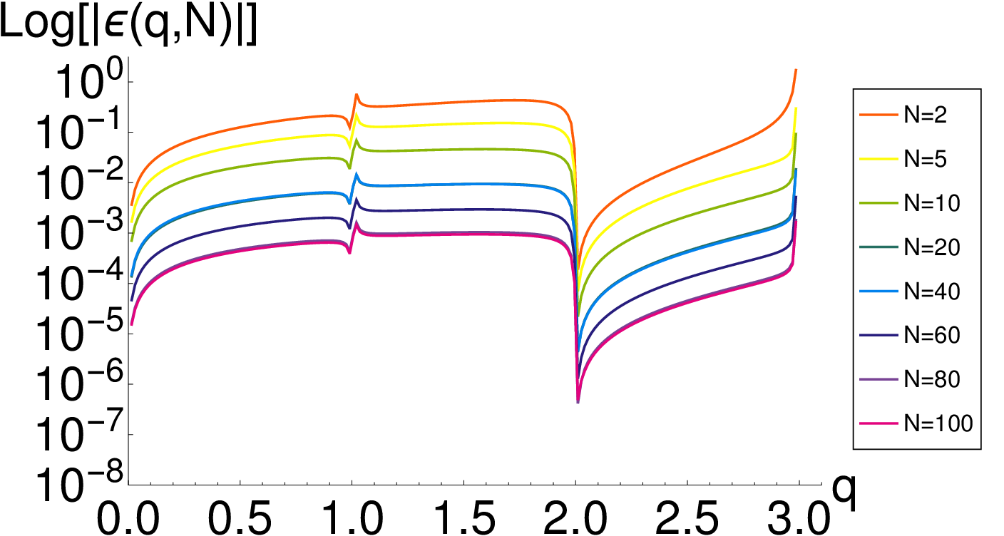
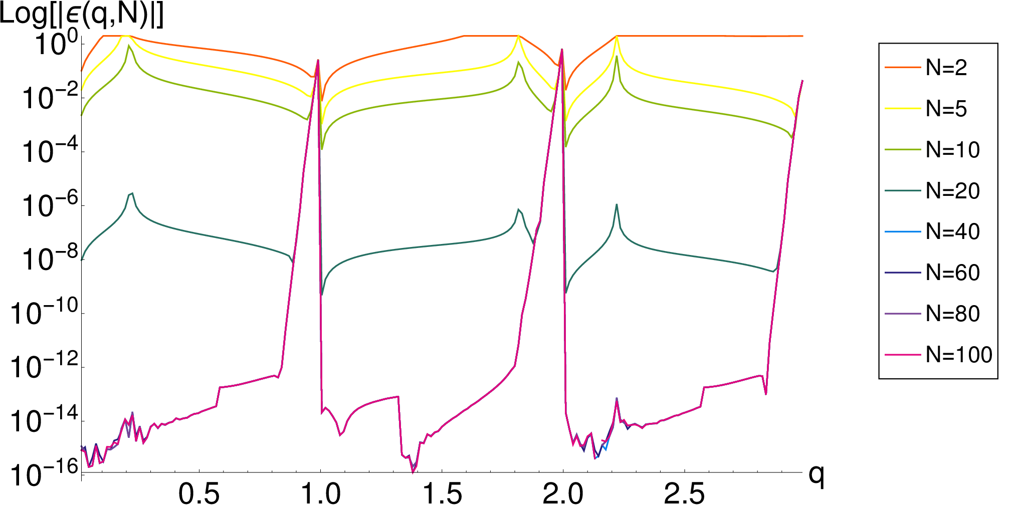
where is the infinite series given by Eq.(27) and is the truncated series, where is the order of the fractional differential operator, and is the number of terms in the truncated series Eq.(27). We observe spikes in the log-error, , either in case of real-valued roots of the fractional derivative or its approximation , or in the case of a match between the fractional derivative and its approximation. Yet another discontinuity in the error arises if the fractional derivative and its approximation are of equal magnitude but opposite in sign.
To approximate the fractional derivative of hyperbolic secant to within , we need to keep only the first three terms, as can be seen in Fig.(2). We note that a traditional approach in the evaluation of a fractional derivative of hyperbolic secant (tangent) relies on the Taylor series expansion, which diverges at due to a pole in the complex plane [16]. The divergence of the Taylor series results in the divergence of Riemann–Liouville and Caputo fractional derivatives if it is directly used in the integration process. However, the infinite series representation of the fractional derivative of and given by Eq.(19) is formulated in terms of integer derivatives of the original function, and does not depend on the properties of the Taylor series. Thus, the integer derivative series for the Grünwald–-Letnikov fractional derivative of hyperbolic secant and hyperbolic tangent functions has an infinite radius of convergence, as can be seen in Fig.(1). The log-linear plot of truncation error in the fractional derivative of and is shown in Fig.(2).
For functions described by Taylor series with an infinite radius of convergence, e.g., and , the number of terms needed to reach a given level of accuracy depends on the distance away from the base point used in the integer derivative expansion. For example, to approximate the Caputo fractional derivative on , we need to retain the first terms to reach accuracy in the same domain as for the fractional derivative on the hyperbolic secant, as can be seen in Fig.(3).
While for a certain class of functions the integer derivative series given by Eq.(19) improves the fractional derivative approximation with every additional term, the integer derivative expansion of a fractional derivative of a Gaussian function diverges for finite orders of , as we show below in Fig.(4). We note that the finite sum is convergent only in a vicinity around the origin and at infinity due to the Gaussian envelope. Indeed, our integer derivative expansion given by Eq.(19) for the Grünwald–-Letnikov fractional derivative of can be expressed in terms of Hermite polynomials , i.e.
| (29) | |||
This sum inherits large oscillations from the Hermite polynomials for both large values of its argument and its index . These oscillations result in a divergence of the integer derivative expansion, and thus, establish limits of the universality of the main result Eq.(19).






V Solving linear fractional differential equations with constant and variable coefficients using truncated series
In the previous section we established convergence of the Grünwald–-Letnikov fractional derivative by truncating the infinite integer derivative series and retaining only the first three terms. The goal of this section is to apply the truncated expansion of a fractional derivative to solve linear fractional differential equations (FDEs) with constant and variable coefficients. We choose two simplest non-trivial FDEs, which have solutions in terms of special functions, e.g. Mittag-Leffler and generalized Fox-Wright functions. The comparison of the numerical approximation to the exact analytic result provides a direct test for the robustness of the numerical scheme based on the truncated expansion of a fractional derivative.
The simplest form of the linear fractional differential equation with constant coefficients is given by
| (30) |
where is a real-valued constant. The exact solution of Eq.(30) is given in terms of the generalized Mittag-Leffler function [1] defined as
| (31) |
Specifically, the solution to Eq.(30) is given by [12]
| (32) |
By adopting the Caputo fractional derivative, which ensures a solution convergent at the origin, and retaining the first terms in the integer derivative expansion, Eq.(27), for a fractional order , we obtain a second order differential equation,
| (33) |
The solution of the transformed differential equation is subject to the boundary conditions,
| (34) | |||
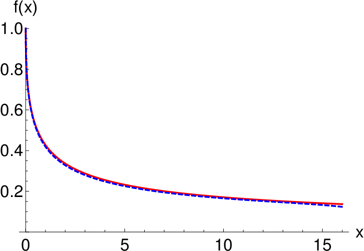
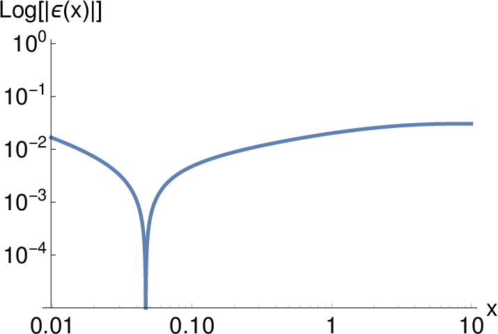
The numerical solution of Eq.(33) is readily obtained via a fourth-order Runge-Kutta iterative method, shown in Fig.(5) along with the relative truncation error defined in Eq.(28).
Next we turn to a linear fractional differential equation with variable coefficients,
| (35) |
The exact solution to the fractional differential equation Eq.(35) is given in terms of the generalized Fox-Wright function [1],
| (36) |
In particular, the solution to Eq.(35) is given by
| (37) |
where is an arbitrary real constant. In the special case of the fractional order the generalized Fox-Wright function is reduced to a Gaussian function,
| (38) |
| (39) |
where in the argument of the Fox-Wright function stands for an absent argument.


As a result the solution to the fractional differential equation Eq.(35) in the special case of is
| (40) |
If we further specify , we fix the constant and obtain the exact solution to Eq.(35),
| (41) |
By retaining the first terms in the integer derivative expansion Eq.(27), we acquire,
| (42) |
If we change variables according to , we obtain a transformed differential equation,
| (43) |
We specify the initial conditions as,
| (44) | ||||
and apply a fourth-order Runge-Kutta iterative method to find the numerical solution of Eq.(43). The result along with the relative truncation error is shown in Fig.(6).
In this section, we successfully demonstrated that expanding a fractional derivative in terms of integer order derivatives is a robust method for solving linear fractional differential equations with both constant and variable coefficients. In the special case of a differential equation with variable coefficients, the truncated series with only the first terms leads to a error, while the very same truncation applied to a differential equation with constant coefficients results in a error. Although this method cannot be exhaustively tested for all possible fractional orders of differential operators and all types of FDEs, linear FDEs, considered in this work, constitute a large sample that can be used in many physical applications where the response of a system is proportional to a fractional order parameter [10, 11, 12]. Thus, the numerical scheme based on the truncated integer derivative expansion is a powerful method for solving a broad range of linear FDEs.
VI Conclusions
In this paper we expressed the Grünwald–-Letnikov fractional derivative as an infinite sum of integer order derivatives. We compared the obtained infinite expansion with the corresponding series produced by the Riemann–Liouville and Caputo definitions of a fractional derivative. We found that all three definitions are represented by the very same infinite series, with the exception of the lower index of summation for the Caputo fractional derivative which accounts for the initial conditions at the expansion point. Thus, we have shown that the integer derivative series representation provides a unified description for various definitions of a fractional derivative.
By truncating the infinite expansion and retaining only the first few terms, we demonstrated the convergence of the Grünwald–-Letnikov fractional derivative. We have shown that for functions represented by Taylor series with an infinite radius of convergence, the truncation error decreases with an increasing number of terms kept in the truncated expansion. We emphasized that the infinite expansion does not rely on the properties of the Taylor series, which has profound consequences for the functions characterized by a finite radius of convergence of the corresponding Taylor series. Specifically, we have shown that the infinite series of integer order derivatives for hyperbolic secant and tangent functions has an infinite radius of convergence, compared to the corresponding Taylor series with a finite radius of convergence of . However, for a Gaussian function we found that the infinite expansion is divergent due to the factorial growth and oscillatory nature of the Hermite polynomials. Thus, the Gaussian function establishes limits of the universality of the infinite expansion of the Grünwald–-Letnikov fractional derivative in terms of integer order derivatives.
Finally, we applied the truncated series for a fractional derivative to solve linear fractional differential equations with both constant and variable coefficients. We found that the fourth-order Runge-Kutta method applied to truncated fractional differential equations results in numerical solutions that rapidly converge to the exact solutions given in terms of Mittag-Leffler and generalized Fox-Wright special functions. Thus, we concluded that the integer derivative expansion can be adapted to a robust numerical method for solving linear fractional differential equations, such as the fractional Schrödinger and fractional diffusion equations.
Acknowledgements.
The authors would like to thank David Benson, Daniel Jaschke, Nathan Smith, and Marc Valdez for numerous and fruitful discussions. A.G., G.S. and L.D.C. acknowledge support from the US National Science Foundation under grant numbers PHY-1306638, PHY-1207881, PHY-1520915, and OAC-1740130, and the US Air Force Office of Scientific Research grant number FA9550-14-1-0287. This work was performed in part at the Aspen Center for Physics, which is supported by National Science Foundation grant PHY-1607611. U.A. acknowledges support from UAEU-UPAR(4) and UAEU-UPAR(7).References
- [1] Anatoly A Kilbas, Hari M Srivastava, and Juan J Trujillo, Theory and Applications of Fractional Differential Equations (Elsevier, 2006).
- [2] Stefan G Samko, Anatoly A Kilbas, and Oleg I Marichev, Fractional integrals and derivatives: Theory and Applications (Gordon and Breach, 1993).
- [3] Jean-Philippe Bouchaud and Antoine Georges, “Anomalous diffusion in disordered media: statistical mechanisms, models and physical applications,” Phys. Rep. 195, 127–293 (1990).
- [4] Shlomo Havlin and Daniel Ben-Avraham, “Diffusion in disordered media,” Adv. Phys. 36, 695–798 (1987).
- [5] David A Benson, Mark M Meerschaert, and Jordan Revielle, “Fractional calculus in hydrologic modeling: A numerical perspective,” Adv. Wat. Res. 51, 479–497 (2013).
- [6] Rina Schumer, David A Benson, Mark M Meerschaert, and Boris Baeumer, “Multiscaling fractional advection-dispersion equations and their solutions,” Wat. Res. Research 39 (2003).
- [7] Rina Schumer, David A Benson, Mark M Meerschaert, and Stephen W Wheatcraft, “Eulerian derivation of the fractional advection–dispersion equation,” J. of Contaminant Hydrology 48, 69–88 (2001).
- [8] Diego del Castillo-Negrete, BA Carreras, and VE Lynch, “Front dynamics in reaction-diffusion systems with levy flights: a fractional diffusion approach,” Phys. Rev. Lett. 91, 018302 (2003).
- [9] John Kim and Parviz Moin, “Application of a fractional-step method to incompressible navier-stokes equations,” J. of Comp. Phys. 59, 308–323 (1985).
- [10] Rudolf Hilfer, Applications of fractional calculus in physics (World Scientific, 2000).
- [11] Bruce J West, “Colloquium: Fractional calculus view of complexity: A tutorial,” Rev. Mod. Phys. 86, 1169 (2014).
- [12] Richard Herrmann, Fractional calculus: an introduction for physicists (World Scientific, 2014).
- [13] Brian N Lundstrom, Matthew H Higgs, William J Spain, and Adrienne L Fairhall, “Fractional differentiation by neocortical pyramidal neurons,” Nat. Neuroscience 11, 1335–1342 (2008).
- [14] Thomas J Anastasio, “The fractional-order dynamics of brainstem vestibulo-oculomotor neurons,” Biol. Cybernetics 72, 69–79 (1994).
- [15] L. D. Landau and E. M. Lifshitz, “Quantum mechanics: non-relativistic theory,” (1958).
- [16] James Ward Brown and Ruel Churchill, Complex variables and applications. (Boston: McGraw-Hill Higher Education, 2009).