A family of compact semitoric systems with two focus-focus singularitiesThanks: The first author was partially supported by the Research Fund of the University of Antwerp and the second author is partially supported by an AMS-Simons travel grant.

Abstract.

About 6 years ago, semitoric systems were classified by Pelayo $\&$ Vũ Ngọc by means of five invariants. Standard examples are the coupled spin oscillator on ${\mathbb{S}}^{2}\times{\mathbb{R}}^{2}$ and coupled angular momenta on ${\mathbb{S}}^{2}\times{\mathbb{S}}^{2}$ , both having exactly one focus-focus singularity. But so far there were no explicit examples of systems with more than one focus-focus singularity which are semitoric in the sense of that classification. This paper introduces a $6$ -parameter family of integrable systems on ${\mathbb{S}}^{2}\times{\mathbb{S}}^{2}$ and proves that, for certain ranges of the parameters, it is a compact semitoric system with precisely two focus-focus singularities. Since the twisting index (one of the semitoric invariants) is related to the relationship between different focus-focus points, this paper provides systems for the future study of the twisting index.

Key words and phrases:

Symplectic geometry, integrable system, semitoric integrable system, Hamiltonian system, momentum map, focus-focus singularity.

1991 Mathematics Subject Classification

Primary: 37J35; Secondary: 53D20.

Sonja Hohloch

University of Antwerp

Department of Mathematics and Computer Science

Middelheimlaan 1

B-2020 Antwerpen, Belgium

Joseph Palmer

Rutgers University

Department of Mathematics

Hill Center - Busch Campus

110 Frelinghuysen Road

Piscataway, NJ 08854, USA.

1. Introduction

An integrable system is a triple $(M,\omega,F)$ where $(M,\omega)$ is a $2n$ -dimensional symplectic manifold and $F\colon M\to{\mathbb{R}}^{n}$ is a smooth function, known as the momentum map, whose components Poisson commute and are linearly independent almost everywhere. The points at which the linear independence fails are known as singular points. An integrable system is toric if $M$ is compact and the Hamiltonian vector fields of the components all have periodic flow of the same period; in this case the image of the momentum map $F(M)$ is a convex $n$ -dimensional polytope (a special case of the Atiyah-Guillemin-Sternberg Theorem [2, 12]) and additionally, by the work of Delzant [7], $F(M)$ completely determines the system $(M,\omega,F)$ up to equivariant symplectomorphism.

So-called semitoric integrable systems are a special class of integrable systems on $4$ -manifolds for which one of the two components of its momentum map has a Hamiltonian vector field with periodic flow. Specifically, a semitoric integrable system is an integrable system $(M,\omega,F=(J,H))$ such that $J$ is proper with periodic flow and every singular point is nondegenerate with no hyperbolic blocks (see Section 2 for a discussion of types of singular points). Semitoric integrable systems can have singular points of focus-focus type, which do not occur in toric integrable systems, and are an example of almost toric manifolds which were introduced by Symington [32].

Semitoric integrable systems were studied and classified by Pelayo $\&$ Vũ Ngọc [25, 26]. The classification is in terms of five invariants: the number of focus-focus points (which is finite according to Vũ Ngọc [35]); an infinite family of polygons known as a semitoric polygon; a Taylor series in two variables for each focus-focus point; the height of the focus-focus value in the semitoric polygon; and the twisting index, which, roughly, is an integer for each pair of focus-focus points describing the ‘twist’ of the singular Lagrangian fibration between them. Semitoric systems are rigid enough to admit a classification, but flexible enough to appear more frequently in physical examples and to admit more interesting dynamics. The main reason semitoric systems exhibit more interesting behavior than toric systems is the presence of the focus-focus points and the monodromy that these singularities can produce in the integral affine structure of the momentum map image $F(M)$ .

While the Pelayo-Vũ Ngọc classification predicts many systems and gives certain properties of those systems, one thing that has thus far been lacking are explicit examples of semitoric systems giving the symplectic manifold $(M,\omega)$ and the momentum map $F$ . Le Floch $\&$ Pelayo [18] explicitly describe the coupled angular momenta system (originally described in [31], see Example 2.12) and details of the coupled spin oscillator (see Example 2.13) are spread over several papers. These systems each have exactly one focus-focus singularity. In the present work we describe semitoric systems on $M={\mathbb{S}}^{2}\times{\mathbb{S}}^{2}$ which have two focus-focus singular points, generalizing the system from [18]. More precisely, the main result of this paper is the following.

Theorem 1.1.

Let $M={\mathbb{S}}^{2}\times{\mathbb{S}}^{2}$ be equipped with the symplectic form $\omega=-(R_{1}\omega_{{\mathbb{S}}^{2}}\oplus R_{2}\omega_{{\mathbb{S}}^{2}})$ where $\omega_{{\mathbb{S}}^{2}}$ is the standard volume form on the sphere and $0<R_{1}<R_{2}$ are real numbers. For $\vec{R}:=(R_{1},R_{2})$ and $\vec{t}:=(t_{1},t_{2},t_{3},t_{4})\in{\mathbb{R}}^{4}$ define $J_{\vec{R}},H_{\vec{t}}\ \colon M\to{\mathbb{R}}$ by

(1)

\begin{cases}J_{\vec{R}}(x_{1},y_{1},z_{1},x_{2},y_{2},z_{2}):=R_{1}z_{1}+R_{2}z_{2},\\ H_{\vec{t}}\ (x_{1},y_{1},z_{1},x_{2},y_{2},z_{2}):=t_{1}z_{1}+t_{2}z_{2}+t_{3}(x_{1}x_{2}+y_{1}y_{2})+t_{4}z_{1}z_{2}\end{cases}

where $(x_{i},y_{i},z_{i})$ are Cartesian coordinates on ${\mathbb{S}}^{2}\subset{\mathbb{R}}^{3}$ for $i=1,2$ . Then there exist choices of $t_{1},t_{2},t_{3},t_{4},R_{1},R_{2}$ such that $(M,\omega,(J_{\vec{R}},H_{\vec{t}}))$ is a semitoric system with exactly two focus-focus points.

Theorem 1.1 is restated in more detail in Section 3 as Theorem 3.1. The coupled angular momenta system with coupling parameter $t\in\ ]0,1[$ is the special case of Equation (1) with $t_{1}=t$ , $t_{3}=t_{4}=1-t$ , and $t_{2}=0$ . The coupled angular momenta system describes the rotation of two vectors (with magnitudes $R_{1}$ and $R_{2}$ ) about the $z$ -axis and has as a second integral a linear combination of the $z$ -component of the first vector and the inner produce of the two vectors, while the system in Equation (1) includes additionally the $z$ -component of the second vector and also breaks the inner product into two components, namely the projection to the $z$ -axis and the projection to the $xy$ -plane.

The system in Equation (1) is studied from a different point of view in mathematical physics, where it is a special case of a generalized Gaudin model. We refer the interested reader to Petrera’s PhD thesis [29] and the references therein for the development since Gaudin’s original work [11].

Theorem 1.1 gives explicit global formulas (defined by the same expression on the entire manifold) for a family of examples of semitoric systems with more than one focus-focus point. This family should be useful for understanding semitoric systems at a concrete, computationally amenable, context. The twisting index invariant is related to the relationship between different focus-focus singular points, so having an example with multiple focus-focus points will help in understanding this invariant (though it does actually appear in a more subtle way for systems with only one focus-focus point).

Additionally, not only the system itself, but also the method by which we produce this system is of interest. We construct it as a linear combination of four different systems of toric type (semitoric systems with no focus-focus points) and in this way one can see how it deforms into each of these four systems (see Figure 1) which correspond to four elements of the associated semitoric polygon. Let $N$ denote the north pole of ${\mathbb{S}}^{2}$ and $S$ denote the south pole, so that $(N,N)$ , $(N,S)$ , $(S,N)$ , and $(S,S)$ are the four possible products of poles in ${\mathbb{S}}^{2}\times{\mathbb{S}}^{2}$ . The next theorem follows from Theorem 4.4 in Section 4, in which we take $R_{1}=1$ and $R_{2}=2$ for simplicity.

Theorem 1.2.

For $s_{1},s_{2}\in[0,1]$ let $(J_{\vec{R}},H_{(s_{1},s_{2})})$ denote the system $(J_{\vec{R}},H_{\vec{t}})$ where

t_{1}=(1-s_{1})(1-s_{2}),\qquad t_{2}=s_{1}s_{2},\qquad t_{3}=s_{1}+s_{2}-2s_{1}s_{2},\qquad t_{4}=s_{1}-s_{2}.

Then $(J_{(1,2)},H_{(s_{1},s_{2})})$ has the following properties:

1)

it is an integrable system for all $(s_{1},s_{2})\in[0,1]^{2}$ ;
2)

it is a semitoric system when $(s_{1},s_{2})\in[0,1]^{2}\setminus\gamma$ where $\gamma\subset[0,1]^{2}$ is the union of four smooth curves;
3)

the points $(N,S),(S,N)\in\mathbb{S}^{2}\times\mathbb{S}^{2}$ transition between being elliptic-elliptic, focus-focus, and degenerate depending on the value of $(s_{1},s_{2})$ ;
4)

it is semitoric with exactly two focus-focus points for all $(s_{1},s_{2})$ in an open neighborhood of $\left(\frac{1}{2},\frac{1}{2}\right)$ ;
5)

it is semitoric with no focus-focus point if $(s_{1},s_{2})\in\{(0,0),(0,1),(1,0),(1,1)\}$ .

The set $\gamma$ represents the moment at which singular points become degenerate while they change between focus-focus and elliptic-elliptic type. Proposition 2.8 states that if the type of a singular point changes from focus-focus to elliptic-elliptic by smoothly varying the integrals (on a fixed manifold) then it must become degenerate during the transition, in fact, it is undergoing a Hamiltonian-Hopf bifurcation, see Remark 2.9. The set $\gamma$ is an intersection of zero sets of discriminants of certain polynomials, see Equation (23). The image of the momentum map for the system in Theorem 1.2 is plotted in Figure 1 for various choices of $(s_{1},s_{2})$ and $\gamma$ is plotted in Figure 2. The coupled angular momenta system from Le Floch $\&$ Pelayo [18] is exactly the one parameter family of systems obtained from the system in Theorem 1.2 by taking $s_{2}=0$ , so the momentum map image of the coupled angular momentum system is the bottom row of images in Figure 1.

Figure 1. An image of the momentum map

(J_{(1,2)},H_{(s_{1},s_{2})})

with the rank 0 points marked for varying values of

s_{1},s_{2}\in[0,1]

. Notice that the coupled angular momenta system shown in Figure 3 is the bottom row of the system shown in this figure since the coupled angular momenta is the special case for which

s_{2}=0

Figure 2. Left: a plot of the set

\gamma

, which is the union of

\gamma_{(S,N)}

(blue) and

\gamma_{(N,S)}

(orange), see Equation 23. Right: Values of

(s_{1},s_{2})

for which the system

(J_{(1,2)},H_{(s_{1},s_{2})})

has focus-focus values at: only the point

(S,N)

(blue), only the point

(N,S)

(orange), or at both points (green). The system is degenerate on the black curves. Compare with Figure 1.

Recently there has been a lot of activity relating to semitoric integrable systems, which we review briefly now. There has been work regarding quantizations of semitoric integrable systems, specifically related to the problem of recovering the classical system from the quantum one (see for instance Le Floch $\&$ Pelayo $\&$ Vũ Ngọc [19]). Hohloch $\&$ Sabatini $\&$ Sepe [13] answer the question of how the classification of semitoric systems is linked to Karshon’s classification [17] of Hamiltonian ${\mathbb{S}}^{1}$ -spaces. The question of lifting a Hamiltonian ${\mathbb{S}}^{1}$ -action to a semitoric system is an ongoing project by Hohloch $\&$ Sabatini $\&$ Sepe $\&$ Symington and has been the topic of several conference talks. There has been work to determine the convexity of the momentum map image with respect to its intrinsic integral affine structure by Ratiu $\&$ Wacheux $\&$ Zung [30]. Alonso $\&$ Dullin $\&$ Hohloch [1] are computing higher order terms of the Taylor series invariant of the focus-focus point in the coupled spin-oscillator (Example 2.13 of the present paper). Deformations of semitoric systems have been studied by endowing the moduli space with a topology, see Palmer [22]. Kane $\&$ Palmer $\&$ Pelayo [15, 16] used combinatorial methods to study blowups/downs and minimal models of semitoric systems. Generalizations of semitoric systems are achieved in Pelayo $\&$ Ratiu $\&$ Vũ Ngọc [24] and Hohloch $\&$ Sabatini $\&$ Sepe $\&$ Symington [14]. Additionally, work has begun to extend the theory of semitoric systems to higher dimensional manifolds in Wacheux [36]. Surgery techniques for semitoric systems are an ongoing project by Hohloch $\&$ Sabatini $\&$ Sepe $\&$ Symington. Presently, hyperbolic singularities are excluded from semitoric integrable systems, but Dullin $\&$ Pelayo [8] have produced a smooth family of systems with transition from being semitoric to having a family of hyperbolic singular points. A reader new to integrable systems can consult the surveys Pelayo $\&$ Vũ Ngọc [27] and Pelayo [23], or the books Marsden $\&$ Ratiu [20] and Cushman $\&$ Bates [5].

Structure of the article:

In Section 2 we review the required background, including integrable systems, singular points, and semitoric integrable systems. In Section 3 we introduce the new system and prove Theorem 1.1. In Section 4 we discuss the choice of parameters for which the system can be seen as a linear combination of four systems of toric type, and prove Theorem 1.2.

Figures:

All figures and associated numerical computations in this article were made with the computer program Mathematica.

2. Fundamental definitions

In Section 2.1 we introduce standard notions related to integrable systems and non-degenerate points. A reader familiar with these topics can skip directly to Section 2.2.

2.1. Integrable systems and non-degenerate singular points

2.1.1. Integrable systems

Given a symplectic manifold $(M,\omega)$ recall that associated to any function $f\in C^{\infty}(M)$ there is a vector field denoted by $X^{f}$ , called the Hamiltonian vector field associated to $f$ , and defined by

\omega(X^{f},\cdot)=-df(\cdot).

Moreover, recall the Poisson bracket $\{\cdot,\cdot\}\colon C^{\infty}(M)\times C^{\infty}(M)\to C^{\infty}(M)$ given by $\{f,g\}=\omega(X^{f},X^{g})$ . An integrable system is a symplectic $2n$ -manifold $(M,\omega)$ along with a collection of functions $f_{1},\ldots,f_{n}$ which Poisson commute (i.e. $\{f_{i},f_{j}\}=0$ for all $i,j$ ) and for which the associated Hamiltonian vector fields $X^{f_{1}},\ldots,X^{f_{n}}$ are linearly independent almost everywhere. The function $F=(f_{1},\ldots,f_{n})\colon M\to{\mathbb{R}}^{n}$ is known as the momentum map of this system.

In this article, we will focus on the case $n=2$ , so an integrable system will be a $4$ -dimensional symplectic manifold $(M,\omega)$ with a function $F\colon(M,\omega)\to{\mathbb{R}}^{2}$ whose components $F=(J,H)$ are such that $\{J,H\}=0$ and $X^{J}(p)$ and $X^{H}(p)$ are linearly independent for almost all $p\in M$ .

The points at which linear independence of the components of the momentum map fails are known as the singular points of the system and the rank of a singular point is the rank of the differential of the momentum map $dF$ at that point. There is a natural notion of non-degeneracy for such singular points which we review now. Rank 0 singular points are known as fixed points since they are fixed under the flow of the Hamiltonian vector fields of the components of the momentum map; we will start with the classification of those.

2.1.2. Rank 0 singular points, i.e., fixed points

Let $p\in M$ be a fixed point and let $\mathcal{Q}(T_{p}M)$ denote the vector space of quadratic forms on $T_{p}M$ . The symplectic form on $M$ gives $\mathcal{Q}(T_{p}M)$ the structure of a Lie algebra which is isomorphic to $\mathfrak{sp}(4,{\mathbb{R}})$ , see Bolsinov $\&$ Fomenko [3]. Recall that a Cartan subalgebra is a nilpotent and self-normalizing subalgebra.

Definition 2.1.

A fixed point $p\in M$ is non-degenerate if the Hessians $d^{2}J(p)$ and $d^{2}H(p)$ span a Cartan subalgebra of the Lie algebra of quadratic forms on $T_{p}M$ .

In practice, this condition can be checked by use of the following lemma.

Lemma 2.2 (Bolsinov $\&$ Fomenko [3]).

Let $p\in M$ be a fixed point. Denote by $\omega_{p}$ the matrix of the symplectic form with respect to a basis of $T_{p}M$ and let $d^{2}J$ and $d^{2}H$ denote the matrices of the Hessians of $J$ and $H$ with respect to the same basis. Then $p$ is non-degenerate if and only if $d^{2}J$ and $d^{2}H$ are linearly independent and there exists a linear combination of $\omega_{p}^{-1}d^{2}J$ and $\omega_{p}^{-1}d^{2}H$ which has four distinct eigenvalues.

Sketch of proof.

The result follows from the fact that an abelian subalgebra of $\mathfrak{sp}(4,{\mathbb{R}})$ is a Cartan subalgebra if and only if it is two dimensional and contains a regular element, in which case it is the centralizer for this regular element. The span of $\omega_{p}^{-1}d^{2}J$ and $\omega_{p}^{-1}d^{2}H$ is an abelian subspace of $\mathfrak{sp}(T_{p}M)\cong\mathfrak{sp}(4,{\mathbb{R}})\cong\mathcal{Q}(T_{p}M)$ because $J$ and $H$ Poisson commute (since they form an integrable system) and a regular element is any matrix with four distinct eigenvalues. We conclude that if $\omega_{p}^{-1}d^{2}J$ and $\omega_{p}^{-1}d^{2}H$ are linearly independent and their span includes an element with four eigenvalues then the span is a two-dimensional abelian subalgebra which contains a regular element, and is thus Cartan. ∎

2.1.3. Rank 1 singular points

To define rank 1 non-degenerate singular points we will again follow Bolsinov $\&$ Fomenko [3, Section 1.8.2]. Suppose that $p$ is a singular point of rank 1 in a 4-dimensional integrable system $(M,\omega,F=(J,H))$ . Then there exists some $\mu,\lambda\in\mathbb{R}$ such that $\mu dH+\lambda dJ=0$ at $p$ and the $\mathbb{R}^{2}$ -action defined by flowing along the vector fields of $J$ and $H$ has a one-dimensional orbit through $p$ . Let $L\subset T_{p}M$ be the tangent line of this orbit at $p$ and let $L^{\prime}$ be the symplectic orthogonal complement to $L$ . Notice that $L\subset L^{\prime}$ and since $J$ and $H$ Poisson commute they are invariant under the ${\mathbb{R}}^{2}$ -action and thus the operator $\mu d^{2}H+\lambda d^{2}J$ descends to the quotient $L^{\prime}/L$ .

Definition 2.3 (Bolsinov $\&$ Fomenko [3]).

The rank 1 critical point $p$ is non-degenerate if $\mu d^{2}H+\lambda d^{2}J$ is invertible on $L^{\prime}/L$ .

Now suppose that the flow of $X^{J}$ is periodic. Recall that the symplectic quotient of $M$ by $J$ at the level $c$ , which we denote $M\sslash{\mathbb{S}}^{1}$ , is the symplectic manifold $J^{-1}(c)/{{\mathbb{S}}^{1}}$ where the ${{\mathbb{S}}^{1}}$ -action on $J^{-1}(c)$ is the one which comes from the flow of the Hamiltonian vector field of $J$ .

Lemma 2.4.

If $p\in M$ is a rank 1 singular point such that $dJ\neq 0$ then $p$ is non-degenerate if and only if $d^{2}H$ is invertible at the image of $p$ in the symplectic quotient of $M$ by $J$ at the level $J(p)$ .

Proof.

Let $L$ and $L^{\prime}$ be as above and let $c=J(p)$ . Notice that $dJ\neq 0$ and $\mathrm{dim}(L)=1$ implies that $L$ is spanned by $X^{J}$ . Thus $v\in L^{\prime}$ if and only if $\omega_{p}(v,X^{J})=0$ . By the definition of the Hamiltonian vector field this is equivalent to $v(J)=0$ , so $v\in T_{p}(J^{-1}(c))$ . Thus $L^{\prime}=T_{p}(J^{-1}(c))$ . Furthermore, $L$ is the tangent space to the orbit of the ${{\mathbb{S}}^{1}}$ -action through $p$ so $L^{\prime}/L=T_{p}(J^{-1}(c)/{{\mathbb{S}}^{1}})$ and the result follows. ∎

Lemma 2.4 implies the following.

Corollary 2.5.

If $dJ\neq 0$ at all points of nonzero rank then all rank 1 points of $(M,\omega,F=(J,H))$ are non-degenerate if and only if $H$ descends to a Morse function on all possible symplectic quotients by $J$ .

See Bolsinov $\&$ Fomenko [3] for a description of non-degenerate points for dimensions greater than four and a description of rank 1 non-degenerate points in terms of Cartan subalgebras.

2.1.4. Classification of non-degenerate points

Williamson [37] classified Cartan subalgebras of $\mathfrak{sp}(n,{\mathbb{R}})$ , which in turn implies a classification of the possible subalgebras $\mathfrak{c}$ generated by the Hessians in $T_{p}M\cong\mathfrak{sp}(n,{\mathbb{R}})$ at a non-degenerate singular points. Eliasson [10] and Miranda $\&$ Zung [21] extended Williamson’s pointwise classification to a local classification, which classifies the possible forms of the momentum map in local symplectic coordinates around a fixed point $p$ , often known as the Eliasson-Miranda-Zung normal form.

Theorem 2.6 (Eliasson [10], Miranda $\&$ Zung [21]).

If $p\in M$ is a non-degenerate singular point of an $n$ -dimensional integrable system $(M,\omega,F)$ then there exist local symplectic coordinates $(x,y):=(x_{1},\ldots,x_{n},y_{1},\ldots,y_{n})$ around $p$ such that there exist $q_{1},\ldots,q_{n}\colon M\to{\mathbb{R}}$ where each $q_{i}$ is given by one of:

1)

elliptic: $q_{i}(x,y)=\frac{1}{2}(x_{i}^{2}+y_{i}^{2})$ ,
2)

hyperbolic: $q_{i}(x,y)=x_{i}y_{i}$ ,
3)

focus-focus: $\begin{cases}q_{i}(x,y)=x_{i}y_{i+1}-x_{i+1}y_{i},\\ q_{i+1}(x,y)=x_{i}y_{i}+x_{i+1}y_{i+1},\end{cases}$
4)

non-singular: $q_{i}(x,y)=y_{i}$ ,

such that $\{f_{i},q_{j}\}=0$ for all $i,j$ .

The classification of a non-degenerate singular point can be detected by computing the eigenvalues of any associated regular element.

Proposition 2.7 (Vũ Ngọc [34, Chapter 3]).

If $A$ is a regular element in the Cartan subalgebra generated by the Hessians of the components of the momentum map (i.e., $A$ has $2n$ distinct eigenvalues) at a fixed point then the eigenvalues of $A$ come in three distinct types of groups:

1)

a pair of imaginary roots $\pm\mathrm{i}\beta$ , called an elliptic block,
2)

a pair of real roots $\pm\alpha$ , called a hyperbolic block,
3)

a quadruple of complex roots $\pm\alpha\pm\mathrm{i}\beta$ , called a focus-focus block,

where $\alpha,\beta\in{\mathbb{R}}$ .

The types of the groups of eigenvalues of $A$ agree with the classification of the Cartan subalgebra in Theorem 2.6. Thus they do not depend on the choice of the regular element $A$ , they only depend on the Cartan subalgebra.

2.1.5. Degenerate points

Changing the integrable system on a fixed symplectic manifold cannot cause a rank 0 point to transition from being focus-focus type to being elliptic-elliptic type without passing through a degeneracy.

Proposition 2.8.

Fix a $4$ -dimensional symplectic manifold $(M,\omega)$ . Let $t_{0}\in{\mathbb{R}}$ and let $J_{t},H_{t}\colon M\to{\mathbb{R}}$ be smooth functions which depend smoothly on $t\in{\mathbb{R}}$ . Suppose $(J_{t},H_{t})$ is an integrable system for all $t\in{\mathbb{R}}$ in an open interval around $t_{0}$ and $p\in M$ is a rank 0 fixed point of $(J_{t},H_{t})$ for all $t\in{\mathbb{R}}$ , which is of type elliptic-elliptic for $t>t_{0}$ and type focus-focus for $t<t_{0}$ . Then $(J_{t_{0}},H_{t_{0}})$ has a degenerate fixed point at $p$ .

Proof.

Suppose that $p$ is a non-degenerate fixed point of $(J_{t_{0}},H_{t_{0}})$ . Then there exists some $\gamma,\delta\in{\mathbb{R}}$ such that $\omega^{-1}(\gamma d^{2}H_{t_{0}}+\delta d^{2}J_{t_{0}})$ has four distinct eigenvalues at $p$ . Fix such $\gamma$ and $\delta$ . Since $\gamma d^{2}H_{t}+\delta d^{2}J_{t}$ is symmetric we see that the characteristic polynomial of $\omega^{-1}(\gamma d^{2}H_{t_{0}}+\delta d^{2}J)$ is a constant multiple of a polynomial of the form

g_{t}(X)=X^{4}+b_{t}X^{2}+c_{t}

where $b_{t},c_{t}\in{\mathbb{R}}$ depend continuously on $t$ . The zeros of $g_{t}$ are given by $\pm\sqrt{\kappa_{\pm}}$ where

\kappa_{\pm}=\frac{-b_{t}\pm\sqrt{b_{t}^{2}-4c_{t}}}{2}

and since there are four distinct eigenvalues when $t=t_{0}$ we see that $b_{t_{0}}^{2}-4c_{t_{0}}\neq 0$ . Thus we see that $g_{t}$ has four distinct eigenvalues for all $t$ in a neighborhood of $t_{0}$ . Since the Williamson type of a fixed point does not depend on the choice of linear combination as long as one with four distinct eigenvalues is chosen we see that $g_{t}$ has zeros of the form $\pm\mathrm{i}\alpha$ , $\pm\mathrm{i}\beta$ for $t>t_{0}$ which means that $b_{t}^{2}-4c_{t}>0$ . Similarly, we see that $g_{t}$ has zeros of the form $\alpha\pm\mathrm{i}\beta$ for $t<t_{0}$ which means that $b_{t}^{2}-4c_{t}<0$ . Thus, since $b_{t}-4c_{t}$ varies continuously with $t$ , we see that $b_{t_{0}}-4c_{t_{0}}=0$ contradicting our original claim. ∎

Similar arguments to the one in the proof of Proposition 2.8 are used in Dullin-Pelayo [8] and in particular in Figure 4 in that paper.

Remark 2.9.

When a point changes between being of elliptic-elliptic and focus-focus type it is undergoing what is known as the Hamiltonian-Hopf bifurcation, see [4].

We are grateful to Heinz Hanßmann and James Montaldi for bringing to our attention the Hamiltonian-Hopf bifurcation and informing us that our system is undergoing this transformation.

2.2. Semitoric systems

Pelayo $\&$ Vũ Ngọc [25, 26] extend the Delzant classification of toric integrable systems by introducing and classifying what are now known as semitoric systems.

Definition 2.10.

A semitoric system is a integrable system of dimension four $(M,\omega,(J,H))$ such that:

1)

$J$ is proper,
2)

the Hamiltonian flow of $J$ (i.e. the flow of $X^{J}$ ) is periodic,
3)

all singular points of $(J,H)$ are non-degenerate and have no hyperbolic blocks.

A semitoric system is simple if there is at most one critical point in $J^{-1}(x)$ for all $x\in{\mathbb{R}}$ .

Every semitoric system we consider in

this article is a simple semitoric system.

Note that $J$ is automatically proper in the case that $M$ is compact. Concerning item (2)), we may assume that $2\pi$ is the minimal period. Note that this means the flow of $X^{J}$ generates a faithful action of ${\mathbb{S}}^{1}={\mathbb{R}}/2\pi{\mathbb{Z}}$ .

If $(M,\omega,(J,H))$ is a semitoric integrable system and $p\in M$ is a rank zero singular point then there are exactly two possibilities for $p$ : either $p$ is elliptic-elliptic or focus-focus. Thus, if $A$ is a regular element in the associated Cartan subalgebra then the eigenvalues of $A$ must either come in two pairs $\pm\mathrm{i}\alpha$ , $\pm\mathrm{i}\beta$ in which case $p$ is elliptic-elliptic or come in one quadruple $\pm\alpha\pm\mathrm{i}\beta$ in which case $p$ is focus-focus, where $\alpha,\beta\in{\mathbb{R}}$ in each case. If $p$ is non-degenerate of rank 1 then it must be of elliptic type.

The Pelayo-Vũ Ngọc classification of simple semitoric integrable systems is in terms of five invariants, which we briefly describe now:

1)

the number of focus-focus points invariant: $m_{f}\in{\mathbb{Z}}_{\geq 0}$ denotes the number of focus-focus singular points (which is finite by Vũ Ngọc [35]),
2)

the semitoric polygon: a family of polygons (analogous to the Delzant polygon of a toric integrable system) which encode information about the integral-affine structure of the system. Each element is the image of a toric momentum map defined on all of $M$ except certain subsets (which are the union of submanifolds of dimension at most three) related to the focus-focus points,
3)

the Taylor series invariant: a Taylor series in two variables for each focus-focus point, which encodes the dynamics of the flow of the Hamiltonian vector fields as they approach the focus-focus fiber (originally introduced and described in Vũ Ngọc [33]),
4)

the volume or height invariant: a real number for each focus-focus point which encodes the height of the focus-focus value in semitoric polygon,
5)

the twisting index: an integer assigned to each focus-focus point for each element of the semitoric polygon, which encodes the relationship between the toric momentum map used to produce the element of the semitoric polygon and a preferred local momentum map around the focus-focus point.

An abstract list of such datas is known as a list of semitoric ingredients. Given semitoric systems $(M_{i},\omega_{i},(J_{i},H_{i}))$ for $i=1,2$ an isomorphism of semitoric systems is a symplectomorphism $\Phi\colon M_{1}\to M_{2}$ such that $\Phi^{*}(J_{2},H_{2})=(J_{1},f(J_{1},H_{1}))$ where $f\colon{\mathbb{R}}^{2}\to{\mathbb{R}}$ is a smooth function and $\partial_{y}f>0$ everywhere.

Theorem 2.11 (Classification by Pelayo $\&$ Vũ Ngọc [25, 26]).

The following hold:

1)

Two simple semitoric systems are isomorphic if and only if they have the same five semitoric invariants,
2)

Given a list of semitoric ingredients there exists a simple semitoric system which has those as its five invariants.

For standard examples of semitoric systems, we refer to Section 2.4.

2.3. The symplectic structure on ${\mathbb{S}}^{2}$ and ${\mathbb{S}}^{2}\times{\mathbb{S}}^{2}$

In order to avoid, on the one hand, confusion concerning the various conventions in the literature and, on the other hand, to provide a precise and complete reference, the following calculations are provided in full.

Let ${\mathbb{S}}^{2}$ be the unit sphere in ${\mathbb{R}}^{3}$ centered at the origin, and let $(x_{1},y_{1},z_{1},x_{2},y_{2},z_{2})$ be Cartesian coordinates on ${\mathbb{R}}^{3}\times{\mathbb{R}}^{3}$ . We consider the 4-dimensional manifold ${\mathbb{S}}^{2}\times{\mathbb{S}}^{2}\subset{\mathbb{R}}^{3}\times{\mathbb{R}}^{3}$ with symplectic form

\omega:=\omega^{R_{1}R_{2}}:=-(R_{1}\omega_{{\mathbb{S}}^{2}}\oplus R_{2}\omega_{{\mathbb{S}}^{2}})

where $R_{1},R_{2}\in{\mathbb{R}}^{>0}$ and $\omega_{{\mathbb{S}}^{2}}$ is the standard symplectic form on ${\mathbb{S}}^{2}$ . Geometrically, the symplectic form $\omega_{{\mathbb{S}}^{2}}$ on ${\mathbb{S}}^{2}$ is given in $p\in{\mathbb{S}}^{2}$ by

\displaystyle(\omega_{{\mathbb{S}}^{2}})_{p}(u,v)=\langle p,u\times v\rangle

where $\langle\cdot,\cdot\rangle$ is the Euclidean scalar product in ${\mathbb{R}}^{3}$ , $p=(p_{1},p_{2},p_{3})\in{\mathbb{S}}^{2}$ the basepoint and $u=(u_{1},u_{2},u_{3}),v=(v_{1},v_{2},v_{3})\in T_{p}{\mathbb{S}}^{2}$ tangent vectors, i.e., $\langle p,u\rangle=0=\langle p,v\rangle$ . To express $\omega_{{\mathbb{S}}^{2}}$ in Cartesian coordinates, we calculate

	$\displaystyle\langle p,u\times v\rangle$	$\displaystyle=p_{1}\det\begin{pmatrix}u_{2}&v_{2}\\ u_{3}&v_{3}\end{pmatrix}+p_{2}\det\begin{pmatrix}u_{3}&v_{3}\\ u_{1}&v_{1}\end{pmatrix}+p_{3}\det\begin{pmatrix}u_{1}&v_{1}\\ u_{2}&v_{2}\end{pmatrix}$
		$\displaystyle=p_{1}(dy\wedge dz)(u,v)+p_{2}(dz\wedge dx)(u,v)+p_{3}(dx\wedge dy)(u,v)$

and thus

\omega_{{\mathbb{S}}^{2}}=xdy\wedge dz+ydz\wedge dx+zdx\wedge dy.

This implies

\omega=-\sum_{i=1}^{2}R_{i}x_{i}dy_{i}\wedge dz_{i}+R_{i}y_{i}dz_{i}\wedge dx_{i}+R_{i}z_{i}dx_{i}\wedge dy_{i}

in Cartesian coordinates on ${\mathbb{S}}^{2}\times{\mathbb{S}}^{2}\subset{\mathbb{R}}^{3}\times{\mathbb{R}}^{3}$ . We want to use charts on ${\mathbb{S}}^{2}$ that parametrise the upper and lower hemisphere as graphs over the 2-dimensional unit disk ${\mathbb{D}}^{2}$ . To keep track of signs, we use $e\in\{+1,-1\}$ in the charts and have $\varphi_{e}:{\mathbb{D}}^{2}\to{\mathbb{S}}^{2}$ with

\varphi_{e}(x,y):=\left(x,y,z_{e}(x,y)\right):=\left(x,y,e\sqrt{1-x^{2}-y^{2}}\right)

such that $\varphi_{+1}$ covers the northern hemisphere and $\varphi_{-1}$ the southern one. Denoting the north and south pole of ${\mathbb{S}}^{2}$ by $N$ and $S$ , we get charts for the ‘double hemispheres’ around $(N,N),(N,S),(S,N),(S,S)\in{\mathbb{S}}^{2}\times{\mathbb{S}}^{2}$ via choosing $e_{1},e_{2}\in\{+1,-1\}$ accordingly and setting

(2)		$\displaystyle\varphi_{e_{1},e_{2}}$	$\displaystyle:{\mathbb{D}}^{2}\times{\mathbb{D}}^{2}\to{\mathbb{S}}^{2}\times{\mathbb{S}}^{2},$
	$\displaystyle\varphi_{e_{1}e_{2}}(x_{1},y_{1},x_{2},y_{2})$	$\displaystyle:=\left(x_{1},y_{1},e_{1}\sqrt{1-x_{1}^{2}-y_{1}^{2}},x_{2},y_{2},e_{2}\sqrt{1-x_{2}^{2}-y_{2}^{2}}\ \right).$

For better readability, let us drop the subscripts $e$ , $e_{1}$ , and $e_{2}$ whenever the context allows, and introduce a function $z_{i}(x_{i},y_{i})$ , i.e., we write

\varphi=\varphi_{e},\quad z(x,y)=e\sqrt{1-x^{2}-y^{2}},\quad\varphi=\varphi_{e_{1}e_{2}},\quad z_{i}(x_{i},y_{i}):=e_{i}\sqrt{1-x_{i}^{2}-y_{i}^{2}}

whenever possible. Now we express $\omega_{{\mathbb{S}}^{2}}$ in the new coordinates $\varphi_{e}$ . We compute

(3)		$\displaystyle\partial_{x}z(x,y)$	$\displaystyle=\frac{-ex}{\sqrt{1-x^{2}-y^{2}}}=\frac{-x}{z(x,y)}$
(4)		$\displaystyle\partial_{y}z(x,y)$	$\displaystyle=\frac{-ey}{\sqrt{1-x^{2}-y^{2}}}=\frac{-y}{z(x,y)}$

yielding

(5)

\displaystyle d(z(x,y))

\displaystyle=\frac{-x}{z(x,y)}dx+\frac{-y}{z(x,y)}dy

leading to

\displaystyle\varphi^{*}\omega_{{\mathbb{S}}^{2}}

\displaystyle=\left(\frac{x^{2}}{z(x,y)}+\frac{y^{2}}{z(x,y)}+z(x,y)\right)dx\wedge dy=\frac{1}{z(x,y)}dx\wedge dy.

Subsequently we get for $\omega$ in coordinates $\varphi=\varphi_{e_{1}e_{2}}$ the expression

	$\displaystyle\varphi^{*}\omega$	$\displaystyle=-\ \varphi^{*}(R_{1}\omega_{{\mathbb{S}}^{2}}\oplus R_{2}\omega_{{\mathbb{S}}^{2}})$
		$\displaystyle=-\left(\frac{R_{1}}{z_{1}(x_{1},y_{1})}\ dx_{1}\wedge dy_{1}+\frac{R_{2}}{z_{2}(x_{2},y_{2})}\ dx_{2}\wedge dy_{2}\right)$

and thus in matrix form we have

(6)

\displaystyle\omega=\begin{pmatrix}0&\frac{-R_{1}}{z_{1}}&0&0\\ \frac{R_{1}}{z_{1}}&0&0&0\\ 0&0&0&\frac{-R_{2}}{z_{2}}\\ 0&0&\frac{R_{2}}{z_{2}}&0\end{pmatrix}\qquad\textrm{and}\qquad\omega^{-1}=\begin{pmatrix}0&\frac{z_{1}}{R_{1}}&0&0\\ \frac{-z_{1}}{R_{1}}&0&0&0\\ 0&0&0&\frac{z_{2}}{R_{2}}\\ 0&0&\frac{-z_{2}}{R_{2}}&0\end{pmatrix}.

Suppose $f:{\mathbb{S}}^{2}\times{\mathbb{S}}^{2}\to{\mathbb{R}}$ . Using the charts $\varphi_{e_{1}e_{2}}$ , we compute for $h:=f\circ\varphi_{e_{1}e_{2}}:{\mathbb{D}}\times{\mathbb{D}}\to{\mathbb{R}}$ the differential

dh=\sum_{i=1}^{2}\partial_{x_{i}}h\ dx_{i}+\partial_{y_{i}}h\ dy_{i}

and can solve $\omega(X^{h},\cdot)=-dh$ for $X^{h}$ via

(X^{h})^{T}=-\begin{pmatrix}\partial_{x_{1}}h,\ \partial_{y_{1}}h,\partial_{x_{2}}h,\ \partial_{y_{2}}h\end{pmatrix}\ \omega^{-1}

(7)

X^{h}(x_{1},y_{1},x_{2},y_{2})=\begin{pmatrix}\frac{\partial_{y_{1}}h(x_{1},y_{1},x_{2},y_{2})\ z_{1}(x_{1},x_{2})}{R_{1}}\\ -\frac{\partial_{x_{1}}h(x_{1},y_{1},x_{2},y_{2})\ z_{1}(x_{1},x_{2})}{R_{1}}\\ \frac{\partial_{y_{2}}h(x_{1},y_{1},x_{2},y_{2})\ z_{2}(x_{2},y_{2})}{R_{2}}\\ -\frac{\partial_{x_{2}}h(x_{1},y_{1},x_{2},y_{2})\ z_{2}(x_{2},y_{2})}{R_{2}}\end{pmatrix}.

2.4. Explicit examples of semitoric systems

Consider the manifold ${\mathbb{S}}^{2}\times{\mathbb{S}}^{2}$ with symplectic form $\omega:=-(R_{1}\omega_{{\mathbb{S}}^{2}}\oplus R_{2}\omega_{{\mathbb{S}}^{2}})$ where $\omega_{{\mathbb{S}}^{2}}$ is the standard volume form on ${\mathbb{S}}^{2}$ and $0<R_{1}<R_{2}$ are real numbers.

Example 2.12 (Coupled angular momenta).

The coupled angular momenta system is given by $J_{\vec{R}},H_{t}\colon{\mathbb{S}}^{2}\times{\mathbb{S}}^{2}\to{\mathbb{R}}$ with

(8)

\begin{cases}J_{\vec{R}}(x_{1},y_{1},z_{1},x_{2},y_{2},z_{2}):=R_{1}z_{1}+R_{2}z_{2},\\ H_{t}(x_{1},y_{1},z_{1},x_{2},y_{2},z_{2}):=(1-t)z_{1}+t(x_{1}x_{2}+y_{1}y_{2}+z_{1}z_{2})\end{cases}

where $(x_{i},y_{i},z_{i})$ are Cartesian coordinates on ${\mathbb{S}}^{2}\subset{\mathbb{R}}^{3}$ for $i=1,2$ , $t\in[0,1]$ is the coupling parameter, and $\vec{R}=(R_{1},R_{2})\in{\mathbb{R}}^{2}$ with $0<R_{1}<R_{2}$ .

This system was originally introduced in Sadovskií $\&$ Zĥilinskií [31] and studied in detail in Le Floch $\&$ Pelayo [18], where it is shown that there exist two fixed values $t_{-},t_{+}\in(0,1)$ with $t_{-}<t_{+}$ which depend on $R_{1},R_{2}$ such that

1)

if $t_{-}<t<t_{+}$ then $(J_{\vec{R}},H_{t})$ is a semitoric system with exactly one focus-focus point,
2)

if $t>t_{+}$ or $t<t_{-}$ the $(J_{\vec{R}},H_{t})$ is a semitoric system with exactly zero focus-focus points (these are known as systems of toric type, see Section 2 of Vũ Ngọc [35]),
3)

if $t=t_{-}$ or $t=t_{+}$ then $(J_{\vec{R}},H_{t})$ has a degenerate singular point, and thus is not a semitoric system.

The image of the momentum map for Example 2.12 with varying values of $t$ is shown in Figure 3.

Figure 3. The momentum map image for the coupled angular momenta system with the rank zero points marked. As the coupling parameter

t

changes one of the rank zero points transitions from being elliptic-elliptic to being focus-focus and then back to elliptic-elliptic.

Another standard example of a semitoric system is

Example 2.13 (Coupled spin oscillator).

The coupled spin oscillator system is given by $J,H:{\mathbb{S}}^{2}\times{\mathbb{R}}^{2}\to{\mathbb{R}}$ where

\displaystyle J(x,y,z,u,v):=\frac{1}{2}(u^{2}+v^{2})+z\quad\mbox{and}\quad H(x,y,z,u,v)

\displaystyle:=\frac{1}{2}(ux+vy)

with Cartesian coordinates $(x,y,z)$ on ${\mathbb{S}}^{2}$ and $(u,v)$ on ${\mathbb{R}}^{2}$ .

See Pelayo $\&$ Vũ Ngọc [28] for a detailed investigation of Example 2.13.

Remark 2.14.

The spherical pendulum consists of $J,H:\mathrm{T}^{*}{\mathbb{S}}^{2}\to{\mathbb{R}}$ with

	$\displaystyle J(q_{1},q_{2},q_{3},p_{1},p_{2},p_{3})$	$\displaystyle:=q_{1}p_{2}-q_{2}p_{1},$
	$\displaystyle H(q_{1},q_{2},q_{3},p_{1},p_{2},p_{3})$	$\displaystyle:=\frac{1}{2}(p_{1}^{2}+p_{2}^{2}+p_{3}^{2})+q_{3}$

and satisfies nearly all of the requirements to be semitoric, but the $J$ is not proper since the momentum map image contains unbounded vertical lines. However, the spherical pendulum is a so-called generalized semitoric system, as discussed in Pelayo $\&$ Ratiu $\&$ Vũ Ngọc [24]. For this same reason, the quadratic spherical pendulum (see for example Cushman $\&$ Vũ Ngọc [6] and Efstathiou $\&$ Martynchuk [9]) is not a semitoric integrable system.

3. A family of systems with two focus-focus points

In this section we introduce the system which is the subject of this paper and prove Theorem 1.1, our main result. This system is minimal in the sense of Kane $\&$ Palmer $\&$ Pelayo [16], i.e., it is not possible to perform a blowdown of toric type on the system (see Kane $\&$ Palmer $\&$ Pelayo [16, Section 4.1] for a description of this operation). Minimal semitoric integrable systems are classified in Kane $\&$ Palmer $\&$ Pelayo [16] and the system discussed in the present paper is minimal of type (2), using the terminology of that paper.

3.1. The system

Consider $R_{1},R_{2}\in{\mathbb{R}}^{>0}$ as scaling of radii with $R_{1}<R_{2}$ and endow ${\mathbb{S}}^{2}\times{\mathbb{S}}^{2}$ with the symplectic form $\omega=\omega^{R_{1}R_{2}}$ . Let $\vec{t}:=(t_{1},t_{2},t_{3},t_{4})\in{\mathbb{R}}^{4}$ be parameters, let $\vec{R}=(R_{1},R_{2})$ , and define $\Phi:=(J_{\vec{R}},H_{\vec{t}}):{\mathbb{S}}^{2}\times{\mathbb{S}}^{2}\to{\mathbb{R}}^{2}$ in Cartesian coordinates by

\left\{\begin{aligned} J_{\vec{R}}(x_{1},y_{1},z_{1},x_{2},y_{2},z_{2})&:=R_{1}z_{1}+R_{2}z_{2},\\ H_{\vec{t}}(x_{1},y_{1},z_{1},x_{2},y_{2},z_{2})&:=t_{1}z_{1}+t_{2}z_{2}+t_{3}(x_{1}x_{2}+y_{1}y_{2})+t_{4}z_{1}z_{2}\end{aligned}\right.

as in Equation (1).

Unless we explicitly need the parameters we often write $J:=J_{\vec{R}}$ and $H:=H_{\vec{t}}$ for brevity. The main result of this section is

Theorem 3.1.

The following hold:

1)

The system (1) is a compact integrable system for all choices of parameters with $t_{3}\neq 0$ ,
2)

The system (1) is semitoric and has two focus-focus points for parameters in a neighborhood of

$R_{1}=1,\,\,R_{2}=2,\,\,t_{1}=\frac{1}{4},\,\,t_{2}=\frac{1}{4},\,\,t_{3}=\frac{1}{2},\,\,t_{4}=0.$

Theorem 3.1 is a combination of Propositions 3.9 and 3.13 and Corollary 3.15 which we prove in the remainder of this section.

Remark 3.2.

At the parameters for which the system in Equation (1) is has two focus-focus points it enjoys a certain sense of uniqueness. As shown in [16, Theorem 2.5], up to scaling the lengths of the sides, there is only one semitoric polygon for which the corresponding system is compact with two focus-focus points such that $J$ has isolated fixed points. Thus, this semitoric polygon is the one associated to the system in Equation (1). By evaluating $J$ on the rank zero points (see Lemma 3.4) we can easily find the semitoric polygon for the system (1), as shown in Figure 4.

Figure 4. Four semitoric polygons associated to the system (1). The slanted edges all have slope

\pm 1

. For each polygon the

x

-coordinates of the vertices, from left to right, are

-R_{1}-R_{2}

R_{1}-R_{2}

-R_{1}+R_{2}

, and

R_{1}+R_{2}

(since we assume

R_{1}<R_{2}

Remark 3.3.

At first, we considered the system

	$\displaystyle J_{\vec{R}}(x_{1},y_{1},z_{1},x_{2},y_{2},z_{2})$	$\displaystyle:=R_{1}z_{1}+R_{2}z_{2},$
	$\displaystyle H_{(\ell_{1},\ell_{2})}(x_{1},y_{1},z_{1},x_{2},y_{2},z_{2})$	$\displaystyle:=(1-\ell_{1})z_{1}+(1-\ell_{2})z_{2}+\ell_{1}\ell_{2}(x_{1}x_{2}+y_{1}y_{2}+z_{1}z_{2})$

for $\ell_{1},\ell_{2}\in[0,1]$ hoping to generalize the construction of the coupled angular momentum, but numerical evidence strongly suggests that while there are two different points that become focus-focus for certain values there is no choice of $\ell_{1}$ and $\ell_{2}$ for which both points are focus-focus simultaneously.

3.2. Rank 0 points and their nondegeneracy

In the chart $\varphi$ , the integrals $J$ and $H$ are given by

(9)		$\displaystyle J(x_{1},y_{1},x_{2},y_{2})$	$\displaystyle=R_{1}z_{1}+R_{2}z_{2},$
(10)		$\displaystyle H(x_{1},y_{1},x_{2},y_{2})$	$\displaystyle=t_{1}z_{1}+t_{2}z_{2}+t_{3}(x_{1}x_{2}+y_{1}y_{2})+t_{4}z_{1}z_{2}.$

where each $z_{i}=z_{i}(x_{i},y_{i})$ is a function of $x_{i}$ and $y_{i}$ for $i=1,2$ . Using equations (3), (4), and (7), the Hamiltonian vector fields are given by

(11)

X^{J}(x_{1},y_{1},x_{2},y_{2})=\begin{pmatrix}-y_{1}\\ x_{1}\\ -y_{2}\\ x_{2}\end{pmatrix},X^{H}(x_{1},y_{1},x_{2},y_{2})=\begin{pmatrix}\,\frac{-t_{1}y_{1}+t_{3}y_{2}z_{1}-t_{4}z_{2}y_{1}}{R_{1}}\\[6.0pt] \frac{t_{1}x_{1}-t_{3}x_{2}z_{1}+t_{4}z_{2}x_{1}}{R_{1}}\\[6.0pt] \frac{-t_{2}y_{2}+t_{3}y_{1}z_{2}-t_{4}z_{1}y_{2}}{R_{2}}\\[6.0pt] \frac{t_{2}x_{2}-t_{3}x_{1}z_{2}+t_{4}z_{1}x_{2}}{R_{2}}\end{pmatrix}.

Recall that $N$ denotes the north pole of ${\mathbb{S}}^{2}$ and $S$ the south pole.

Lemma 3.4.

The set of rank 0 points of $(J,H)$ , i.e., the set of fixed points, is given by $\{(N,N),(N,S),(S,N),(S,S)\}$ .

Proof.

Geometrically, $J$ is the sum of the height function on each factor of the product ${\mathbb{S}}^{2}\times{\mathbb{S}}^{2}$ scaled by $R_{1}$ and $R_{2}$ respectively. Thus $J$ gives rise to horizontal rotations on each of the two spheres and its Hamiltonian flow has fixed points exactly at $\{(N,N),(N,S),(S,N),(S,S)\}$ . The function $J$ reaches its global maximum, $R_{1}+R_{2}$ , at $(N,N)$ and its global minimum, $-(R_{1}+R_{2})$ , at $(S,S)$ . The corresponding fibers $J^{-1}(R_{1}+R_{2})$ and $J^{-1}(-(R_{1}+R_{2}))$ consist exactly of the singletons $\{(N,N)\}$ and $\{(S,S)\}$ .

Fixed points of $(J,H):{\mathbb{S}}^{2}\times{\mathbb{S}}^{2}\to{\mathbb{R}}$ require $\rk D(J,H)=0$ . Therefore they must have $DJ=0$ which is equivalent to $X^{J}=0$ , i.e., when we look for fixed points of $(J,H)$ , the only candidates are the points $(N,N)$ , $(N,S)$ , $(S,N)$ , and $(S,S)$ for which we have to check if additionally $DH=0$ or equivalently $X^{H}=0$ holds.

Since all possible fixed points lie in the range of the charts $\varphi_{e_{1}e_{2}}$ we can check the values of $X^{H}$ by using formula (3), (4), and (11). The corresponding point in the domain is in all cases $(x_{1},y_{1},x_{2},y_{2})=(0,0,0,0)$ and we compute that $X^{H}(0,0,0,0)$ vanishes and thus $\{(N,N),(N,S),(S,N),(S,S)\}$ is indeed the fixed point set of $(J,H)$ . ∎

Keep in mind from the above proof that the rank 0 points correspond to the origin in the charts in (2).

Lemma 3.5.

At the origin $p=(0,0,0,0)$ in the charts in (2), we find

(12)

\omega^{-1}_{p}d^{2}J(p)=\begin{pmatrix}0&-1&0&0\\ 1&0&0&0\\ 0&0&0&-1\\ 0&0&1&0\end{pmatrix}

and

(13)

\omega^{-1}_{p}d^{2}H(p)=\begin{pmatrix}0&-\frac{t_{1}+e_{2}t_{4}}{R_{1}}&0&\frac{e_{1}t_{3}}{R_{1}}\\ \frac{t_{1}+e_{2}t_{4}}{R_{1}}&0&-\frac{e_{1}t_{3}}{R_{1}}&0\\ 0&\frac{e_{2}t_{3}}{R_{2}}&0&-\frac{t_{2}+e_{1}t_{4}}{R_{2}}\\ -\frac{e_{2}t_{3}}{R_{2}}&0&\frac{t_{2}+e_{1}t_{4}}{R_{2}}&0\end{pmatrix}.

Proof.

We compute the Hessians of $J$ and $H$ using (9) and (10). Since derivatives are additive we can first calculate the Hessians of their components seperately. Recall from (3) and (4) that $\partial_{x_{i}}z_{i}=\frac{-x_{i}}{z_{i}}$ and $\partial_{y_{i}}z_{i}=\frac{-y_{i}}{z_{i}}$ , yielding

\displaystyle\partial^{2}_{x_{i}x_{i}}z_{i}=\frac{-z_{i}+x_{i}\partial_{x_{i}}z_{i}}{z_{i}^{2}},\quad\partial^{2}_{x_{i}y_{i}}z_{i}=\frac{x_{i}\partial_{y_{i}}z_{i}}{z_{i}^{2}},\quad\textrm{and}\quad\partial^{2}_{y_{i}y_{i}}z_{i}=\frac{-z_{i}+y_{i}\partial_{y_{i}}z_{i}}{z_{i}^{2}}.

Since $z_{1}$ does not depend on $x_{2},y_{2}$ and $z_{2}$ does not depend on $x_{1}$ and $y_{1}$ we obtain for the Hessian of $z_{i}$ w.r.t. the variables $x_{1}$ , $y_{1}$ , $x_{2}$ , $y_{2}$ in $p$

\displaystyle d^{2}z_{1}(p)=\begin{pmatrix}-e_{1}&0&0&0\\ 0&-e_{1}&0&0\\ 0&0&0&0\\ 0&0&0&0\end{pmatrix}\quad\mbox{and}\quad d^{2}z_{2}(p)=\begin{pmatrix}0&0&0&0\\ 0&0&0&0\\ 0&0&-e_{2}&0\\ 0&0&0&-e_{2}\\ \end{pmatrix}.

Next we consider the term $x_{1}x_{2}+y_{1}y_{2}$ and get

\displaystyle d^{2}(x_{1}x_{2}+y_{1}y_{2})(p)=\begin{pmatrix}0&0&1&0\\ 0&0&0&1\\ 1&0&0&0\\ 0&1&0&0\end{pmatrix}.

For the term $z_{1}z_{2}$ , we get

\displaystyle d^{2}(z_{1}z_{2})(p)=\begin{pmatrix}-e_{1}e_{2}&0&0&0\\ 0&-e_{1}e_{2}&0&0\\ 0&0&-e_{1}e_{2}&0\\ 0&0&0&-e_{1}e_{2}\end{pmatrix}.

The equations (9) and (10) together with the above calculations yield

\displaystyle d^{2}J(p)

\displaystyle=\begin{pmatrix}-e_{1}R_{1}&0&0&0\\ 0&-e_{1}R_{1}&0&0\\ 0&0&-e_{2}R_{2}&0\\ 0&0&0&-e_{2}R_{2}\end{pmatrix}

and

\displaystyle d^{2}H(p)

\displaystyle=\begin{pmatrix}-t_{1}e_{1}-t_{4}e_{1}e_{2}&0&t_{3}&0\\ 0&-t_{1}e_{1}-t_{4}e_{1}e_{2}&0&t_{3}\\ t_{3}&0&-t_{2}e_{2}-t_{4}e_{1}e_{2}&0\\ 0&t_{3}&0&-t_{2}e_{2}-t_{4}e_{1}e_{2}\end{pmatrix}.

Evaluating $\omega^{-1}$ from (6) at $p$ yields

\omega^{-1}_{p}=\begin{pmatrix}0&\frac{e_{1}}{R_{1}}&0&0\\ -\frac{e_{1}}{R_{1}}&0&0&0\\ 0&0&0&\frac{e_{2}}{R_{2}}\\ 0&0&-\frac{e_{2}}{R_{2}}&0\end{pmatrix}

and therefore, using $e_{1}^{2}=1=e_{2}^{2}$ , we get the desired results for $\omega_{p}^{-1}J(p)$ and $\omega_{p}^{-1}H(p)$ . ∎

Given a polynomial of the form $ay^{2}+by+c$ , the expression $b^{2}-4ac$ is called the discriminant of the polynomial. Thus, a straightforward calculation yields

Corollary 3.6.

Denote by $I$ the $4\times 4$ identity matrix. Then the characteristic polynomial of $\omega^{-1}_{p}d^{2}H(p)$ is given by

	$\displaystyle\chi(X)$	$\displaystyle:=\det\bigl(\omega^{-1}_{p}d^{2}H(p)-XI\bigr)$
		$\displaystyle=X^{4}+\frac{1}{R_{1}^{2}R_{2}^{2}}\left(R_{1}^{2}(t_{2}+e_{1}t_{4})^{2}+2e_{1}e_{2}R_{1}R_{2}t_{3}^{2}+R_{2}^{2}(t_{1}+e_{2}t_{4})^{2}\right)X^{2}$
		$\displaystyle\quad+\frac{1}{R_{1}^{2}R_{2}^{2}}\left((t_{2}+e_{1}t_{4})^{2}(t_{1}+e_{2}t_{4})^{2}-2e_{1}e_{2}(t_{2}+e_{1}t_{4})(t_{1}+e_{2}t_{4})t_{3}^{2}+t_{3}^{4}\right)$

which is a polynomial of second degree in $Y:=X^{2}$ with discriminant

(14)		$\displaystyle\triangle:=$	$\displaystyle\triangle_{\vec{R},\vec{t},e_{1},e_{2}}$
	$\displaystyle=$	$\displaystyle\left(\frac{1}{R_{1}^{2}R_{2}^{2}}\left(R_{1}^{2}(t_{2}+e_{1}t_{4})^{2}+2e_{1}e_{2}R_{1}R_{2}t_{3}^{2}+R_{2}^{2}(t_{1}+e_{2}t_{4})^{2}\right)\right)^{2}$
		$\displaystyle\quad-\frac{4}{R_{1}^{2}R_{2}^{2}}\left((t_{2}+e_{1}t_{4})^{2}(t_{1}+e_{2}t_{4})^{2}-2e_{1}e_{2}(t_{2}+e_{1}t_{4})(t_{1}+e_{2}t_{4})t_{3}^{2}+t_{3}^{4}\right).$

Now we want to determine the type of the rank $0$ points located at $(N,N)$ , $(N,S)$ , $(S,N)$ , $(S,S)$ , i.e., if they are nondegenerate or not and, in case they are nondegenerate, if they are focus-focus or elliptic-elliptic or something else. We will see that the type of the rank $0$ points highly depends on the choice of parameters $\vec{R}$ and $\vec{t}$ .

Proposition 3.7 (Rank 0 Criterion).

Suppose $p\in\mathbb{S}^{2}\times\mathbb{S}^{2}$ has $z$ -coordinates $(e_{1},e_{2})\in\{-1,1\}^{2}$ . Then $p$ is a rank 0 singular point of $(J_{\vec{R}},H_{\vec{t}})$ . If $\triangle_{\vec{R},\vec{t},e_{1},e_{2}}<0$ then $p$ is non-degenerate of focus-focus type, and if $\triangle_{\vec{R},\vec{t},e_{1},e_{2}}>0$ then $p$ is non-degenerate and is of type elliptic-elliptic, elliptic-hyperbolic, or hyperbolic-hyperbolic.

Proof.

We already know that the set of rank 0 point are exactly those with $z$ -coordinates $\pm 1$ by Lemma 3.4. Note that the characteristic polynomial of $\omega^{-1}_{p}d^{2}H(p)$ has zeros

X=\pm\sqrt{\frac{-1}{2R_{1}^{2}R_{2}^{2}}\left(R_{1}^{2}(t_{2}+e_{1}t_{4})^{2}+2e_{1}e_{2}R_{1}R_{2}t_{3}^{2}+R_{2}^{2}(t_{1}+e_{2}t_{4})^{2}\right)\pm\frac{\sqrt{\triangle}}{2}}

where $\triangle:=\triangle_{\vec{R},\vec{t},e_{1},e_{2}}$ is as in Equation (14).

If $\triangle<0$ then there are four eigenvalues which take the form $\alpha\pm\mathrm{i}\beta$ for $\alpha,\beta\in{\mathbb{R}}$ , and thus $p$ is focus-focus by Proposition 2.7. If, $\triangle>0$ then $p$ is a non-degenerate fixed point which is not focus-focus, so it is either elliptic-elliptic, hyperbolic-hyperbolic, or hyperbolic-elliptic. ∎

Note that in the case $\triangle=0$ the point can still be non-degenerate, but Proposition 3.7 does not give us any information in this case. The following statement implies that there exist parameter values for which the system has four nondegenerate rank $0$ points, two of them elliptic-elliptic and two focus-focus, and is proved by plugging the values into the criterion in Proposition 3.7.

Corollary 3.8.

For the parameter values

(15)

R_{1}=1,\quad R_{2}=2,\quad t_{1}=\frac{1}{4},\quad t_{2}=\frac{1}{4},\quad t_{3}=\frac{1}{2},\quad t_{4}=0,

the matrix $\omega^{-1}_{p}d^{2}H(p)$ has four distinct eigenvalues at each of the points $p\in\{(N,N),(S,S),(N,S),(S,N)\}$ given by

	$\displaystyle Eig(N,N)=Eig(S,S)=$	$\displaystyle\left\{\pm\frac{\mathrm{i}}{8}\sqrt{\frac{21+3\sqrt{33}}{2}},\,\pm\frac{\mathrm{i}}{8}\sqrt{\frac{21-3\sqrt{33}}{2}}\right\},$
	$\displaystyle Eig(N,S)=Eig(S,N)=$	$\displaystyle\left\{\left(\sqrt{\frac{5}{32}}\right)\left(\pm\cos\left(\frac{1}{2}\mathrm{arctan}\left(\frac{3\sqrt{31}}{11}\right)\right)\right.\right.$
		$\displaystyle\left.\left.\pm\mathrm{i}\sin\left(\frac{1}{2}\mathrm{arctan}\left(\frac{3\sqrt{31}}{11}\right)\right)\right)\right\},$

and thus $p$ is a nondegenerate fixed point according to Lemma 2.2. In particular, $(N,N)$ and $(S,S)$ are elliptic-elliptic and $(N,S)$ and $(S,N)$ are focus-focus.

Since nonvanishing and noncoinciding are open conditions, there exist in fact intervals around the parameters (15) where the systems continues to have two focus-focus and two elliptic-elliptic points.

Proposition 3.9.

There exists an open set $U\subset{\mathbb{R}}^{6}$ which contains the point $(1,2,\frac{1}{4},\frac{1}{4},\frac{1}{2},0)$ such that for all $(R_{1},R_{2},t_{1},t_{2},t_{3},t_{4})\in U$ the system given in Equation (1) has elliptic-elliptic points at $(N,N)$ and $(S,S)$ and focus-focus points at $(N,S)$ and $(S,N)$ .

3.3. Rank 1 points

We want to study rank 1 points by means of cylindrical coordinates. To avoid the problems with cylindrical coordinates near poles we state the following observation.

Lemma 3.10.

Let $t_{1}$ , $t_{2}$ , $t_{3}$ , $t_{4}\in{\mathbb{R}}$ , with $t_{3}\neq 0$ and let $R_{1}$ , $R_{2}\in{\mathbb{R}}^{>0}$ . If $(x_{1},y_{1},z_{1},x_{1},y_{2},z_{2})\in{\mathbb{S}}^{2}\times{\mathbb{S}}^{2}$ is a critical point of rank 1 of (1) then $z_{1},z_{2}\neq\{\pm 1\}$ .

Proof.

Critical points of $(J,H)$ from (1) are those $p\in{\mathbb{S}}^{2}\times{\mathbb{S}}^{2}$ such that $dH(p)$ and $dJ(p)$ are linearly dependent, which is equivalent to the existence of a nonzero $\lambda\in{\mathbb{R}}$ such that $d(H-\lambda J)(p)=0$ since $dJ=0$ only occurs at the rank 0 points. Defining $f_{1},f_{2}:{\mathbb{R}}^{6}\to{\mathbb{R}}$ by $f_{i}(x_{1},y_{1},z_{1},x_{2},y_{2},z_{2}):=x_{i}^{2}+y_{i}^{2}+z_{i}^{2}$ for $i=1,2$ , this is equivalent to looking for critical points of $H-\lambda J:{\mathbb{R}}^{6}\to{\mathbb{R}}$ on the set $f_{1}^{-1}(1)\cap f^{-1}_{2}(1)$ , i.e., critical points can be computed by means of Lagrangian multipliers, i.e., a critical point $p:=(x_{1},y_{1},z_{1},x_{1},y_{2},z_{2})$ satisfies the equations

\displaystyle\left\{\begin{aligned} &\nabla H(p)=\lambda\nabla J(p)+\mu_{1}\nabla f_{1}(p)+\mu_{2}\nabla f_{2}(p),\\ &x_{1}^{2}+y_{1}^{2}+z_{1}^{2}=1,\\ &x_{2}^{2}+y_{2}^{2}+z_{2}^{2}=1\end{aligned}\right.

for some $\lambda,\mu_{1},\mu_{2}\in{\mathbb{R}}$ . Using the gradient with respect to the Euclidean metric, we obtain

(16)

\displaystyle\begin{pmatrix}t_{3}x_{2}\\ t_{3}y_{2}\\ t_{1}+t_{4}z_{2}\\ t_{3}x_{1}\\ t_{3}y_{1}\\ t_{2}+t_{4}z_{1}\end{pmatrix}=\begin{pmatrix}0\\ 0\\ \lambda R_{1}\\ 0\\ 0\\ \lambda R_{2}\end{pmatrix}+\begin{pmatrix}2\mu_{1}x_{1}\\ 2\mu_{1}y_{1}\\ 2\mu_{1}z_{1}\\ 0\\ 0\\ 0\end{pmatrix}+\begin{pmatrix}0\\ 0\\ 0\\ 2\mu_{2}x_{2}\\ 2\mu_{2}y_{2}\\ 2\mu_{2}z_{2}\end{pmatrix}.

Recall that the rank 0 points are precisely those with $z_{1}\in\{\pm 1\}$ and $z_{2}\in\{\pm 1\}$ simultaneously. Suppose that $z_{1}\in\{\pm 1\}$ which implies $x_{1}=y_{1}=0$ since $(x_{1},y_{2},z_{1})\in{\mathbb{S}}^{2}$ . Then, recalling that $t_{3}\neq 0$ , we see that Equation (16) implies $x_{2}=y_{2}=0$ which in turn implies $z_{2}\in\{\pm 1\}$ so the only solution is in fact a rank 0 point. The same argument works if we assume $z_{2}\in\{\pm 1\}$ . ∎

We now introduce cylindrical coordinates on ${\mathbb{S}}^{2}\times{\mathbb{S}}^{2}$ via

(x_{i},y_{i},z_{i})\mapsto\begin{pmatrix}\sqrt{1-z_{i}^{2}}\cos(\theta_{i}),&\sqrt{1-z_{i}^{2}}\sin(\theta_{i}),&z_{i}\end{pmatrix}

where $i\in\{1,2\}$ and $\theta_{i}$ is the counterclockwise angle between the $x_{i}$ -axis and $(x_{i},y_{i})$ in ${\mathbb{R}}^{2}$ . In these coordinates, the system (1) becomes

	$\displaystyle J(\theta_{1},z_{1},\theta_{2},z_{2})$	$\displaystyle=R_{1}z_{1}+R_{2}z_{2},$
	$\displaystyle H(\theta_{1},z_{1},\theta_{2},z_{2})$	$\displaystyle=t_{1}z_{1}+t_{2}z_{2}+t_{3}\sqrt{(1-z_{1}^{2})(1-z_{2}^{2})}\cos(\theta_{1}-\theta_{2})+t_{4}z_{1}z_{2}$

and the symplectic form is

(17)

\omega=R_{1}dz_{1}\wedge d\theta_{1}+R_{2}dz_{2}\wedge d\theta_{2}.

According to Lemma 3.10 these coordinates are valid where rank 1 points may occur (if the rank 1 point occurs at the discontinuity of $\theta_{i}$ , then shift the domain of definition of $\theta_{i}$ ). We compute the derivative

(18)

\displaystyle dJ(\theta_{1},z_{1},\theta_{2},z_{2})=\begin{pmatrix}0,&R_{1},&0,&R_{2}\end{pmatrix}

which never vanishes. Therefore we have Corollary 2.5 at our disposal.

Let us compute the symplectic quotient $({\mathbb{S}}^{2}\times{\mathbb{S}}^{2})\sslash{\mathbb{S}}^{1}$ where the ${\mathbb{S}}^{1}$ -action is induced by $J$ . Given $c\in\ ]-(R_{1}+R_{2}),(R_{1}+R_{2})[$ , which is the set of regular values of $J$ , we can solve for $z_{1}$ on the level set $J^{-1}(c)$ to find

z_{1}=\frac{c-R_{2}z_{2}}{R_{1}}.

By Equations (18) and (17) we see that $X^{J}=\partial_{z_{1}}+\partial_{z_{2}}$ so the flow of $J$ rotates $\theta_{1}$ and $\theta_{2}$ by a common angle. Thus, the ${\mathbb{S}}^{1}$ -action produced by the flow of $X^{J}$ preserves the angle difference $\theta_{1}-\theta_{2}$ . Now consider the chart on the quotient $J^{-1}(c)/{\mathbb{S}}^{1}$ with coordinates $(\zeta,\vartheta)$ given by

\displaystyle\zeta:=z_{1}\quad\mbox{and}\quad\vartheta:=\theta_{1}-\theta_{2}

where

-1<\zeta<1\qquad\textrm{and}\qquad\frac{c-R_{2}}{R_{1}}<\zeta<\frac{c+R_{2}}{R_{1}}

since $-1<z_{1},z_{2}<1$ . All rank 1 critical points occur in this chart since by Lemma 3.10 rank 1 points do not occur when $z_{1}=\pm 1$ or $z_{2}=\pm 1$ . We now let $H$ descend to the symplectic quotient $({\mathbb{S}}^{2}\times{\mathbb{S}}^{2})\sslash{\mathbb{S}}^{1}$ where it reads

		$\displaystyle H(\zeta,\vartheta)$
		$\displaystyle=t_{1}\zeta+t_{2}\frac{c-R_{1}\zeta}{R_{2}}+t_{3}\cos(\vartheta)\sqrt{(1-\zeta^{2})\left(1-\left(\frac{c-R_{1}\zeta}{R_{2}}\right)^{2}\right)}+t_{4}\frac{c-R_{1}\zeta}{R_{2}}\zeta$
		$\displaystyle=\frac{t_{2}c}{R_{2}}+\frac{t_{1}R_{2}-t_{2}R_{1}+t_{4}c}{R_{2}}\zeta-\frac{t_{4}R_{1}}{R_{2}}\zeta^{2}+t_{3}\cos(\vartheta)\sqrt{(1-\zeta^{2})\left(1-\left(\frac{c-R_{1}\zeta}{R_{2}}\right)^{2}\right)}.$

We abbreviate the term under the last root by

A(\zeta):=A(\zeta,c,R_{1},R_{2}):=(1-\zeta^{2})\left(1-\left(\frac{c-R_{1}\zeta}{R_{2}}\right)^{2}\right)

and its derivatives with respect to $\zeta$ by

A^{\prime}:=\partial_{\zeta}A\qquad\textrm{and}\qquad A^{\prime\prime}:=\partial_{\zeta\zeta}^{2}A.

We note $A(\zeta)\geq 0$ with $A(\zeta)=0$ if and only if $\zeta=\pm 1$ or $\zeta=\frac{c\pm R_{2}}{R_{1}}$ . Because of the bounds on $\zeta$ we always have $A(\zeta)>0$ . In order to find the critical points of $H$ on the symplectic quotient we calculate the partial derivatives

	$\displaystyle\partial_{\vartheta}H(\zeta,\vartheta)$	$\displaystyle=-t_{3}\sin(\vartheta)\sqrt{A(\zeta)},$
	$\displaystyle\partial_{\zeta}H(\zeta,\vartheta)$	$\displaystyle=\frac{t_{1}R_{2}-t_{2}R_{1}+t_{4}c}{R_{2}}-\frac{2t_{4}R_{1}}{R_{2}}\zeta+t_{3}\cos(\vartheta)\frac{A^{\prime}(\zeta)}{2\sqrt{A(\zeta)}}.$

Lemma 3.11.

$(\zeta,\vartheta)$ is a critical point of $H$ on the symplectic quotient if and only if

\vartheta\in\pi{\mathbb{Z}}\quad\mbox{and}\quad 0=t_{1}R_{2}-t_{2}R_{1}+t_{4}c-2t_{4}R_{1}\zeta+t_{3}R_{2}\cos(\vartheta)\frac{A^{\prime}(\zeta)}{2\sqrt{A(\zeta)}}.

Proof.

The point $(\zeta,\vartheta)$ is critical if and only if $\partial_{\vartheta}H(\zeta,\vartheta)=0=\partial_{\zeta}H(\zeta,\vartheta)$ . Since $A(\zeta)$ and $t_{3}$ are nonzero $\partial_{\zeta}H(\zeta,\vartheta)=0$ is equivalent to $\sin(\vartheta)=0$ meaning $\vartheta\in\pi{\mathbb{Z}}$ and $\cos(\vartheta)=\pm 1$ . Together with $\partial_{\vartheta}H(\zeta,\vartheta)=0$ we get the desired result. ∎

3.4. Integrability

We consider the system (1) in the chart $\varphi=\varphi_{e_{1}e_{2}}$ defined in (2). By means of (7), we obtain as Hamiltonian vector fields in these coordinates

\displaystyle X^{x_{i}}=-\frac{z_{i}}{R_{i}}\partial_{y_{i}},\quad X^{y_{i}}=\frac{z_{i}}{R_{i}}\partial_{x_{i}},\quad X^{z_{i}}=-\frac{y_{i}}{R_{i}}\partial_{x_{i}}+\frac{x_{i}}{R_{i}}\partial_{y_{i}}

for $i\in\{1,2\}$ . Moreover, we deduce from (5)

dz_{i}=\frac{-x_{i}}{z_{i}}dx_{i}+\frac{-y_{i}}{z_{i}}dy_{i}.

This yields

(19)

\left\{\quad\begin{aligned} \{z_{i},x_{i}\}&=-dz_{i}(X^{x_{i}})=-\frac{y_{i}}{R_{i}},\\ \{z_{i},y_{i}\}&=-dz_{i}(X^{y_{i}})=\frac{x_{i}}{R_{i}},\\ \{z_{i},x_{j}\}&=\{z_{i},y_{j}\}=0\quad\mbox{for }i\neq j,\\ \{z_{i},z_{i}\}&=-dz_{i}(X^{z_{i}})=-\frac{x_{i}y_{i}}{R_{i}z_{i}}+\frac{x_{i}y_{i}}{R_{i}z_{i}}=0,\\ \{z_{1},z_{2}\}&=-dz_{1}(X^{z_{2}})=0.\end{aligned}\right.

Now we are ready to show

Lemma 3.12.

$\{J,H\}=0$ for all $R_{1},R_{2}\in{\mathbb{R}}^{>0}$ and all $t=(t_{1},t_{2},t_{3},t_{4})\in{\mathbb{R}}^{4}$ .

Proof.

We recall that the Poisson bracket is linear and that we have the identities in (19). Then we compute in the coordinates given in (2)

	$\displaystyle\{J,H\}$	$\displaystyle=\{R_{1}z_{1}+R_{2}z_{2},\ t_{1}z_{1}+t_{2}z_{2}+t_{3}(x_{1}x_{2}+y_{1}y_{2})+t_{4}z_{1}z_{2}\}$
		$\displaystyle\stackrel{{\scriptstyle\eqref{poissonCalc}}}{{=}}R_{1}(t_{3}\{z_{1},x_{1}x_{2}\}+t_{3}\{z_{1},y_{1}y_{2}\}+t_{4}\{z_{1},z_{1}z_{2}\})$
		$\displaystyle\quad+R_{2}(t_{3}\{z_{2},x_{1}x_{2}\}+t_{3}\{z_{2},y_{1}y_{2}\}+t_{4}\{z_{2},z_{1}z_{2}\}).$

Since the Poisson bracket satisfies the product rule $\{a,bc\}=\{a,b\}c+\{a,c\}b$ it follows

\displaystyle\stackrel{{\scriptstyle\eqref{poissonCalc}}}{{=}}R_{1}\left(t_{3}\left(\frac{-y_{1}}{R_{1}}x_{2}+\frac{x_{1}}{R_{1}}y_{2}\right)\right)+R_{2}\left(t_{3}\left(\frac{-y_{2}}{R_{2}}x_{1}+\frac{x_{2}}{R_{2}}y_{1}\right)\right)=0.

The charts in (2) are not defined for $z_{i}=0$ . To show $\{J,H\}=0$ there, consider Cartesian coordinates $(x_{1},y_{1},z_{1},x_{2},y_{2},z_{2})$ and choose charts given by

(x_{1},z_{1},x_{2},z_{2})\mapsto\left(x_{1},e_{1}\sqrt{1-x_{1}^{2}-z_{1}^{2}},z_{1},x_{2},e_{2}\sqrt{1-x_{2}^{2}-z_{2}^{2}},z_{2}\ \right)

etc. The calculations are completely analogous. ∎

Proposition 3.13.

The system $({\mathbb{S}}^{2}\times{\mathbb{S}}^{2},\omega,(J_{\vec{R}},H_{\vec{t}}))$ given in Equation (1) is integrable for all parameter values with $0<R_{1}<R_{2}$ and $t_{1},t_{2},t_{3},t_{4}\in{\mathbb{R}}$ with $t_{3}\neq 0$ .

Proof.

Fix parameter values and let $J=J_{(R_{1},R_{2})}$ and $H=H_{(t_{1},t_{2},t_{3},t_{4})}$ with $t_{3}\neq 0$ . In Lemma 3.12 we showed that $\{J,H\}=0$ . It follows from Lemma 3.11 and the fact that $t_{3}\neq 0$ that the rank 1 critical points occupy a set of measure zero since there are only finitely many on each symplectic quotient. By Lemma 3.4 there are only finitely many rank 0 points and thus $J$ and $H$ are linearly independent almost everywhere. ∎

3.5. Nondegeneracy of rank 1 points

Now we want to study nondegeneracy of the rank $1$ critical points. Therefore we have to compute the Hessian of $H$ on the symplectic quotient. We get

	$\displaystyle\partial^{2}_{\vartheta\vartheta}H(\zeta,\vartheta)$	$\displaystyle=-t_{3}\cos(\vartheta)\sqrt{A(\zeta)},$
	$\displaystyle\partial^{2}_{\vartheta\zeta}H(\zeta,\vartheta)$	$\displaystyle=-t_{3}\sin(\vartheta)\frac{A^{\prime}(\zeta)}{2\sqrt{A(\zeta)}},$
	$\displaystyle\partial^{2}_{\zeta\zeta}H(\zeta,\vartheta)$	$\displaystyle=-\frac{2t_{4}R_{1}}{R_{2}}+\frac{t_{3}\cos(\vartheta)}{2}\ \frac{A^{\prime\prime}(\zeta)\sqrt{A(\zeta)}-A^{\prime}(\zeta)\frac{A^{\prime}(\zeta)}{2\sqrt{A(\zeta)}}}{A(\zeta)}$
		$\displaystyle=\frac{-2t_{4}R_{1}}{R_{2}}+t_{3}\cos(\vartheta)\ \frac{2A^{\prime\prime}(\zeta)A(\zeta)-(A^{\prime}(\zeta))^{2}}{4(A(\zeta))^{\frac{3}{2}}}$

Now we come to a criterion for nondegeneracy. Let $pr_{c}\colon J^{-1}(c)\to J^{-1}(c)/\mathbb{S}^{1}$ denote the quotient map for each $c\in J(\mathbb{S}^{2}\times\mathbb{S}^{2})$ .

Proposition 3.14 (Rank 1 Criterion).

Suppose $p\in\mathbb{S}^{2}\times\mathbb{S}^{2}$ is a rank 1 critical point and denote $c=J(p)$ and $pr_{c}(p)=(\zeta,\vartheta)$ . Then $p$ is non-degenerate if and only if $\partial^{2}_{\zeta\zeta}H(\zeta,\vartheta)\neq 0$ . In particular, $p$ is non-degenerate and of elliptic-regular type if

\frac{2t_{4}R_{1}}{t_{3}R_{2}}\cos(\vartheta)>\frac{2A^{\prime\prime}(\zeta)A(\zeta)-(A^{\prime}(\zeta))^{2}}{4(A(\zeta))^{\frac{3}{2}}},

non-degenerate and of hyperbolic-regular type if

\frac{2t_{4}R_{1}}{t_{3}R_{2}}\cos(\vartheta)<\frac{2A^{\prime\prime}(\zeta)A(\zeta)-(A^{\prime}(\zeta))^{2}}{4(A(\zeta))^{\frac{3}{2}}},

and degenerate otherwise.

Proof.

We start by computing the symplectic form on the symplectic quotient. Let $j\colon J^{-1}(c)\to\mathbb{S}^{2}\times\mathbb{S}^{2}$ be the inclusion map. Recall $\omega=\sum_{i=1}^{2}R_{i}dz_{i}\wedge d\theta_{i}$ so we have

j^{*}\omega=R_{1}dz_{1}\wedge d\theta_{1}+R_{2}d\left(\frac{c-R_{1}z_{1}}{R_{2}}\right)\wedge d\theta_{2}=R_{1}dz_{1}\wedge d(\theta_{1}-\theta_{2})

and thus on the reduced space $\mathbb{S}^{2}\times\mathbb{S}^{2}\sslash\mathbb{S}^{1}$ in the coordinates $(\zeta,\vartheta)$ we have the symplectic form

\omega_{\mathrm{red}}=R_{1}d\zeta\wedge d\vartheta\qquad\textrm{with matrix}\qquad\omega_{\mathrm{red}}=R_{1}\begin{pmatrix}0&1\\ -1&0\end{pmatrix}.

Since $(\zeta,\vartheta)$ is a critical point Lemma 3.11 implies that $\sin(\vartheta)=0$ , so $\partial_{\vartheta\zeta}H(\zeta,\vartheta)=0$ and thus

	$\displaystyle\omega_{\mathrm{red}}^{-1}d^{2}H(\zeta,\vartheta)$	$\displaystyle=\frac{1}{R_{1}}\begin{pmatrix}0&-1\\ 1&0\end{pmatrix}\begin{pmatrix}\partial^{2}_{\zeta\zeta}H(\zeta,\vartheta)&0\\ 0&\partial^{2}_{\vartheta\vartheta}H(\zeta,\vartheta)\end{pmatrix}$
		$\displaystyle=\frac{1}{R_{1}}\begin{pmatrix}0&-\partial_{\theta\theta}^{2}H(\zeta,\vartheta)\\ \partial_{\zeta\zeta}^{2}H(\zeta,\vartheta)&0\end{pmatrix}$

which has eigenvalues

\lambda_{\pm}=\pm\frac{1}{R_{1}}\sqrt{-\partial^{2}_{\zeta\zeta}H(\zeta,\vartheta)\partial^{2}_{\vartheta\vartheta}H(\zeta,\vartheta)}.

Since $\cos(\vartheta)=\pm 1$ we see that $\partial^{2}_{\vartheta\vartheta}H(\zeta,\vartheta)\neq 0$ and so the eigenvalues are distinct if and only if $\partial^{2}_{\zeta\zeta}H(\zeta,\vartheta)\neq 0$ , establishing the first part of the claim. To complete the proof we notice that $\lambda_{\pm}$ are purely imaginary if $\partial^{2}_{\zeta\zeta}H(\zeta,\vartheta)\partial^{2}_{\vartheta\vartheta}H(\zeta,\vartheta)>0$ , which implies that $p$ is elliptic-regular, and purely real otherwise, implying that $p$ is hyperbolic-regular. We compute

		$\displaystyle\partial^{2}_{\zeta\zeta}H(\zeta,\vartheta)\partial^{2}_{\vartheta\vartheta}H(\zeta,\vartheta)$
		$\displaystyle=\left(\frac{-2t_{4}R_{1}}{R_{2}}+t_{3}\cos(\vartheta)\ \frac{2A^{\prime\prime}(\zeta)A(\zeta)-(A^{\prime}(\zeta))^{2}}{4(A(\zeta))^{\frac{3}{2}}}\right)\left(-t_{3}\cos(\vartheta)\sqrt{A(\zeta)}\right)$
		$\displaystyle=\sqrt{A(\zeta)}\left(\frac{2t_{3}t_{4}R_{1}}{R_{2}}\cos(\vartheta)-t_{3}^{2}\ \frac{2A^{\prime\prime}(\zeta)A(\zeta)-(A^{\prime}(\zeta))^{2}}{4(A(\zeta))^{\frac{3}{2}}}\right),$

and the result follows because $\sqrt{A(\zeta)}>0$ for the bounds on $\zeta$ . ∎

The following is established by plugging the specific values into the inequality from Proposition 3.14 (for more details see the proof of Lemma 4.2).

Corollary 3.15.

For the parameter values

(20)

R_{1}=1,\quad R_{2}=2,\quad t_{1}=\frac{1}{4},\quad t_{2}=\frac{1}{4},\quad t_{3}=\frac{1}{2},\quad t_{4}=0,

all rank 1 points are non-degenerate and of elliptic-regular type.

4. A linear combination of systems of toric type

In this section we apply the results of the previous section to a special choice of parameters of the system. Let $\vec{s}:=(s_{1},s_{2})\in[0,1]^{2}$ and consider the system $(J_{\vec{R}},H_{\vec{s}})$ on ${\mathbb{S}}^{2}\times{\mathbb{S}}^{2}$ using the same $J_{\vec{R}}$ as before but using $H_{\vec{s}}:=H_{\vec{t}}$ where

t_{1}=(1-s_{1})(1-s_{2}),\qquad t_{2}=s_{1}s_{2},\qquad t_{3}=s_{1}+s_{2}-2s_{1}s_{2},\qquad t_{4}=s_{1}-s_{2},

i.e., we consider

(21)

\left\{\begin{aligned} J_{\vec{R}}(x_{1},y_{1},z_{1},x_{2},y_{2},z_{2}):=\,&R_{1}z_{1}+R_{2}z_{2},\\ H_{\vec{s}}(x_{1},y_{1},z_{1},x_{2},y_{2},z_{2}):=\,&(1-s_{1})(1-s_{2})z_{1}+s_{1}s_{2}z_{2}\\ &+s_{1}(1-s_{2})(x_{1}x_{2}+y_{1}y_{2}+z_{1}z_{2})\\ &+s_{2}(1-s_{1})(x_{1}x_{2}+y_{1}y_{2}-z_{1}z_{2}).\end{aligned}\right.

Thinking of $R_{1}$ and $R_{2}$ as fixed, this produces a two parameter family of systems $\{(J_{\vec{R}},H_{(s_{1},s_{2})})\mid s_{1},s_{2}\in[0,1]\}$ . This family is of interest because it shows the system $(J_{\vec{R}},H_{\left(\frac{1}{2},\frac{1}{2}\right)})$ , which is a semitoric integrable system with exactly two focus-focus points by Theorem 3.1, as a linear combination of systems of toric type. The systems $(J_{\vec{R}},H_{(0,0)})$ , $(J_{\vec{R}},H_{(0,1)})$ , $(J_{\vec{R}},H_{(1,0)})$ , and $(J_{\vec{R}},H_{(1,1)})$ are systems of toric type whose associated polygons agree (as subsets of ${\mathbb{R}}^{2}$ ) with four elements of the semitoric polygon of the semitoric system $(J_{\vec{R}},H_{\left(\frac{1}{2},\frac{1}{2}\right)})$ . The images of the momentum maps for these systems are shown in Figure 1 and a plot describing the number of focus-focus points for different values of $s_{1},s_{2}\in[0,1]$ is show in Figure 2.

In the following series of lemmas we apply the various general results developed in Section 3 to the special case of the system (21).

Lemma 4.1.

For any choice of parameters $s_{1},s_{2}\in[0,1]$ the system in Equation (21) is integrable.

Proof.

Recall that (21) is a special case of (1) with $t_{3}=s_{1}+s_{2}-2s_{1}s_{2}$ , so by Proposition 3.13 we know the result holds for all $s_{1},s_{2}\in[0,1]$ such that $s_{1}+s_{2}-2s_{1}s_{2}\neq 0$ . This only leaves the cases of $s_{1}=s_{2}=0$ and $s_{1}=s_{2}=1$ . The case $s_{1}=s_{2}=0$ leads to the system

J_{(1,2)}(x_{1},y_{1},z_{1},x_{2},y_{2},z_{2})=z_{1}+2z_{2},\qquad H_{(0,0)}(x_{1},y_{1},z_{1},x_{2},y_{2},z_{2})=z_{1}

and the case $s_{1}=s_{2}=1$ to the system

J_{(1,2)}(x_{1},y_{1},z_{1},x_{2},y_{2},z_{2})=z_{1}+2z_{2},\qquad H_{(1,1)}(x_{1},y_{1},z_{1},x_{2},y_{2},z_{2})=z_{2},

which are each known to be toric integrable systems. ∎

Lemma 4.2.

For any choice of parameters $s_{1},s_{2}\in[0,1]$ , all rank 1 critical points of $(J_{(1,2)},H_{(s_{1},s_{2})})$ are nondegenerate and of elliptic-regular type.

Proof.

The cases of $s_{1}=s_{2}=0$ and $s_{1}=s_{2}=1$ produce toric systems as described in the proof of Lemma 4.1, so all rank 1 points in these systems are non-degenerate and of elliptic-regular type. Now consider $(s_{1},s_{2})\in[0,1]^{2}\setminus\{(0,0),(1,1)\}$ which implies $s_{1}+s_{2}-2s_{1}s_{2}>0$ . Substituting $R_{1}=1$ , $R_{2}=2$ , $t_{3}=s_{1}+s_{2}-2s_{1}s_{2}$ and $t_{4}=s_{1}-s_{2}$ into the criterion in Proposition 3.14 we see that it is sufficient to show

(22)

\frac{s_{1}-s_{2}}{s_{1}+s_{2}-2s_{1}s_{2}}\cos(\vartheta)>\frac{2A^{\prime\prime}(\zeta)A(\zeta)-(A^{\prime}(\zeta))^{2}}{4(A(\zeta))^{\frac{3}{2}}}.

Standard calculus shows that the value of the left-hand-side of Equation (22) is in the interval $[-1,1]$ for all $s_{1},s_{2},\vartheta$ and the value of the right-hand-side of Equation (22) can be seen to be in the interval $]-\infty,-1[$ for all $(\zeta,c)\in\ ]-1,1[\ \times\ ]-3,3[$ by plotting it in Mathematica (see Figure 5), so the inequality is verified. ∎

Refer to caption — Figure 5. This figure analyses the right hand side of Equation (22): The plot on the left shows the graph of the right hand side of Equation (22) which is always below $-1.06066$ . The contour plot on the right displays the associated level sets.

For $R_{1}=1$ , $R_{2}=2$ , $\vec{s}=(s_{1},s_{2})\in[0,1]^{2}$ and $\vec{e}=(e_{1},e_{2})\in\{0,1\}^{2}$ consider the discriminant from (14) given by

	$\displaystyle\triangle_{(\vec{s},\vec{e})}$	$\displaystyle:=\bigg(\frac{1}{4}\Big((s_{1}s_{2}+e_{1}(s_{1}-s_{2}))^{2}+4e_{1}e_{2}(s_{1}+s_{2}-2s_{1}s_{2})^{2}$
		$\displaystyle\qquad+4((1-s_{1})(1-s_{2})+e_{2}(s_{1}-s_{2}))^{2}\Big)\bigg)^{2}$
		$\displaystyle\quad-\bigg((s_{1}s_{2}+e_{1}(s_{1}-s_{2}))^{2}((1-s_{1})(1-s_{2})+e_{2}(s_{1}-s_{2}))^{2}$
		$\displaystyle\qquad-2e_{1}e_{2}(s_{1}s_{2}+e_{1}(s_{1}-s_{2}))((1-s_{1})(1-s_{2})+e_{2}s_{1}-s_{2})(s_{1}+s_{2}-2s_{1}s_{2})^{2}$
		$\displaystyle\qquad+(s_{1}+s_{2}-2s_{1}s_{2})^{4}\bigg)$

and set

	$\displaystyle\gamma_{(N,S)}$	$\displaystyle:=\{(s_{1},s_{2})\in[0,1]^{2}\mid\triangle_{(s_{1},s_{2},1,-1)}=0\},$
(23)		$\displaystyle\gamma_{(S,N)}$	$\displaystyle:=\{(s_{1},s_{2})\in[0,1]^{2}\mid\triangle_{(s_{1},s_{2},-1,1)}=0\},$
	$\displaystyle\gamma$	$\displaystyle:=\gamma_{(N,S)}\cup\gamma_{(S,N)}.$

The sets are plotted in Figure 2.

Lemma 4.3.

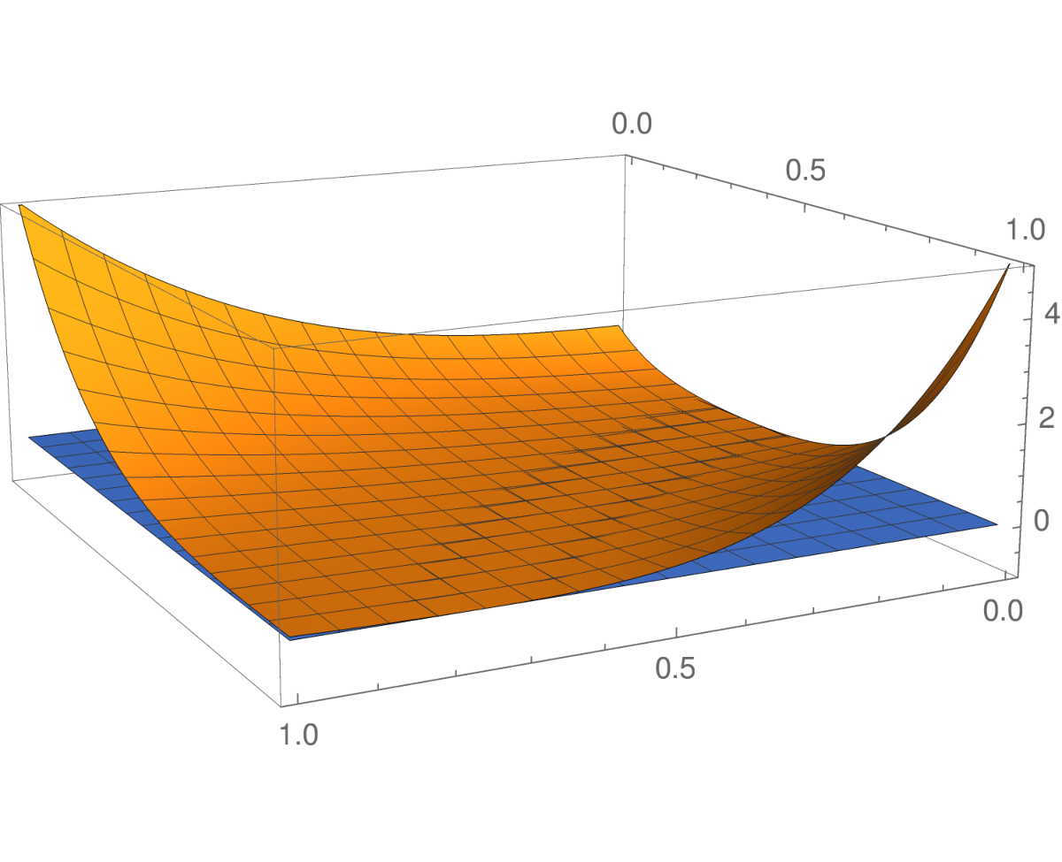
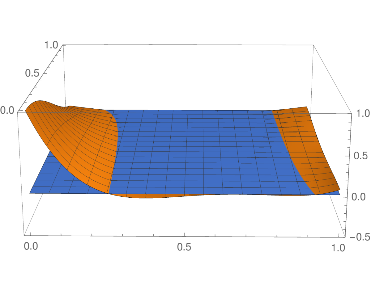
The system $(J_{(1,2)},H_{(s_{1},s_{2})})$ , $s_{1},s_{2}\in[0,1]$ , has exactly four critical points of rank $0$ , namely $\{(N,N),(N,S),(S,N),(S,S)\}$ . The points $(N,N)$ and $(S,S)$ are non-degenerate and of elliptic-elliptic type for all $s_{1},s_{2}\in[0,1]^{2}$ . The point $(N,S)$ is non-degenerate except when $(s_{1},s_{2})\in\gamma_{(N,S)}$ and the point $(S,N)$ is non-degenerate except when $(s_{1},s_{2})\in\gamma_{(S,N)}$ . In particular, for $s_{1},s_{2}\in\{0,1\}$ , all four points are elliptic-elliptic and for $s_{1}=s_{2}=\frac{1}{2}$ the points $(N,S)$ and $(S,N)$ are both focus-focus.

Proof.

Using Corollary 3.6, we study the behaviour of the discriminant $\triangle_{(\vec{s},\vec{e})}$ for the parameter values in question. If $(e_{1},e_{2})\in\{(1,1),(-1,-1)\}$ , we are in the chart around $(N,N)$ or $(S,S)$ and $\triangle_{(\vec{s},\vec{e})}$ is positive. Figure 6 shows a plot of the case $(e_{1},e_{2})=(1,1)$ . If $(e_{1},e_{2})\in\{(1,-1),(-1,1)\}$ , we are in the chart around $(N,S)$ or $(S,N)$ and $\triangle_{(\vec{s},\vec{e})}$ vanishes along two curves. Figure 7 shows a plot of the case $(e_{1},e_{2})=(1,-1)$ .

∎

Lemmas 4.1, 4.2, and 4.3 combine to form the following, which implies Theorem 1.2.

Theorem 4.4.

The system $(J_{(1,2)},H_{(s_{1},s_{2})})$ has the following properties:

1)

for all $s_{1},s_{2}\in[0,1]^{2}$ it is an integrable system such that, with the possible exception of $(N,S)$ and $(S,N)$ (depending on $s_{1}$ and $s_{2}$ ), all of the singular points are non-degenerate of type elliptic-elliptic or elliptic-regular;
2)

the points $(N,S)$ and $(S,N)$ are rank 0 singular points which transition between being of focus-focus, elliptic-elliptic, and degenerate as $(s_{1},s_{2})$ varies, and they are only degenerate on a set $\gamma\subset[0,1]^{2}$ which is the union of four smooth curves.

Thus, $(J_{(1,2)},H_{(s_{1},s_{2})})$ is a semitoric system for all $(s_{1},s_{2})\in[0,1]^{2}\setminus\gamma$ . In particular, if $(s_{1},s_{2})\in\{(0,0),(0,1),(1,0),(1,1)\}$ then $(J_{(1,2)},H_{(s_{1},s_{2})})$ is a semitoric system with no focus-focus points and the system $(J_{(1,2)},H_{(\frac{1}{2},\frac{1}{2})})$ is a semitoric system with exactly two focus-focus points.

Note that the set $\gamma$ is given in Equation (23) and is plotted in Figure 2.

4.1. A degenerate point

By Proposition 2.8 we know that for each $\vec{R}$ there exist some values of $s_{1},s_{2}\in[0,1]$ such that $(J_{\vec{R}},H_{(s_{1},s_{2})})$ is a degenerate system because the points $(N,S)$ and $(S,N)$ transition between being focus-focus and being elliptic-elliptic.

Example 4.5.

Assume that $s_{1}=s_{2}$ . Since $(J_{(1,2)},H_{(0,0)})$ and $(J_{(1,2)},H_{(1,1)})$ have no focus-focus points and $(J_{(1,2)},H_{\left(\frac{1}{2},\frac{1}{2}\right)})$ has focus-focus points at $(N,S)$ and $(S,N)$ there must exist at least two values of $s\in\ ]0,1[$ such that $(J_{(1,2)},H_{(s,s)})$ has a degenerate rank 0 point by Proposition 2.8. Plugging $t_{1}=(1-s)^{2}$ , $t_{2}=s^{2}$ , $t_{3}=2s(1-s)$ , $t_{4}=0$ , $e_{1}=-1$ , and $e_{2}=1$ into $\omega^{-1}_{p}d^{2}H$ in Equation 13 and taking the discriminant of the characteristic polynomial equal to zero gives exactly two solutions in the range $]0,1[$ . These solutions are $s_{+}$ and $s_{-}$ where

s_{\pm}=\frac{1}{31}\left(\pm 8\sqrt{5}+14\mp\sqrt{82\mp 24\sqrt{5}}\right)

and $s_{+}\approx 0.856953$ , $s_{-}\approx 0.250291$ . Since there must be at least two degenerate points and these are the only points for which $\omega^{-1}_{p}d^{2}H$ has less than four distinct eigenvalues we conclude that $(J_{(1,2)},H_{(s_{+},s_{+})})$ and $(J_{(1,2)},H_{(s_{-},s_{-})})$ have a degenerate point at $(S,N)$ .

Acknowledgments

The first author was partially supported by the Research Fund of the University of Antwerp and the second author is partially supported by an AMS-Simons travel grant. The second author is extremely grateful to the IHES for inviting him to visit in the summer of 2017, where some of the work for this project was completed. Additionally, both authors are thankful to Yohann Le Floch and Jaume Alonso Fernández for helpful discussions. Moreover, we thank Taras Skrypnyk for bringing the Gaudin model to our attention and for describing to us its relevance in mathematical physics.

References

[1] J. Alonso, H. Dullin and S. Hohloch, Taylor series and twisting-index invariants of coupled spin-oscillators, ArXiv:1712.06402.
[2] M. F. Atiyah, Convexity and commuting Hamiltonians, Bull. London Math. Soc., 14 (1982), 1–15.
[3] A. V. Bolsinov and A. T. Fomenko, Integrable Hamiltonian systems, Chapman & Hall/CRC, Boca Raton, FL, 2004, Geometry, topology, classification, Translated from the 1999 Russian original.
[4] P.-L. Buono, F. Laurent-Polz and J. Montaldi, Symmetric Hamiltonian bifurcations, in Geometric mechanics and symmetry, vol. 306 of London Math. Soc. Lecture Note Ser., Cambridge Univ. Press, Cambridge, 2005, 357–402, Based on lectures by Montaldi.
[5] R. Cushman and L. Bates, Global aspects of classical integrable systems, 2nd edition, Birkhäuser/Springer, Basel, 2015, URL https://doi.org/10.1007/978-3-0348-0918-4.
[6] R. Cushman and V. u Ngoc S., Sign of the monodromy for Liouville integrable systems, Ann. Henri Poincaré, 3 (2002), 883–894.
[7] T. Delzant, Hamiltoniens périodiques et images convexes de l’application moment, Bull. Soc. Math. France, 116 (1988), 315–339.
[8] H. Dullin and A. Pelayo, Generating hyperbolic singularities in semitoric systems via Hopf bifurcations, J. Nonlinear Sci., 26 (2016), 787–811.
[9] K. Efstathiou and N. Martynchuk, Monodromy of Hamiltonian systems with complexity 1 torus actions, J. Geom. Phys., 115 (2017), 104–115.
[10] L. H. Eliasson, Hamiltonian systems with Poisson commuting integrals, PhD thesis, University of Stockholm, 1984.
[11] M. Gaudin, Diagonalisation d’une classe d’hamiltoniens de spin, J. Phys. France, 37 (1976), 1087–1098, DOI: 10.1051/jphys:0197600370100108700.
[12] V. Guillemin and S. Sternberg, Convexity properties of the moment mapping, Invent. Math., 67 (1982), 491–513.
[13] S. Hohloch, S. Sabatini and D. Sepe, From compact semi-toric systems to Hamiltonian $S^{1}$ -spaces, Discrete Contin. Dyn. Syst., 35 (2015), 247–281.
[14] S. Hohloch, S. Sabatini, D. Sepe and M. Symington, Vertical almost toric systems, ArXiv:1706.09935.
[15] D. M. Kane, J. Palmer and A. Pelayo, Classifying toric and semitoric fans by lifting equations from $\rm{SL}_{2}(\mathbb{Z})$ , SIGMA Symmetry Integrability Geom. Methods Appl., 14 (2018), 016, 43 pages.
[16] D. M. Kane, J. Palmer and A. Pelayo, Minimal models of compact symplectic semitoric manifolds, J. Geom. Phys., 125 (2018), 49–74.
[17] Y. Karshon, Periodic Hamiltonian flows on four-dimensional manifolds, Mem. Amer. Math. Soc., 141 (1999), viii+71.
[18] Y. Le Floch and A. Pelayo, Symplectic geometry and spectral properties of classical and quantum coupled angular momenta, ArXiv:1607.05419.
[19] Y. Le Floch, A. Pelayo and S. Vũ Ngọc, Inverse spectral theory for semiclassical Jaynes-Cummings systems, Math. Ann., 364 (2016), 1393–1413.
[20] J. Marsden and T. Ratiu, Introduction to mechanics and symmetry, vol. 17 of Texts in Applied Mathematics, 2nd edition, Springer-Verlag, New York, 1999, URL https://doi.org/10.1007/978-0-387-21792-5, A basic exposition of classical mechanical systems.
[21] E. Miranda and N. T. Zung, Equivariant normal form for nondegenerate singular orbits of integrable Hamiltonian systems, Ann. Sci. École Norm. Sup. (4), 37 (2004), 819–839.
[22] J. Palmer, Moduli spaces of semitoric systems, J. Geom. Phys., 115 (2017), 191–217.
[23] A. Pelayo, Hamiltonian and symplectic symmetries: an introduction, Bull. Amer. Math. Soc. (N.S.), 54 (2017), 383–436.
[24] Á. Pelayo, T. Ratiu and S. Vũ Ngọc, The affine invariant of proper semitoric integrable systems, Nonlinearity, 30 (2017), 3993.
[25] A. Pelayo and S. Vũ Ngọc, Semitoric integrable systems on symplectic 4-manifolds, Invent. Math., 177 (2009), 571–597.
[26] A. Pelayo and S. Vũ Ngọc, Constructing integrable systems of semitoric type, Acta Math., 206 (2011), 93–125.
[27] A. Pelayo and S. Vũ Ngọc, Symplectic theory of completely integrable Hamiltonian systems, Bull. Amer. Math. Soc. (N.S.), 48 (2011), 409–455, URL https://doi.org/10.1090/S0273-0979-2011-01338-6.
[28] A. Pelayo and S. Vũ Ngọc, Hamiltonian dynamics and spectral theory for spin-oscillators, Comm. Math. Phys., 309 (2012), 123–154.
[29] M. Petrera, Integrable Extensions and Discretizations of Classical Gaudin Models, PhD thesis, Dipartimento di Fisica, Università degli Studi di Roma Tre, 2007.
[30] T. Ratiu, C. Wacheux and N. T. Zung, Convexity of singular affine structures and toric-focus integrable hamiltonian systems, ArXiv:1706.01093.
[31] D. A. Sadovskií and B. I. Zĥilinskií, Monodromy, diabolic points, and angular momentum coupling, Phys. Lett. A, 256 (1999), 235–244.
[32] M. Symington, Four dimensions from two in symplectic topology, in Topology and geometry of manifolds (Athens, GA, 2001), vol. 71 of Proc. Sympos. Pure Math., Amer. Math. Soc., Providence, RI, 2003, 153–208.
[33] S. Vũ Ngọc, On semi-global invariants for focus-focus singularities, Topology, 42 (2003), 365–380.
[34] S. Vũ Ngọc, Systèmes intégrables semi-classiques: du local au global, vol. 22 of Panoramas et Synthèses [Panoramas and Syntheses], Société Mathématique de France, Paris, 2006.
[35] S. Vũ Ngọc, Moment polytopes for symplectic manifolds with monodromy, Adv. Math., 208 (2007), 909–934.
[36] C. Wacheux, Systémes intégrables semi-toriques et polytopes moment, PhD thesis, Université de Rennes 1, 2013.
[37] J. Williamson, On the algebraic problem concerning the normal form of linear dynamical systems, Amer. J. Math., 58 (1936), 141–163.

A family of compact semitoric systems with two focus-focus singularitiesThanks: The first author was partially supported by the Research Fund of the University of Antwerp and the second author is partially supported by an AMS-Simons travel grant.

Abstract.

Key words and phrases:

1991 Mathematics Subject Classification

1. Introduction

Theorem 1.1.

Theorem 1.2.

Structure of the article:

Figures:

2. Fundamental definitions

2.1. Integrable systems and non-degenerate singular points

2.1.1. Integrable systems

2.1.2. Rank 0 singular points, i.e., fixed points

Definition 2.1.

Lemma 2.2 (Bolsinov &\& Fomenko [3]).

Sketch of proof.

2.1.3. Rank 1 singular points

Definition 2.3 (Bolsinov &\& Fomenko [3]).

Lemma 2.4.

Proof.

Corollary 2.5.

2.1.4. Classification of non-degenerate points

Theorem 2.6 (Eliasson [10], Miranda &\& Zung [21]).

Proposition 2.7 (Vũ Ngọc [34, Chapter 3]).

2.1.5. Degenerate points

Proposition 2.8.

Proof.

Remark 2.9.

2.2. Semitoric systems

Definition 2.10.

Theorem 2.11 (Classification by Pelayo &\& Vũ Ngọc [25, 26]).

2.3. The symplectic structure on 𝕊2{\mathbb{S}}^{2} and 𝕊2×𝕊2{\mathbb{S}}^{2}\times{\mathbb{S}}^{2}

2.4. Explicit examples of semitoric systems

Example 2.12 (Coupled angular momenta).

Example 2.13 (Coupled spin oscillator).

Remark 2.14.

3. A family of systems with two focus-focus points

3.1. The system

Theorem 3.1.

Remark 3.2.

Remark 3.3.

3.2. Rank 0 points and their nondegeneracy

Lemma 3.4.

Proof.

Lemma 3.5.

Proof.

Corollary 3.6.

Proposition 3.7 (Rank 0 Criterion).

Proof.

Corollary 3.8.

Proposition 3.9.

3.3. Rank 1 points

Lemma 3.10.

Proof.

Lemma 3.11.

Proof.

3.4. Integrability

Lemma 3.12.

Proof.

Proposition 3.13.

Proof.

3.5. Nondegeneracy of rank 1 points

Proposition 3.14 (Rank 1 Criterion).

Proof.

Corollary 3.15.

4. A linear combination of systems of toric type

Lemma 4.1.

Proof.

Lemma 4.2.

Proof.

Lemma 4.3.

Proof.

Theorem 4.4.

4.1. A degenerate point

Example 4.5.

Acknowledgments

References

Lemma 2.2 (Bolsinov $\&$ Fomenko [3]).

Definition 2.3 (Bolsinov $\&$ Fomenko [3]).

Theorem 2.6 (Eliasson [10], Miranda $\&$ Zung [21]).

Theorem 2.11 (Classification by Pelayo $\&$ Vũ Ngọc [25, 26]).

2.3. The symplectic structure on ${\mathbb{S}}^{2}$ and ${\mathbb{S}}^{2}\times{\mathbb{S}}^{2}$