Distribution of diameters for Erdős-Rényi random graphs
Abstract
We study the distribution of diameters of Erdős-Rényi random graphs with average connectivity . The diameter is the maximum among all shortest distances between pairs of nodes in a graph and an important quantity for all dynamic processes taking place on graphs. Here we study the distribution numerically for various values of , in the non-percolating and the percolating regime. Using large-deviations techniques, we are able to reach small probabilities like which allow us to obtain the distribution over basically the full range of the support, for graphs up to nodes. For values , our results are in good agreement with analytical results, proving the reliability of our numerical approach. For the distribution is more complex and no complete analytical results are available. For this parameter range, exhibits an inflection point, which we found to be related to a structural change of the graphs. For all values of , we determined the finite-size rate function and were able to extrapolate numerically to , indicating that the large deviation principle holds.
I Introduction
For each connected component of a network or a graph [1, 2, 3], the diameter is the maximum, over all pairs of component’s vertices , of the shortest-path distance . The diameter of a graph is the maximum over all components of . The diameter is an important measure of the network. It has a strong influence on, e.g., dynamical processes taking place on these networks, since it characterizes a typical long length scale for the transport of information. Examples for the importance of the diameter are rumour spreading [4], energy transport in electric grids [5] or oscillations in neural circuits [6]. Furthermore, for networks changing over time, the temporal evolution of the diameter can give important insights into the structure of the dynamics [7].
Not much is known about the behaviour of the diameter of random network ensembles. At least it is known that the average diameter for many ensembles grows logarithmically with the number of nodes [8]. Nevertheless, a full description, i.e., the probability distribution of network diameters over the instances of an random graph ensemble, has almost been obtained only in very limites cases, to the knowledge of the authors.
Thus, here we deal with the most fundamental and least-structured graph ensemble, which are Erdős-Rényi (ER) random graphs [9]. Let denote the number of vertices. Each realisation of an ER random graph is generated by iterating over the pairs of nodes and adding the edge with probability . Here we concentrate on the sparse case , being the average connectivity.
In the non-percolating phase , close to the percolation threshold , the distribution of diameters is described in theorem 11(iii) of Ref. [10]. The distribution is asymptotically () given by a Gumbel (extreme-value) distribution
| (1) |
Here, is the maximum of the distribution, which scales logarithmically with the number of nodes. is the Gumbel parameter describing the exponential behaviour for large values. It describes the variance, which is proportional to . In this limit, the Gumbel parameter as a function of the connectivity is given by
| (2) |
The fact that is connected to such an extreme-value distribution is intuitively clear: below the percolation threshold, each graph consists of a large number of trees, hence the diameter is obtained by maximising over these trees.
Note that Ref. [10] also contains results for general values of . Although they are given in a more complex and partially implicit form, they indicate that the asymptotic distribution is also the Gumbel distribution 1, with a parameter also given by 2.
Due to finite-size corrections, the distribution of diameters in finite-size graphs does not follow the Gumbel distribution. In earlier numerical studies of another problem, sequence alignments [11, 12, 13], the data was well fitted by “modifying” the Gumbel distribution by a Gaussian factor:
| (3) |
where is given through the normalisation . This distribution will be used in our analysis.
The probabilities for values of which deviate from the typical size are often exponentially small in . Hence, one uses the concept of the large-deviation rate function [14, 15] by writing
| (4) |
Note that the normalisation is part of the factor. One says that the large-deviation principle holds if, loosely speaking, the empirical rate function
| (5) |
converges to for . Due to the logarithm the normalisation and the sub-leading term of become an additive contribution to , which go to zero for .
In the present work, we study numerically the distribution of diameters of ER random graphs in the sparse regime . Using a large-deviation technique which is based on studying a biased ensemble characterised by a finite temperature-like parameter, see Sec. II, we are able to obtain the distributions over almost the full ranges of the support, down to very small probabilities like . For the non-percolating regime , we compare our numerical results to the available analytical results and find a good agreement. In particular we find that the asymptotic result of a suitably scaled Gumbel distribution, modified by a Gaussian finite-size correction, is compatible for all values with our results. Also, we find the dependence (2) of the Gumbel parameter as a function of , for . This confirms the validity of our approach.
We are also able to obtain numerically for where no exact result is available to our knowledge. Here we find that the distributions exhibit an inflection point. This leads to a first-order transition in our finite-temperature ensemble and makes the numerical determination of the distribution much harder.
Nevertheless, for all values of , we determined the rate functions for various numbers of nodes and obtained, where necessary, the limiting rate function via extrapolation. In all cases we observed a good convergence, indicating that the large-deviation principle seems to hold.
II Simulation and reweighting method
We are interested in determining the distribution for the diameter of an ensemble of random graphs. The distribution can be obtained in principle for any graph ensemble, here we apply it to ER random graphs. Simple sampling is straightforward: One generates a certain number of graph samples and obtains for each sample . This means each graph will appear with its natural ensemble probability . The probability that the graph has diameter is given by
| (6) |
Therefore, by calculating a histogram of the values for , an estimation for is obtained. Nevertheless, with this simple sampling, can only be measured in a regime where is relatively large, about . Unfortunately, the distribution usually decreases very quickly, e.g., exponentially in the system size when moving away from its typical (peak) value, like in Eq. (4) This means that even for moderate system sizes , the distribution will be unaccessible through this method, on almost its complete support.
II.1 Markov-chain Monte Carlo approach
To estimate for a much larger range of diameters, a different importance sampling approach is used [11, 16]. For self-containedness, the method is outlined subsequently. The basic idea is to generate random graphs with a probability that includes an additional Boltzmann factor , being a “temperature” parameter, in the following manner: A standard Markov-chain MC simulation [17, 18] is performed, where the current state at “time” is given by an instance of a graph . Here the Metropolis-Hastings algorithm [19] is applied as follows: at each step a candidate graph is created from the current graph . One then computes the diameter of the candidate graph, . To complete a step of the Metropolis-Hastings algorithm, the candidate graph is accepted, () with the Metropolis probability
| (7) |
Otherwise the current graph is kept ().
Here, the genreation of is done using the following local update rule: A node of the current graph is selected randomly, with uniform weight , and all adjacent edges are deleted. Next, the node is reconnected again: for all other nodes the corresponding edge is added with a probability (and not added with probability ), which corresponds to its contribution to the natural weight of an ER graph.
By construction, the algorithm fulfils detailed balance. Clearly the algorithm is also ergodic, since within steps, each possible graph may be constructed. Thus, in the limit of infinitely long Markov chains, the distribution of graphs will follow the probability
| (8) |
where is the a priori unknown normalisation factor. Note that for all candidate graphs will be accepted and the distribution of graphs will follow the original ER weights.
II.2 Obtaining the distribution
The probability to measure at any temperature is given by
| (9) |
Hence, the target distribution can be estimated, up to a normalisation constant , from sampling at finite temperatures . For each temperature, a specific range of the distribution will be sampled: Using a positive temperature allows to sample the region of a distribution left to its peak (values of the diameter smaller than the typical value). Since is only an artificial resampling parameter, also negative temperatures are feasible, which therefore allow us to access the right tail of . In both cases, temperatures of large absolute value will cause a sampling of the distribution close to its typical value, while temperatures of small absolute value are used to access the tails of the distribution. Hence one chooses a suitable set of temperatures with and being the number of negative and positive temperatures, respectively. A good choice of the temperatures is such that the resulting histograms of neighbouring temperatures overlap sufficiently. This allows to “glue” the histograms together, see next paragraph. By obtaining the distributions , …, , such that is “covered” as much as possible, one can measure over a large range, possibly on its full support. The range where the distribution can be obtained may be limited, e.g., when the MC simulations at certain temperatures do not equilibrate. This happens usually for small absolute values , where the system might also have a glassy behaviour. Another difficult case is when is not concave: then a first order transition will appear [16] as a function of , which might prevent one from obtaining in some regions of the support for large systems.
The normalisation constants can easily be computed, e.g., by including a histogram generated from simple sampling, which corresponds to the temperature . Using suitably chosen temperatures , , one measures histograms which overlap with the simple sampling histogram on its left and right border, respectively. Then the corresponding relative normalisation constants can be obtained by the requirement that, after rescaling the histograms according to (9), they must agree in the overlapping regions with the simple sampling histogram within error bars. This means, the histograms are “glued” together. In the same manner, the range of covered values can be extended iteratively to the left and to the right by choosing additional suitable temperatures and gluing the resulting histograms one to the other. The histogram obtained finally can be normalised (with constant ), such that the probabilities sum up to one. This also yields the actual normalisation constants from Eq. (9). Note that one could also not only glue together neighbouring histograms, but use for each bin value all data which is available, as it is done, e.g., within the multi-histogram approach by Ferrenberg and Swendsen [20]. For the present case, it was easy to obtain good data statistics such that it was sufficient to use the histograms just pairwise.
A pedagogical explanation of the gluing process and examples of this procedure can be found in Ref. [21].
II.3 Equilibration
In order to obtain the correct result, the MC simulations must be equilibrated. In our case, there is an easy test that can indicate when equilibration has not been reached. One can run two simulations starting with two different initial graphs , respectively:
- •
a graph which is arranged in a line, i.e., it has a linear structure with nodes and edges. The diameter of this graph is .
- •
a complete graph, which contains all possible edges. For this graph the diameter is one.
For each of these two different initial conditions, the evolution of will approach the equilibrium range of values from two different extremes, which allows for a simple equilibration test: if the measured values of disagree within the range of fluctuation, equilibration is not achieved. We shall assume that, conversely, if the measured values of agree, then equilibration has been obtained.
Note that one can also use generalised ensemble methods like the Multicanonical method [22] or the Wang-Landau approach [23], in particular when a first order transition as function of appears, to obtain the distribution . While these methods in principle do not require to perform independent simulations at different values for the temperatures, it turns out that for larger system sizes, one still has to perform multiple simulations because one has to split the interval of interest into smaller overlapping sub intervals, to make the simulation feasible. Here, the Wang-Landau algorithm was used only for the case of , where the temperature-based approach did not work well, see below. For other values of , it turned out to be much easier to guide the simulations to the regions of interest, e.g., where data is missing using the so-far-obtained data, and to monitor the equilibration process, using the finite-temperature approach.
III Results
We have numerically determined the distribution of diameters for ER random graphs for different connectivities below, above and at the percolation threshold .
III.1 Connectivity
We start with the non-percolating regime, where we can compare with exact asymptotic results [10]. In Fig. 1, is shown at for three different graph sizes. Using the approach explained in the last section, probabilities as small as are easily accessible. In the log-log plot, clearly a curvature in the data is visible for large values of the diameter, which could be partially due to strong finite-size corrections. We have fitted the data to a modified Gumbel distribution Eq. (3) and obtained good fit qualities. We studied the strength of the Gaussian correction, see inset of Fig. 1. One observes a clear power-law behaviour. Hence, the numerical data supports that asymptotically the full distribution becomes Gumbel or Gumbel-like below the percolation threshold.

We have studied the behaviour in the non-percolating phase for various values of the connectivity and different system sizes, see Fig. 2 for . Each time we observe qualitatively the same convergence to a Gumbel distribution.

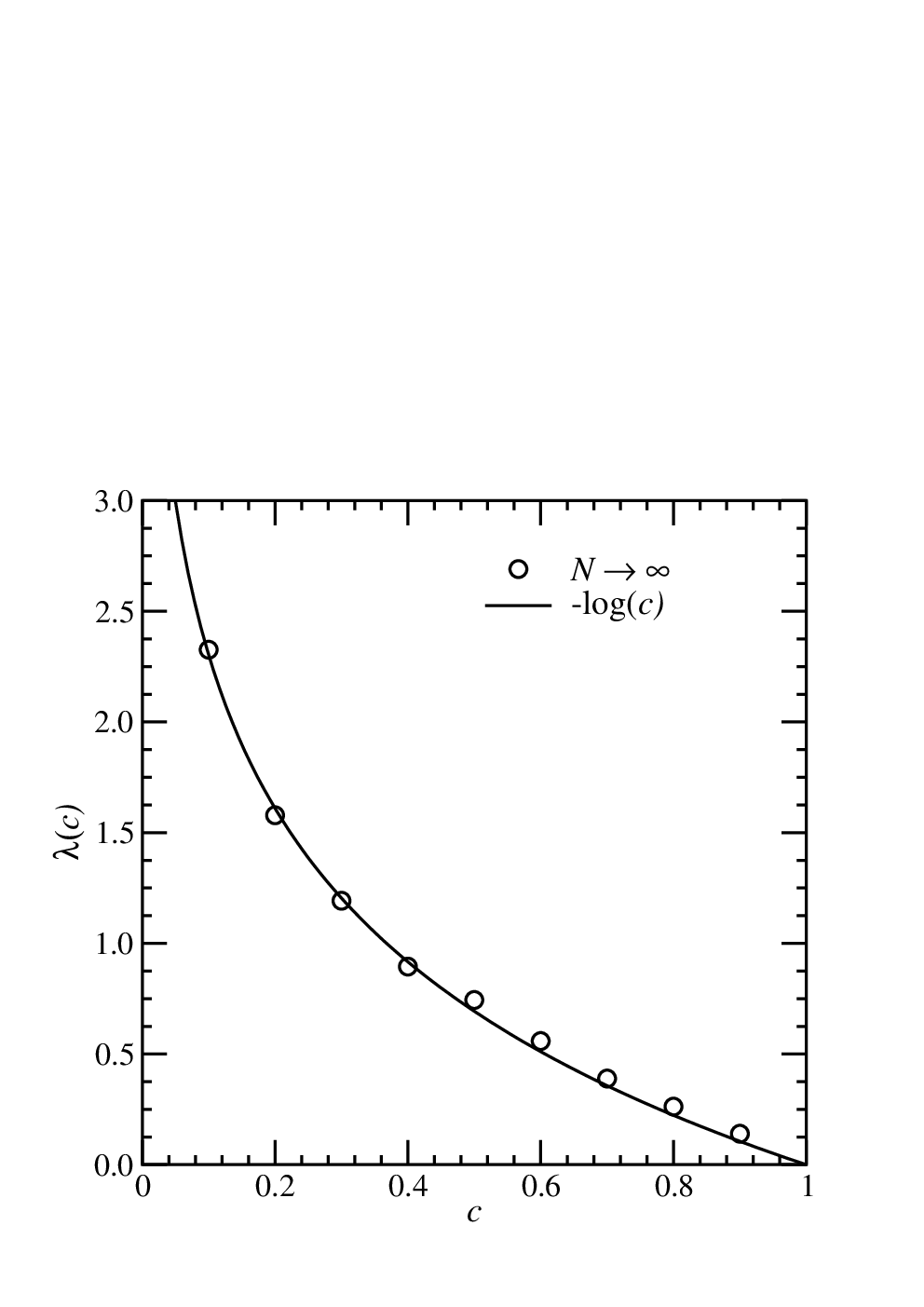
From the fits, for each value of the connectivity and each system size , a value of is obtained. To extrapolate the dependence of the Gumbel parameter to large graph sizes, the following heuristic dependence, inspired by standard finite-size scaling [24, 25] was applied:
| (10) |
The inset of Fig. 2 shows the behaviour of together with the fit as function of graph size . The resulting values for as a function of the connectivity are shown in Fig. 3 together with the asymptotic result Eq. (2), yielding a nice agreement. This shows that indeed the numerical approach allows to reliably study the distribution of diameters for finite sizes and to extrapolate to large graphs.
Nevertheless, the scaling of the Gaussian correction parameter is basically close to , hence when looking at the data for the rescaled diameter , the size-dependence exactly drops out. Hence, the rate function Eq. (5) as a function of is studied next, as displayed in Fig. 4. The data collapse is good, which means that even for small system sizes the rate function is well converged. This means that the distribution of diameters can indeed be described well by a rate function, hence the large-deviation principle [26, 14] holds. This makes it a bit more likely that this model is accessible to the mathematical tool of the large-deviation theory. Note that due to the curvature of the rate function, the Gumbel distribution is not visible when inspecting the result on the scale, which makes the most-important finite-size contribution drop out. Only when one looks at the data at fixed values , the convergence to a Gumbel is a meaningful statement. A similar result has been observed previously for the distribution of scores of sequence alignment [13].

III.2 Connectivity
The results for the non-percolating phase gave us confidence that the numerical method allows us to turn our attention to cases, where no exact results for the full distribution are available. In Fig. 5, the distribution of diameters is shown right at the percolation transition . Here, the random graph consists of a large extensive tree plus small components and no Gumbel distribution is expected, since .
Nevertheless, it is still possible to fit the finite-size data to the modified Gumbel distribution, see Fig. 5, since any finite-size graph for cannot be distinguished from the case close to 1. For example, fitting the case to Eq. (3) resulted in
The fit matches the data well, also for other systems sizes. Nevertheless, when studying the dependence of on the system size, a convergence towards zero seems most likely, see inset of Fig. 5. In the double-logarithmic plot the data appears to be compatible with a straight line, meaning a power-law decrease, and maybe even a faster decrease. We verified this by fitting according to Eq. (10), where we obtained a negative value for for with an error bar of almost the same size, showing that indeed the distribution differs from the Gumbel distribution for .
This can also be seen from studying the large-deviation rate function , see inset of Fig. 4 where also an upward-bending function is seen, as for the case .

III.3 Connectivity
In the percolating phase , the numerical result show that in the artificial finite-temperature ensemble there appears to be a 1st order phase transition as a function of the temperature, similarily to the distribution of the size of the largest component [16]. To visualise this, we here only show an example of a MC time series for the diameter, see Fig. 6. Clearly the diameter oscillates between two distinct regimes, showing the coexistence of two “phases’ with small and large diameter, respectively. This corresponds at this temperature to a distribution of diameters with two peaks.

The data in Fig. 6 of the size of the largest component and the size of the largest biconnected component suggest that the system oscillates between two states. When the diameter is small, around 30 here, the largest biconnected component is large, it contains about 200 nodes. On the other hand, when the diameter is large, about 130, the largest biconnected component has a size of only about 30. Nevertheless, the size of the largest components changes only a little bit. This we interpret in the following way.
There is always one large line-like object present and a tightly (bi-) connected cluster, see Fig. 7. As we have verified explicitly in our numerical data, the tightly connected cluster typically has a small diameter while the line-like object has a large diameter. In one state, the line-like object is connected to the tightly connected cluster only at few nodes or not at all. Hence, the diameter path is basically along the line-like object and the diameter is large. In the other state, the line-like object is connected to the tightly-connected cluster at several, distant points, such that the diameter path makes a shortcut. Thus, the diameter is small and the biconnected component relatively large. Our measurements showed that although the diameters of the two states differ strongly, the number of edges differ only slightly (not shown here). This allows for a quick transition between the two states. Note that in the mathematical literature [27] for a logarithmically growing connectivity for diluted ER random graphs, the diameter is concentrated around a finite number (larger than one) of values. This might be related to the observed oscillations of the diameter.

The existence of an inflection points translates into the existence of a first-order transition in the finite temperature ensemble with some criticial temperature . This leads to a bimodal structure of exhibiting a very small probability in the region between the two peaks. Hence, concerning the numerical effort, obtaining the full distribution becomes difficult, in particular for large graphs, because the intermediate region for values of between the two peaks of is rarely or even not at all sampled.

Therefore, for the case , only system sizes up to could be equilibrated deep into the large-diameter regime (corresponding to negative temperatures with small absolute value). The first-order nature of the transition, i.e., the two-peak structure of the distributions of the diameter at finite-temperature close to the transition temperature, becomes visible by a “dip” in the distribution of diameters for .
The dip is more pronounced when going to larger connectivities. This can be seen in Fig. 9, where the large-deviation rate function is displayed for for different system sizes. Here, the Wang-Landau approach was used, which allowed us to sample the region of the dip much better.

In Fig. 9 the corresponding rate function is shown. Here, in particular for small values of , stronger finite size effects are visible. Thus, we have considered the functions at various fixed rations and performed an extrapolation via fitting
| (11) |
where and are fitting parameters which are determined for each considered value of separately, i.e., point-wise. An example of the extrapolation is shown in Fig. 9, together with the extrapolated values . For large values of , above 0.5, the small finite size effects are small, while for small values of the extrapolated function differs slightly from the results for finite values of . The change from a concave to a convex function near is well visible. A similar qualitative behaviour has been found previously for the rate function for the distribution of the size of the largest component for ER random graphs.
IV Summary
We have studied the distribution of the diameter for dilute ER random graphs with connectivities . Using large-deviations simulations techniques, we were able to obtain the distributions over large ranges of the support. In the non-percolating region of small connectivities , the distributions are concave and can be well fitted to the Gumbel distributions with a Gaussian correction. The extrapolated parameter of the Gumbel distribution agrees well with mathematical results. In the percolating regime the distribution of the diameters is not available. Within the numerical result, we observed a change from concave to convex behaviour, thus a more complex distribution. Nevertheless, for all values of we studied, we were able to obtain and extrapolate the rate function. This means that the distribution of diameters follows the large deviation principle.
Since the diameter is of importance for many physical processes taking place on networks, it would be interesting to obtain the distribution over a large range of the support for other graph ensembles, like scale free graphs. The results obtained in the present work show that this should in principle be possible.
Acknowledgements
We thank Charlotte J. Beelen for many valuable discussions and a critical reading the manuscript. This project was supported by the German Humboldt foundation. MM thanks the University of Oldenburg for the hospitality. AKH is grateful for the hospitality and the financial support of the LPTMPS, Université Paris-Sud, were he spent part of his sabbatical. The simulations were performed on the HERO cluster of the University of Oldenburg jointly funded by the DFG (INST 184/108-1 FUGG) and the ministry of Science and Culture (MWK) of the Lower Saxony State.
References
- [1] R. Cohen and S. Havlin, Complex networks: structure, robustness and function (Cambridge Univ. Press, 2010).
- [2] M. Newman, Networks: an Introduction (Oxford University Press, 2010).
- [3] E. Estrada, The structure of complex networks: theory and applications (Oxford University Press, 2011).
- [4] B. Doerr, M. Fouz, and T. Friedrich, Commun. ACM 55, 70 (2012), ISSN 0001-0782.
- [5] A. K. Hartmann, Eur. Phys. J. B 87, 114 (2014), ISSN 1434-6028.
- [6] A. Goldental, R. Vardi, S. Sardi, P. Sabo, and I. Kanter, Front. Neur. Circ. 9, 65 (2015), ISSN 1662-5110.
- [7] B. Blonder, T. W. Wey, A. Dornhaus, R. James, and A. Sih, Meth. Ecol. Evol. 3, 958 (2012), ISSN 2041-210X.
- [8] R. Albert and A.-L. Barabási, Rev. Mod. Phys. 74, 47 (2002).
- [9] P. Erdős and A. Rényi, Publ. Math. Inst. Hungar. Acad. Sci. 5, 17 (1960).
- [10] T. Łuczak, Rand. Struct. Alg. 13, 485 (1998), ISSN 1098-2418.
- [11] A. K. Hartmann, Phys. Rev. E 65, 056102 (2002).
- [12] S. Wolfsheimer, B. Burghardt, and A. K. Hartmann, Alg. Mol. Biol. 2, 9 (2007).
- [13] L. Newberg, J. Comp. Biol. 15, 1187 (2008).
- [14] F. den Hollander, Large Deviations (American Mathematical Society, Providence, 2000).
- [15] H. Touchette, Phys. Rep. 478, 1 (2009), ISSN 0370-1573.
- [16] A. K. Hartmann, Eur. Phys. J. B 84, 627 (2011).
- [17] M. E. J. Newman and G. T. Barkema, Monte Carlo Methods in Statistical Physics (Clarendon Press, Oxford, 1999).
- [18] D. P. Landau and K. Binder, Monte Carlo Simulations in Statistical Physics (Cambridge University Press, Cambridge, 2000).
- [19] N. Metropolis, A. W. Rosenbluth, M. N. Rosenbluth, A. Teller, and E. Teller, J. Chem. Phys. 21, 1087 (1953).
- [20] A. M. Ferrenberg and R. H. Swendsen, Phys. Rev. Lett. 63, 1195 (1989).
- [21] A. K. Hartmann, in New Optimization Algorithms in Physics, edited by A. K. Hartmann and H. Rieger (Whiley-VCH, Weinheim, 2004), p. 253.
- [22] B. A. Berg and T. Neuhaus, Phys. Rev. Lett. 68, 9 (1992).
- [23] F. Wang and D. P. Landau, Phys. Rev. Lett. 86, 2050 (2001).
- [24] J. Cardy, Finite-size Scaling (Elsevier, Amsterdam, 1988).
- [25] N. Goldenfeld, Lectures on phase transitions and the renormalization group (Addison-Wesely, Reading (MA), 1992).
- [26] A. Dembo and O. Zeitouni, Large Deviations Techniques and Applications (Springer, Berlin, 2010).
- [27] F. Chung and L. Lu, Adv. Appl. Math. 26, 257 (2001), ISSN 0196-8858.