interaction from lattice QCD
and its application to hypernuclei
Abstract
The interaction between and a nucleon () is investigated by employing the HAL QCD method in the (2+1)-flavor lattice QCD on a volume at MeV. We study the central potential in channel as well as central and tensor potentials in channel, and find that the tensor potential for is negligibly weak and central potentials in both and channels are almost identical with each other except at short distances. Phase shifts and scattering lengths calculated with these potentials show that the interaction of system is attractive and has a similar strength in and channels at low energies (i.e. the kinetic energy less than about MeV). While the attractions are not strong enough to form two-body bound states, our results lead to a possibility to form hypernuclei for sufficiently large atomic numbers (). To demonstrate this, we derive a single-folding potential for hypernuclei from the -nucleon potential obtained in lattice QCD, and find that hypernuclei can exist for with the binding energies of a few MeV. We also estimate the Coulomb effect for the hypernuclei.
Keywords:
Charmed baryon interaction , Charmed hypernuclei , Lattice QCD1 Introduction
The investigation of baryon-baryon interactions is one of the most important subjects to understand properties of hadronic matter. The low-energy nucleon-nucleon () interaction has been severely constrained by the scattering data and the properties of finite nuclei [1]. The hyperon-nucleon () and hyperon-hyperon () interactions have also been investigated phenomenologically to reproduce the properties of hypernuclei and hyperon-nucleon scattering data [2]. Such phenomenological interactions are then used to study yet unknown nuclei and also the neutron star interiors.
As a natural extension, it is interesting to investigate charmed hypernuclei, as initiated in Ref. [3] just after the discovery of the baryon. Including charm quarks, the one-boson-exchange potential (OBEP) model for the was constructed [4], where the couplings are determined by assuming the flavor , which is an extension of the flavor for the interaction. The possibility of both and nuclear bound states was predicted for heavy nuclei [3]. Further studies were carried out in [5, 6, 7]: Based on flavor symmetry, the authors made a comparison between the hypernuclei and the hypernuclei. Although the depth of the effective potential for in the G-matrix calculation is about of that for , they found that the number of bound states in hypernuclei is larger than that in hypernuclei due to its heavy mass.
However, the charm quark is much heavier than other three quarks (up, down, strange), so that the flavor may not give a good description of the interaction. Therefore, Ref. [8] has investigated interaction with the OBEP model based on the heavy quark effective theory, where the coupled channel system is considered. It was then found that interaction is strong enough to form a 2-body bound state due to effects of these channel couplings, but the results are rather sensitive to the model parameters. Studies within a framework of the constituent quark model [9, 10, 11, 12] have also been attempted to extract the interaction. In Ref. [13, 14], the authors have estimated the single particle energy for baryon in several nuclei by using the quark-meson coupling model, and they claim that hypernuclei are likely to be formed.
The aim of the present paper is to shed a new light on the problem of the interaction from first-principles lattice QCD simulations. For this purpose, the HAL QCD method to analyze the hadron-hadron interactions on the lattice [15, 16, 17] is most suitable. The method has already been applied to various hadron-hadron systems [18, 19, 20, 21, 22, 23] and to hadronic matter [24]. Advantages of this method in the context of the present paper are as follows: (i) Applications to the charmed systems are straightforward, (ii) no phenomenological parameters are involved since it is based on first-principles QCD simulations, and (iii) the resultant potential is faithful to the QCD S-matrix below the inelastic threshold, so that we can correctly calculate the elastic scattering phase shift.
This paper is organized as follows. In section 2, we present a brief description of the HAL QCD method for the system. The numerical setup for this work is summarized in section 3. In section 4, we show our numerical results of the potentials in both and channels. We also discuss properties of the interaction through phase shifts and scattering lengths calculated by our potentials. In section 5, we employ the single-folding potential to investigate hypernuclei. Summary and conclusions are presented in section 6.
2 HAL QCD method for system
In this section, we discuss the HAL QCD method [15] to be applied to the system. We start with the equal-time Nambu-Bethe-Salpeter (NBS) wave function in the center-of-mass (CM) frame of two baryons at Euclidean time ;
| (1) |
where are the spinor indices, and denotes a local interpolating operator for a baryon . The state stands for an energy eigenstate of a two baryon system. Here the total energy is denoted by with the baryon masses and , and the relative momentum . We employ the local interpolating operators for a nucleon and as
| (2) |
where , and are color indices. is the charge conjugation matrix defined by , and stands for quark operators for up-, down- and charm-quarks, respectively. Flavor structures of a nucleon and are given by
| (3) | |||||
| (4) |
In the asymptotic region (), the NBS wave function satisfies the Helmholtz equation and its asymptotic behavior for a given orbital angular momentum and total spin is denoted as
| (5) |
where the “scattering phase shift" is determined from the unitarity of the S-matrix in QCD [16, 17]. From the NBS wave function, the potential which reproduces the scattering phase shift is defined through the Schrödinger equation as
| (6) |
where with the reduced mass , and is a kinetic energy of the two baryon system in the CM frame. In this definition, the non-local potential is energy-independent below the inelastic threshold [16, 17]. In order to handle the non-locality of the potential, we introduce the derivative expansion as [25]
| (7) |
where is then expanded in terms of . For example, the leading order of the derivative expansion is given by
| (8) |
where is the Pauli matrix acting on the spin index of the -th baryon. The local potentials , and , which give the spin-independent force, the spin-spin force and the tensor force, are commonly used in nuclear physics. The convergence of the derivative expansion can be checked e.g. by changing the energy. For example, the leading order approximation is found to be accurate for MeV in the case of the scattering in quenched QCD with MeV [26].
In lattice QCD, the NBS wave functions can be extracted from the baryon four-point correlation function given by
| (9) |
where is the source operator which creates two baryon states with the total angular momentum and the parity . Inserting a complete set between the two-baryon operator and the source operator in the Eq. (9), we obtain
| (10) | |||||
with constant , where stands for an elastic scattering state with the energy of , and the ellipses represent contributions from inelastic states.
2.1 Source operator
In this work, we choose a wall source at defined by
| (11) |
where is the projection operator to the total angular momentum and the parity . Here is obtained by replacing the local quark operator in the with the wall quark operator given by
| (12) |
with the Coulomb gauge fixing at . Since the orbital angular momentum of the wall source is fixed to , the source with fixed total angular momentum are obtained by the spin projection of the source. In the case of the system, which has the total spin or , the wall source operator with the spin projection to or creates the system with or , respectively.
2.2 Time dependent HAL QCD method
In principle, the baryon four-point correlation function is dominated by the NBS wave function of the ground state in the large time separation (Eq. (10)). In practice, however, it is difficult to realize the ground state domination since cannot be taken large enough due to statistical noises of the baryon four-point correlation function [27, 28, 29, 30]. This difficulty was overcome by the time-dependent HAL QCD method [31] as follows. Let us consider the normalized baryon four-point correlation function from Eq. (9) as
| (13) | |||||
where , which satisfies
| (14) |
where . Using the above relation and the Schrödinger equation in Eq. (6), we obtain
| (15) |
for a moderately large , where contributions from the inelastic states can be neglected. Although the higher order terms in Eq. (14) can be calculated by corresponding time derivative, those contributions turn out to be numerically negligible in the present lattice setup. The effects of higher derivative terms and the contribution from inelastic states are regarded as the systematic errors and estimated by the time dependence of scattering observables. It is noted that Eq. (15) becomes exact for .
3 Lattice setup
For numerical simulations, we employ the (2+1)-flavor full QCD configurations generated by PACS-CS Collaboration [32] with the renormalization-group improved Iwasaki gluon action and a nonperturbatively improved Wilson-clover quark action at on a lattice. The corresponding lattice spacing is fm and physical lattice size is fm.
In order to see the quark mass dependence of the potentials, we employ three ensembles of gauge configurations. The hopping parameters of these ensembles are (Ensemble 1), (Ensemble 2), (Ensemble 3) for , -quarks while (Each ensemble) for the -quark. For the charm quark, we employ the relativistic heavy quark (RHQ) action [33] to avoid the leading and the next-to-leading discretization errors due to the charm quark mass . We use the RHQ parameters determined in Ref. [34] so as to reproduce the experimental value of the mass and the relativistic dispersion relation for the charmonium in spin-averaged state. Note that charm-quark loops are not considered in the present paper. The effects of charm loops for charmed baryons are expected to be small as studied e.g. in Ref. [35, 36]. Nevertheless, the effects to the interaction is an interesting open question to be investigated in the future.
We calculate quark propagators with the periodic boundary condition for the spatial directions, while the Dirichlet boundary condition is imposed on the temporal direction at the time-slice . Correlation functions for are calculated using the unified contraction algorithm [37]. In order to increase the statistics, we take an average over forward and backward propagations in time. Furthermore, we take 64 different time-slices for each configuration as the wall source location. The total statistics of each ensemble are given in Table 1.
| # of gauge configs. | # of sources | [MeV] | [MeV] | |
|---|---|---|---|---|
| Ensemble 1 | 399 | 64 2 | 702(2) | 1581(6) |
| Ensemble 2 | 400 | 64 2 | 570(1) | 1399(9) |
| Ensemble 3 | 450 | 64 2 | 412(2) | 1215(9) |
For all analyses in this study, we employ the jackknife method to estimate statistical errors. The bin-size of the jackknife samples is taken to 57, 40 and 45 for the Ensemble 1, 2 and 3, respectively. We confirm that change of bin-size does not affect the errors for hadron masses as well as the errors for potentials and phase shifts.
Various hadron masses calculated in this work are summarized in Table 2.
| Ensemble 1 | Ensemble 2 | Ensemble 3 | |
|---|---|---|---|
| 702(2) | 570(1) | 412(2) | |
| 789(2) | 713(1) | 637(2) | |
| 1999(1) | 1949(2) | 1904(2) | |
| 1581(6) | 1399(9) | 1215(9) | |
| 1642(6) | 1493(7) | 1342(6) | |
| 1657(6) | 1522(8) | 1395(9) | |
| 1881(11) | 1749(16) | 1631(28) | |
| 2685(3) | 2555(5) | 2434(6) | |
| 2780(5) | 2674(7) | 2575(9) | |
| 2866(5) | 2763(7) | 2661(10) |
4 Numerical results
4.1 central potentials in channel
We first discuss the central potential for the -wave spin-singlet system. In order to obtain the potential, we use the -correlator with the wall source defined in Eq. (13), which is further projected to the channel as
| (16) |
where and are projection operators to the total spin and the orbital angular momentum , respectively11 1 These projections are redundant since the state allows only the channel.. On the lattice, we employ the cubic transformation group for the projection of the orbital angular momentum as
| (17) |
where is one of 24 elements in . This projection picks up an representation of . By using the -correlator in the channel, we extract the central potential through Eq. (15). Since and for the state, we have
| (18) | |||||
for the moderately large .

Fig. 1 shows the central potential in the channel for each ensemble. The potential is calculated at (Ensemble 1: 700 MeV), (Ensemble 2: 570 MeV) and (Ensemble 3: 410 MeV). We find a repulsive core at short distances ( fm) and an attractive pocket at intermediate distances ( fm) in the potential. We also observe that the height of the repulsive core increases and the minimum of the attractive pocket shifts outward, as , quark masses decrease. A variation of the repulsive core against , quark masses may be explained by the fact that the color magnetic interaction is proportional to the inverse of the constituent quark mass [38]. We notice that the attraction of the potential seems weaker than that of the potential in Ref. [39].

In order to check the stability of the potential against the time separations , we plot the time dependence of the central potential in the channel at several different time separation in Fig. 2. In Fig. 2 (a), we find that the potential exhibits non-negligible time dependence for . The potential, however, becomes stable at larger time, , as shown in Fig. 2 (b). This observation suggests that contributions from inelastic states are negligible at , so that we take the potential at for 700 MeV case. For 570 and 410 MeV cases, we find that potentials are stable within the statistical errors at earlier time slices () as shown in Fig. 2 (c,d). This implies that the contaminations from inelastic states are more suppressed as quark masses are decreased: In fact, the excitation energy to the lowest inelastic state () becomes larger for lighter quark masses. Another possible reason is that the statistical errors at fixed become larger for lighter quark masses and tend to dominate the total error budget compared to the systematic errors from inelastic states. Under these considerations, we take at 570 MeV and at 410 MeV in the following analyses.
We then calculate physical observables such as scattering phase shifts in the channel from the potential. For this purpose, we fit the potential data with the functional form given by
| (19) |
Table 3 shows fit-parameters for the central potential in the channel on each ensemble. Using data at fm, we achieve .
| channel | channel | |||||
|---|---|---|---|---|---|---|
| 702(2) MeV | 570(1) MeV | 412(2) MeV | 702(2) MeV | 570(1) MeV | 412(2) MeV | |
| 1090(36) | 1266(20) | 1520(24) | 458.1(53.8) | 682.6(13.4) | 853.8(17.2) | |
| 0.09761(233) | 0.09912(112) | 0.1121(11) | 0.09296(835) | 0.1061(138) | 0.1183(16) | |
| 854.4(50.2) | 892.5(27.3) | 712.4(12.8) | 761.6(71.8) | 631.0(17.5) | 569.2(11.2) | |
| 0.4384(45) | 0.4670(36) | 0.6808(51) | 0.4208(59) | 0.4886(32) | 0.6898(56) | |
| -18637(5796) | -29804(6231) | -45479(4116) | -71142(38550) | -19158(3687) | -40798(3994) | |
| 1.566(154) | 1.182(84) | 0.6635(229) | 0.8462(1626) | 1.163(77) | 0.6144(221) | |
| 3.493(122) | 3.308(74) | 2.367(25) | 3.971(164) | 3.071(66) | 2.331(27) |
We solve the Schrödinger equation with the fitted potential in the infinite volume and extract its phase shifts from the asymptotic behavior of the wave function. Finally, the -wave scattering length is calculated as
| (20) |
Here we employ the particle physics convention for the definition of scattering length which has opposite sign from the historical sign convention of the baryon-baryon interaction.

| channel | channel | |
|---|---|---|
| 412(2) MeV | 0.49 (18) (11) fm | 0.51 (20) ( 9) fm |
| 570(1) MeV | 0.24 (13) ( 3) fm | 0.29 (16) ( 9) fm |
| 702(2) MeV | 0.13 (11) (11) fm | 0.17 (10) (12) fm |
Fig. 3 show the phase shift and the scattering length for the system in the channel for each ensemble, and the numerical values of the scattering length are listed in Table 4. Systematic errors of the scattering length are evaluated by the difference between the mean value at and that at , where , and for 700, 570 and 410 MeV case, respectively. Results of these observables indicate that the net interaction in the channel is attractive at low energies ( MeV) in all cases, but not strong enough to form bound states. We also notice a tendency that the attraction becomes stronger as the pion mass decreases 22 2 We have reported preliminary results of the potential at in Ref. [40] and those at in Ref. [41]. Since we have more statistics than those preliminary studies, we could analyze the potential at larger in the present paper. As a consequence, together with the large statistical fluctuation observed at MeV in the channel, the preliminary results show an opposite tendency in terms of the quark mass dependence of the scattering lengths..
The leading order approximation of the potential may have sizable systematic errors once approaches to the threshold from below ( and MeV for and MeV case, respectively) due to the truncation of the derivative expansion of the non-local potential. Such systematic uncertainties of the interaction near the threshold can be estimated by comparing the phase shift calculated by the leading order potential and that obtained by the the coupled-channel potential [19, 23]. Our preliminary results of the coupled-channel potential in Ref. [41] indicate that the phase shifts obtained by the two methods in the channel for system agree with each other even near the threshold. More systematic study with both and channels are needed to draw quantitative conclusion.
4.2 central and tensor potentials in channel
The wall source in Eq. (11) generates states in the channel at , but the -correlator contains both and channels at due to QCD interactions. This fact is translated into the existence of the tensor potential, which is the transition potential between these two channels. To extract both central and tensor potentials, we introduce the projections to the -wave and -wave components as
| (21) |
where is the projection operator defined in Eq. (17). Using Eq. (21), both central and tensor potentials are extracted from the coupled channel Schrödinger equation as
where is the operator in the left-hands of Eq. (15), given by
| (23) |
and the central potential with is expressed as
| (24) |
since .
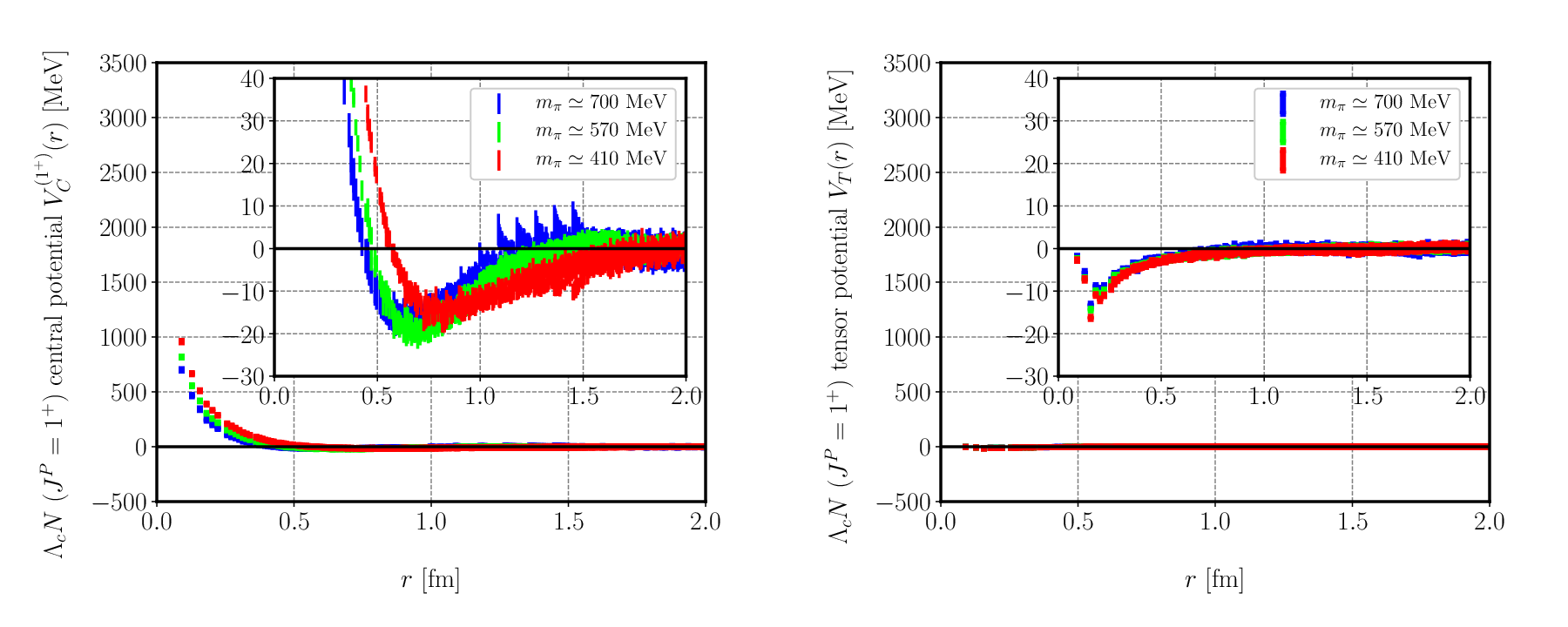
Fig. 4 shows that the central potential (left) and the tensor potential (right) for the system with . These potentials are calculated at (Ensemble 1: 700 MeV), (Ensemble 2: 570 MeV) and (Ensemble 3: 410 MeV). It is confirmed that these potentials are stable against the change of within the statistical errors, as was observed in the central potential in the channel. We notice that the central potential is similar to the one in the channel except at short distances ( fm). The tensor potential of the system is weak compared to that of the system [39]. We also find that the , quark mass dependence of the tensor potentials is weak.
The weaker potential than could be explained from following facts: (i) The long-range contribution is expected to be caused by the meson exchange for interaction [6]. In the system, however, the meson (strange quark) exchange is replaced by the meson (charm quark) exchange, and this contribution is highly suppressed due to the much heavier meson mass than the meson mass. (ii) The one-pion exchange in the transition is considered to give a sizable contribution to the effective interaction. In the system, however, this contribution is expected to be suppressed due to the large mass difference between and .
By the same procedure as in the case of the , we calculate the phase shifts and the scattering lengths in this system. Since the tensor potential is shown to be weak, we employ the effective central potential in the channel (instead of the - coupled channel), which implicitly includes the effect of the tensor potential through virtual processes such as .


4.3 Spin independence of central potentials

In this subsection, we quantify a similarity between the central potential and the effective central potential. For this purpose, we further decompose the central potential in both state (Eq. 18) and state (Eq. 24) into the spin-independent central potential and the spin-dependent one , which are extracted as
| (25) | |||
| (26) |
Fig. 7 shows the spin-independent central potential (left) and the spin-dependent one (right). It is easy to see that the spin-dependent potential is negligibly small, and the spin-independent central potential gives a significant contribution for potentials. The origin of the small spin-dependent potential could be explained by the heavy D-meson mass and the large separation between and , similar to the case of tensor potential in - channel.
5 Possible hypernuclei
Since the interaction is dominated by the spin-independent central force, as we discussed in the previous section, the spectrum of hypernuclei, if they exist, would be simple. In order to investigate hypernuclei, we employ the single-folding potential defined by
| (27) |
where denotes nuclear density distributions with the atomic number , and stands for the two body spin-independent central potential of the system.
For the nuclear density distribution function, we use the two-parameter Fermi form given by
| (28) |
where . We employ the parameters , , given in Ref. [42] for spherical nuclei such as 12C, 28Si, 40Ca, 58Ni, 90Zr and 208Pb.

Fig. 8 shows the folding potential for Pb for each ensemble. We observe that the folding potential becomes deeper as the , quark masses decrease and becomes as large as to MeV at the origin.
Using this folding potential, we calculate the binding energy of the hypernuclei by the Gaussian expansion method [43] for the -wave potential, with the physical masses for and nuclei.

Fig. 9 shows the binding energy of several hypernuclei for each ensemble. As we expected, the binding energy increases as the atomic number increases. Furthermore, as the potential approaches to the physical one (as the , quark masses decrease toward physical values), the binding energy increases. These results suggest that hypernuclei may exist, if their binding energy is larger than the Coulomb repulsion. In order to estimate the effect of Coulomb force, we calculate the expectation value for the Coulomb potential using the binding solutions of hypernulei as
| (29) |
where is the single-folding Coulomb potential defined by
| (30) |
where is an ordinary Coulomb potential and is charge density distribution by the Fourier-Bessel coefficient obtained from elastic electron scattering [44].

Fig. 10 shows the expectation values of the folding potential for Coulomb force calculated by using the binding solution of hypernuclei for Ensemble 3 ( 410 MeV). For comparison, we also plot the binding energy for hypernuclei without Coulomb potential and the sum of them in Fig. 10. We observe that the Coulomb repulsion is large for heavy nuclei and Pb state becomes unbound with Coulomb force. In the nuclei for , on the other hand, the expectation values of Coulomb force are not much stronger than the binding energy of hypernuclei. Since the binding energy increases as the attraction of the potential becomes stronger toward the physical quark mass, this observation suggests a possibility that hypernuclei may exist in light or medium-heavy nuclei.
6 Summary and conclusions
We have investigated the interaction on the basis of lattice QCD simulations. The potentials have been extracted by the HAL QCD method using the (2+1)-flavor full QCD configurations with the lattice volume of and the pion mass, MeV. We have extracted the central potential in channel and the central and tensor potential in channel. We found a repulsion at short distances and an attraction at intermediate distances in the central potentials for both channels. The strength of the attraction is weaker than that in the potential, which is consistent with phenomenological model calculations [3, 6]. For the tensor potential, we found that the strength is weaker compared with that for the system.
We next calculated phase shifts and scattering lengths using the potential fitted to the lattice data. The results show that the interaction is attractive at low energies ( MeV) in both and channels with comparable strength. In order to quantify the similarity of potentials between two channels, we decomposed the central potentials into the spin-independent and spin-dependent ones. We found that the spin-dependent potential is negligibly weak except at short distances.
The dominant contribution of the interaction comes from the spin-independent central potential, from which we have constructed a single-folding potential for hypernuclei. We then estimated the binding energies of with the nuclei, 12C, 28Ni, 40Ca, 58Ni, 90Zr and 208Pb, by using the Gaussian expansion method. Resultant binding energies of hypernuclei become larger as the atomic number increases and/or the , quark mass decreases. In order to estimate the effect of the Coulomb repulsion in the hypernuclei, we calculated expectation values of the folding potential of Coulomb force using the binding solution of hypernuclei. The expectation value of the Coulomb potential is larger than the binding energy of hypernuclei for heavy nuclei, while that is comparable to the binding energies from QCD for the nuclei with . These suggest possible hypernuclei with light or medium-heavy nuclei in the real world.
Currently, we plan to carry out full QCD simulations near the physical quark masses by using gauge configurations generated by K-computer in AICS, RIKEN. This may make it possible to draw definite conclusions on the interactions and hypernuclei. We also plan to investigate the inelastic contributions for interactions on the basis of the coupled-channel HAL QCD method [19, 23]. It is also an interesting future problem to study interactions in other two-body systems such as and , in order to understand the nature of charmed baryon interactions.
Acknowledgments
The author thanks all the members of the HAL QCD Collaboration for discussion. The author is also grateful to Shigehiro Yasui and Yasuhiro Yamaguchi for fruitful discussions and comments. This work is supported in part by the Grant-in-Aid of the Japanese Ministry of Education, Sciences and Technology, Sports and Culture (MEXT) for Scientific Research (No. JP15K17667, JP16H03978, JP17K14287, (C)26400281), by a priority issue (Elucidation of the fundamental laws and evolution of the universe) to be tackled by using Post “K" Computer, and by Joint Institute for Computational Fundamental Science (JICFuS). T.D. and T.H. are partially supported by RIKEN iTHES Project and iTHEMS Program. S.G is supported by the Special Postdoctoral Researchers Program of RIKEN. We thank the PACS-CS Collaboration for providing us their flavor gauge configurations [32]. Numerical computations of this work have been carried out by the KEK supercomputer system (BG/Q), [Project number : 14/15-21, 15/16-12].
References
- [1] R. Machleidt and I. Slaus, J. Phys. G 27 (2001) R69
- [2] E. Hiyama, T. Motoba, T. A. Rijken and Y. Yamamoto, Prog. Theor. Phys. Suppl. 185 (2010) 1.
- [3] C. B. Dover and S. H. Kahana, Phys. Rev. Lett. 39 (1977) 1506.
- [4] C. B. Dover et al. Phys. Rev. D16 (1977) 799-815.
- [5] H. Bando and M. Bando, Phys. Lett. B109, 164 (1982).
- [6] H. Bando and S. Nagata, Prog. Theor. Phys. 69, 557 (1983).
- [7] H. Bando, Prog. Theor. Phys. Suppl. 81, 197 (1985).
- [8] Y. R. Liu, M. Oka, Phys. Rev. D85 (2012) 014015, [arXiv:1103.4624 [hep-ph]].
- [9] H. Huang, J. Ping, and F. Wang, Phys. Rev. C87, 034002 (2013).
- [10] Gal, A. et al. Phys. Rev. D90 (2014) no.1, 014019, [arXiv:1405.5094 [nucl-th]].
- [11] S. Maeda, M. Oka, A. Yokota, E. Hiyama and Y. R. Liu, PTEP 2016 (2016) no.2, 023D02.
- [12] H. Garcilazo, A. Valcarce and T. F. Caramés, Phys. Rev. C92 (2015) no.2, 024006.
- [13] K. Tsushima and F. C. Khanna, Phys. Rev. C67 (2003) 015211.
- [14] K. Tsushima and F. C. Khanna, J. Phys. G: Nucl. Part. Phys. 30 (2004) 1765-1786.
- [15] N. Ishii, S. Aoki and T. Hatsuda, Phys. Rev. Lett. 99 (2007) 022001 [nucl-th/0611096].
- [16] S. Aoki, T. Hatsuda and N. Ishii, Prog. Theor. Phys. 23 (2010) 89 [arXiv:0909.5585 [hep-lat]].
- [17] S. Aoki et al. [HAL QCD Collaboration], Prog. Theor. Exp. Phys. 2012 (2012) 01A105 [arXiv:1206.5088 [hep-lat]].
- [18] T. Inoue et al. [HAL QCD Collaboration], Phys. Rev. Lett. 106 (2011) 162002 [arXiv:1012.5928 [hep-lat]].
- [19] S. Aoki et al. [HAL QCD Collaboration], Proc. Jpn. Acad., Ser. B, 87 (2011) 509 [arXiv:1106.2281 [hep-lat]].
- [20] T. Doi et al. [HAL QCD Collaboration], Prog. Theor. Phys. 127 (2012) 723.
- [21] K. Murano et al. [HAL QCD Collaboration], Phys. Lett. B735 (2014) 19 [arXiv:1305.2293 [hep-lat]].
- [22] Y. Ikeda et al. [HAL QCD Collaboration], Phys. Lett. B729 (2014) [arXiv:1311.6214 [hep-lat]].
- [23] K. Sasaki et al. Prog. Theor. Exp. Phys. (2015) 113B01 [arXiv:1504.01717 [hep-lat]].
- [24] T. Inoue et al. [HAL QCD Collaboration], PoS CD15 (2016) 020 [arXiv:1511.04871 [hep-lat]].
- [25] Okubo S., Marshak R. E., Ann. Phys. 4, 166 (1958).
- [26] K. Murano et al. [HAL QCD Collaboration], Prog. Theor. Phys. 125, 1225 (2011), [arXiv:1012.3814v1 [hep-lat]].
- [27] T. Iritani et al. [HAL QCD Collaboration], JHEP 1610, 101 (2016) [arXiv:1607.06371 [hep-lat]].
- [28] S. Aoki [HAL QCD Collaboration], PoS LATTICE 2016, 109 (2016) [arXiv:1610.09763 [hep-lat]].
- [29] T. Iritani [HAL QCD Collaboration], PoS LATTICE 2016, 107 (2016) [arXiv:1610.09779 [hep-lat]].
- [30] T. Iritani et al. [HAL QCD Collaboration], Phys. Rev. D96 (2017) no.3, 034521 [arXiv:1703.07210 [hep-lat]].
- [31] N. Ishii et al. [HAL QCD Collaboration], Phys. Lett. B712 (2012) 437 [arXiv:1203.3642 [hep-lat]].
- [32] PACS-CS Collaboration: S. Aoki, et al., Phys. Rev. D79 (2009) 034503.
- [33] S. Aoki, Y. Kuramashi and S. Tominaga, Prog. Theor. Phys. 109 (2003) 383. [arXiv:hep-lat/0107009].
- [34] Y. Namekawa, et al. (PACS-CS Collaboration), Phys. Rev. D87, 094512 [arXiv:1301.4743 [hep-lat]].
- [35] Mattia Bruno, Jacob Finkenrath, Francesco Knechtli, Björn Leder, and Rainer Sommer (ALPHA collaboration), Phys. Rev. Lett. 114 (2015) 102001 [arXiv:1410.8374 [hep-lat]].
- [36] Francesco Knechtli, Andreas Athenodorou, Mattia Bruno, Jacob Finkenrath, Björn Leder, Marina Marinkovic, Rainer Sommer, PoS LATTICE 2014 (2014) 288 [arXiv:1411.1239 [hep-lat]].
- [37] T. Doi and M. G. Endres, Comput. Phys. Commun. 184, 117 (2013) [arXiv:1205.0585 [hep-lat]].
- [38] M. Oka, K. Shimizu, and K. Yazaki, Nucl. Phys. A464 (1987) 700.
- [39] H. Nemura et al. [HAL QCD Collaboration], PoS LATTICE 2011 (2011) 167 [arXiv:1203.3320 [hep-lat]].
- [40] T. Miyamoto et al. [HAL QCD Collaboration], PoS LATTICE 2015 (2016) 090 [arXiv:1602.07797 [hep-lat]].
- [41] T. Miyamoto et al. [HAL QCD Collaboration], PoS LATTICE 2016 (2017) 117.
- [42] M. El-Azab Farid and M.A. Hassanain, Nucl. Phys. A678 (2000) 39.
- [43] E. Hiyama, Y. Kino and M. Kamimura, Prog. Part. Nucl. Phys. 51 (2003) 223.
- [44] H. De Vries, C. W. De Jager, and C. De Vries, Atomic Data and Nuclear Data Tables. 36 (1987) 495-536