Darboux Transformation for the Nonisospectral and Variable-coefficient KdV Equation
Abstract
With the nonuniform media taken into account, the nonisospectral and variable-coefficient Korteweg-de Vries equation, which describes various physical situations such as fluid dynamics and plasma, is under investigation in this paper. With appropriate selection of wave functions, the Darboux transformation is constructed, by which the multi-soliton solutions are derived and graphs are presented. The spectral parameters, coefficients and initial phase are discussed analytically and numerically to demonstrate their respective effect on the soliton dynamics, which plays a role in achieving the feasible soliton management with explicit conditions taken into account.
PACS numbers: 05.45.Yv, 02.30.Ik, 47.35.Fg
Keywords: Nonisospectral Korteweg-de Vries equation; Darboux transformation; Soliton management; Integrability
I. Introduction
The Korteweg-de Vries-type (KdV-type) equations are of current interest in describing the physical situations such as wave motion, ion-acoustic wave, Bose-Einstein condensates and arterial dynamics [2, 7, 3, 1, 5, 4, 6, 8]. By appropriate model construction, KdV-type equations with certain coefficients have been investigated analytically by inverse scattering method [10, 9], direct method [11, 12], Wronskian technique [14, 13], Darboux transformation [15, 16, 17, 19, 18] and so on [20, 21, 22], among which, the Darboux transformation (DT) is a purely algebraic iterative tool to generate soliton solutions [15, 16, 17, 19, 18].
It is shown that an integrable system may possess more than one DT [15] and so far various forms of DT have been investigated for different kinds of KdV-type equations. For instance, a more general DT is constructed for the Hirota-Satsuma-KdV equation, which is quadratic in the spectral parameter [16], the DT with an arbitrary parameter is utilized for the study of integrable sixth-order KdV equation [17], a vectorial DT with ordinary determinants is applied for the supersymmetric extension of KdV equation [18], and the generalized binary DT is used to obtain the negaton, positon, and complexiton solutions of nonisospectral KdV equations with self-consistent sources [19].
With the nonuniform media taken into account, the KdV-type equations are related to time-dependent spectral parameters with relaxation [25, 26, 28, 24, 29, 23, 27]:
| (1) |
under appropriate coefficient selections which may model for the problem of tunnelling of solitons across density humps [23] and indicate the reflectionless potentials for nonisospectral KdV hierarchy [24]. With a certain balancing between the loss and the nonuniformity in media [25], the nonisospectral characteristics of the motion behaviours of some solutions are described [26] and the symmetry structure is studied [27]. Taking self-consistent sources in nonlinear media into account, Eq. 1 can be extended and investigated [29, 28].
By virtue of the constraint below [30], which reduce the degrees of restriction among various coefficients, Eq. (1) is an integrable system,
| (2) |
where is a non-zero constant.
However, to the best of our knowledge, the DT for Eq. (1) has not been constructed under the general constraint (2). Hereby in this paper, we will construct a DT of Eq. (1) and provide analytical and numerical discussion about the solitonic dynamic under the effect of spectral parameters, coefficients and initial phases respectively.
In Section II, the DT for Eq. (1) under constraint (2) is constructed. In Section III, the soliton solutions are derived in explicit forms, with the soliton-like solutions being generated and presented graphically. In Section IV, we investigate the effects of spectral parameters, coefficients and initial phases on the solitonic dynamic, as well as present the graphic illustration of the soliton propagation and interactions. In Section V, numerical simulation is applied to further discuss the soliton activities with the constraint (2) perturbed. Finally, the conclusions are offered in Section VI.
II. Construction of DT
In this section, we will construct a DT of Eq. (1) under the Lax pairs [30]
| (3) |
| (4) |
where is defined as wave function with and being a real constant. The spectral parameter satisfies the conditions of Lax pair by .
The DT can be constructed with undetermined time-varying coefficients A(t), B(t) and C(t) as below,
| (5) |
and
| (6) |
in which subscript represents iteration of DT and the satisfying Lax pairs is a real function of and . The particular solution is defined as .
Define the as an induction function for its role in the transformation process. Notice that and are the original solutions of the Lax pairs and Eq. (1), respectively, with and derived from as new solutions by a DT.
Spectral parameter is a time-varying function, which should comply with the conditions of the Lax pair and is given by
| (7) |
where is a real constant, reflecting the size of value in the spectral parameter when is given. In the discussion later, we study the spectral parameter by discussing the value of .
Applying the undetermined expressions (5) and (6) into the following compatibility condition of Lax pair (3) and (4)
| (8) |
and finish it by comparative coefficients method, we obtain the specific coefficients of DT (5) and (6)
| (9) |
| (10) |
| (11) |
Therefore, we can construct the explicit form of DT as following,
| (12) |
and
| (13) |
in which = and is derived from by an iteration of DT. Notice that each step of DT utilizes a specified parameter for derivation of new solution.
II. Generations by DT
In this section, we will discuss the generated solutions for Eq. (1) under different forms of wave functions by DT.
Employ as the original solution for Eq. (1) and suppose that the original solution of wave function has the following form
| (14) |
where and are functions of to be determined.
Substituting above equation into Lax pair (3) and (4), we have
| (15) |
and
| (16) |
in which is an arbitrary constant, representing the soliton initial phase.
By means of expression (14), an induction solution is constructed by = with a given value . Hereby, we obtain a single-soliton solution by a DT (12).
We have
| (17) |
where
| (18) |
| (19) |
in which is the initial phase with the subscript representing the first iteration of DT.
To derive wave function , we employ a different wave function defined as
| (20) |
where and are as same as the expression (15) and (16) respectively. Therefore, we can obtain another wave function by a DT (13) using and , which paves the way for deriving two-soliton solution.
| (21) |
To obtain two-soliton solution, we utilize a second DT (12) with an induction solution corresponding to the wave function (21),
| (22) |
where . The derived two-soliton comply with the basic law of nature in its propagation and interaction dynamic. An example is presented below in Fig.1 (a).
By the induction solution corresponding to Eq. (14) without adjustment, the solutions for Eq. (1) can also be generated, but with considerable singularity in rational field. As shown in Fig.1 (b), the soliton-like graphs are presented.


() ()
The difference between the generated solutions derived by the original wave function (14) and the adjusted wave function (20) indicates the necessary modification when constructing DT in the form of operator in order to derive soliton solutions. As shown in Fig.2 (a) and (b), the solution iterated by DT can be further extended to multi-soliton solution.


() ()
IV. Discussions
Generally speaking, the interaction and propagation of soliton dynamics play a role in determining the physical feature and benefit the applicants of dynamical system. Therefore, in this section, we will investigate the respective influence of spectral parameters, different coefficients and initial phases on the solitonic velocity, width, amplitude, demonstrating the figure of solitonic dynamic in fluid.
Case A. Eq. (1) is related to the time-dependent spectral parameter , which could describe the solitons wave in nonhomogeneous media [2, 7].
() ()


() ()
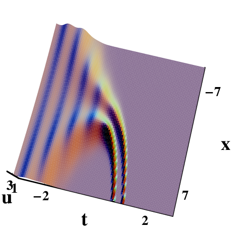
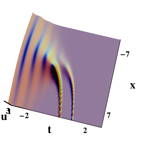
As shown in Figs.3 (a) and (b), when spectral parameter increases, the interaction of solitons become intensifier, with the amplitude aggraded and the wide narrowed. Consider Figs.3 (a), (c) and (b), (d), respectively, with time passing by, the solitons propagate longer distance at the same time interval. In each graph, the soliton with higher amplitude generates a faster speed compared with the other one. Compare Figs.3 (a), (c) with (b), (d), as spectral parameter increases, the elevation soliton experiences a growth of velocity and amplitude. It is shown in Fig.3 (b) that when there is an noticeable imbalance between spectral parameters, a soliton dynamic feature is almost covered by the other at the intersection.
It is worth noting that when , the two-soliton solution is degenerated to constant value zero.
By an appropriate selection of the , we can construct negative spectral coefficients in the following graph. The phenomena in the Fig.4 can be also interpreted by the influence of spectral parameters. When is balanced with , the solitons converge into one at the intersection.


() ()
Case B.
From the expression (17), the solitonic amplitude can be interpreted as , where the is the only time-dependent coefficient.


() ()
By a positive application of line-damping coefficient , the soliton management for time-space locality is achieved. As demonstrated in Fig.5 (b) by the profile at certain time, the solitonic amplitude get enhanced when time is approaching to zero and then attenuated as time keeps going on, besides, the space influenced by solitonic dynamics is limited locally. The depression of solitons amplitude can be interpreted by the term analytically.
Case C.
The coefficient indicates the inhomogeneities of media, which affects the solitonic dynamical behavior.


() ()
As shown in Figs.6 (a) and (b), by choosing the negative and positive value corresponding to the nonuniformity coefficient , the solitons swell and shrink over time, respectively. It is worth noting that the degree of solitonic broadening and compressing depends on the absolute value of . The influence of variable coefficients on the soliton dynamics is similar to that in Refs [31, 30].
Case D. In case D, based on expression (22), the effect of the initial phases will be discussed and presented graphically.


() () ()
The initial phase and result from the first and second step of DT, respectively. As shown in Fig.7 (a), the solitons interact with each other and generate a phase shift at the intersection. By an increment of initial phase , Figs.7 (a), (b) and (c) demonstrate a position displacement of the related soliton, with the other soliton dynamics almost unchanged. By a proper use of initial phase, we may obtain individual solitonic management and induce an interaction. With periodical time-dependent in Fig.7, the solitonic physical feature also corresponds to the interpretation of line-damping coefficient above, which demonstrates that the periodical amplitude fluctuation of solitons is generated by the time-periodical value of coefficient .


() ()
It is worth noting that a sign change of the initial phase distance will lead to an exchange of solitonic position, with the height nearly unchanged, which is shown in Fig.8. When the initial phase is appropriately modified, we can generate a solitonic position exchange in space.
V. Numerical Simulation
For solitonic generation, the constraint is necessary to balance the nonlinearity and dispersion, under which our analytical solitons-solution is constructed. In this section, when the constraint (2) is perturbed, the numerical simulation is applied to further discuss the influences of coefficients on the solitonic velocity, amplitude and width.
Employ one-soliton solution (17) with coefficients and parameters , we have
| (23) |
Take as the initial analytical solution and by finite difference method, we have the numerical solution .
By perturbation on the coefficients , and , respectively, we have the numerical simulations presented below.


() ()


() ()
From the view of Fig.9, the consistence between the numerical and analytical solitonic profiles at is well demonstrated when constraint (2) is satisfied.
As shown in Fig.9, the positive (negative) perturbation on dispersive coefficients will lead to slight numerical shock as space expands, with decrease (increase) on velocity and amplitude. By numerical simulation, coefficient has an inhibitory effect on the amplitude of solitons, which is similar to the analytical discussion under constraint in Section IV. The decrease on demonstrates slow-down effect on solitons velocity with the amplitude almost unchanged. The negative perturbation on results in the decrease of soliton width, while the positive perturbation can lead to the widening.
IV. Conclusions
In this paper, with the nonhomogeneous media taken into account, we have investigated the nonisospectral and various-coefficients KdV equation (1). Under the general constraint (2), the DT (12) and (13) is constructed with the adjustments applied to generate the solitons solutions. By virtue of DT, the multi-soliton solutions are iterated from the seed solution.
The soliton dynamics might describe different physical phenomena and benefit the relevant applications in various fields. Therefore, by virtue of analytical discussion, we discuss the effect of spectral parameters, coefficients, and initial phases on the solitons dynamics. The conclusions inferred from the above discussions can be presented as follow:
(1) As demonstrated in Fig.3, the increase (decrease) of spectral parameter might induce the growth (fall) of the solitons amplitude and velocity. With appropriate selection of spectral parameters and , the multi solitons might converge into one at the intersection.
(2) As shown in Fig.5 and Fig.6, with the proper selection of line-damping coefficient , we can obtain the space-time locality of solitons. Besides, the solitons compression (widening) depends on the sign of coefficient .
(3) As illustrated in Fig.7 and Fig.8, by modulating the initial phases, we can generate the solitons interaction and position exchange.
Moreover, with the constraint taken into account, the numerical simulation result in Fig.9 is consistent with the analytical discussion. With the constraint (2) perturbed, the effect of respective coefficient is also studied.
It is demonstrated that the amplitude, width and velocity of solitons could be modulated by appropriate selection and combination of the coefficients and parameters. Therefore we can achieve the purpose of soliton management with explicit conditions taken into account.
Acknowledgements
We express our sincere thanks to Editor, Referees and all the members of our discussion group for their valuable comments. This work has been supported by the National Natural Science Foundation of China under Grant No. 11302014, and by the Fundamental Research Funds for the Central Universities under Grant Nos. 50100002013105026 and 50100002015105032 (Beijing University of Aeronautics and Astronautics).
References
- [1] Z. Y. Yan, Appl. Math. Com. 217, 9742, 2011.
- [2] H. Demiray, Chaos. Soliton. Fract. 42, 1388, 2009.
- [3] B. Tian, G. M. Wei, C. Y. Zhang, W. R. Shan and Y. T. Gao, Phy. Lett. A 356, 8, 2006.
- [4] G. Gottwald, R. Grimshaw and B. Malomed, Phys. Lett. A 227, 47, 1997.
- [5] J. K. Xue, Phys. Lett. A 322, 225, 2004.
- [6] S. C. Li, J. N. Han and W. S. Duan Phys. B 404, 1235, 2009.
- [7] H. Demiray, Int. Jour. Nonl. Mech. A 43, 241, 2008.
- [8] W. S. Duan, Y. R. Shi, X. R. Hong, K. P. L and J. B. Zhao, Phy. Lett. A 295, 133, 2002.
- [9] W. L. Chan and K. S. Li, J. Math. Phys. 30, 2521, 1989.
- [10] W. L. Chan and X. Zhao, J. Phys. A 28, 407, 1995.
- [11] X. G. Xu, X. H. Meng, F. W. Sun and Y. T. Gao, Mod. Phys. Lett. B 24, 1023, 2010.
- [12] L. L. Li, B. Tian, C. Y. Zhang, H. Q. Zhang, J. Li and T. Xu, Int. J. Mod. Phys. B 23, 2383, 2009.
- [13] X. G. Xu, X. H. Meng and Y. T. Gao, Chin. Phys. Lett. 25, 3890, 2008.
- [14] S. F. Deng, Commun. Theor. Phys. 43, 961, 2005.
- [15] H. C. Hu and Q. P. Liu, Chaos. Soliton. Fract. 17, 921, 2013.
- [16] L. L. Xue, Q. P. Liu and D. S. Wang, Jour. Math. Phys. 57, 083506, 2016.
- [17] X. Y. Wen, Y. T. Gao and L. Wang Appl. Math. Com. 218, 55, 2011.
- [18] Q. P. Liu and M. Manas, Phys. Lett. B 394, 337, 1997.
- [19] J. S, W. Xu, G. J. Xu and L. Gao, Commun. Nonlinear. Sci. Numer. Simulat. 17, 110, 2012.
- [20] X. Q. Zhao, D. B. Tang and L. M. Wang, Phys. Lett. A 346, 288, 2005.
- [21] W. L. Chan and K. Y. Zheng, Lett. Math. Phys. 14, 293, 1987.
- [22] S. S. Ding, W. J. Sun and D. C. Zhu, Appl. Math. Comput. 199, 268, 2008.
- [23] M. R. Gupta, Phys. Lett. 72A, 6, 1979.
- [24] T. K. Ning, D. Y. Chen and D. J. Zhang, Chaos. Soliton. Fract. 21, 395, 2004.
- [25] R. Hirota and J. Satsuma, J. Phys. Soc. Jpn. (Lett.) 41, 2141, 1976.
- [26] D. J. Zhang and D. Y. Chen, J. Phys. A 37, 851, 2004.
- [27] J. F. Zhang and P. Han, Chin. Phys. Lett. 11, 721, 1994.
- [28] H. H. Hao, G. S. Wang and D. J. Zhang, Commun. Theor. Phys. 51, 989, 2009.
- [29] Q. Li, D. J. Zhang and D. Y. Chen, J. Phys. A. Math. Theor. 41, 355209, 2008.
- [30] X. Yu, Y. T. Gao, Z. Y. Sun and Y. Liu, http://www.paper.edu.cn/index.php/default/ releasepaper/content/201204-236 , 2012
- [31] X. Yu, Y. T. Gao, Z. Y. Sun and Y. Liu, Phys. Rev. E 83, 056601, 2011; X. Yu, Y. T. Gao, Z. Y. Sun and Y. Liu, Phys. Scr. 81, 045402, 2010.