Differentially Private Query Learning: from Data Publishing to Model Publishing
Abstract
With the development of Big Data and cloud data sharing, privacy preserving data publishing becomes one of the most important topics in the past decade. As one of the most influential privacy definitions, differential privacy provides a rigorous and provable privacy guarantee for data publishing. Differentially private interactive publishing achieves good performance in many applications; however, the curator has to release a large number of queries in a batch or a synthetic dataset in the Big Data era. To provide accurate non-interactive publishing results in the constraint of differential privacy, two challenges need to be tackled: one is how to decrease the correlation between large sets of queries, while the other is how to predict on fresh queries. Neither is easy to solve by the traditional differential privacy mechanism. This paper transfers the data publishing problem to a machine learning problem, in which queries are considered as training samples and a prediction model will be released rather than query results or synthetic datasets. When the model is published, it can be used to answer current submitted queries and predict results for fresh queries from the public. Compared with the traditional method, the proposed prediction model enhances the accuracy of query results for non-interactive publishing. Experimental results show that the proposed solution outperforms traditional differential privacy in terms of Mean Absolute Value on a large group of queries. This also suggests the learning model can successfully retain the utility of published queries while preserving privacy.
I Introduction
With advances in Big Data and online services, Privacy Preserving Data Publishing (PPDP) has attracted substantial attention [17]. In the past few years, a number of privacy definitions and mechanisms have been proposed in the literature. Among them, the most influential one is the notion of differential privacy [5], which constitutes a rigorous and provable privacy definition. Existing work on differential privacy has mainly focused on interactive publishing, in which the curator releases query answers one by one [4]. However, curators have to releases a large number of queries or a synthetic dataset in may Big Data scenarios such as machine learning or data mining [4]. The existing differentially private method fails to provide accurate results when publishing a large number of queries. [12]. This obstacle hinders the implementation of differential privacy in Big Data applications.
The difficulty in non-interactive data publishing lies on the high correlation between multiple queries [9]. High correlation leads to large volume of noise adding to the query results. Given a fixed privacy level, noise is determined by the sensitivity. The sensitivity is defined to capture the difference in the query results between the addition or removal of a single record in a dataset. When answering a query set, a curator has to calibrate the sensitivity of these queries, but as deleting one record may affect multiple query answers. In another word, the queries in the set may correlate to one another. Correlations between queries lead to higher sensitivity (normally multiplied by the original sensitivity) than independent queries [9]. The problem is illustrated in the following example.
I-A An Example
Table I shows a frequency dataset with variables, and Table II contains all possible range queries . As changing any value in will impact on at most query results (column containing or in Table II) in , the sensitivity of is , which is much higher than the sensitivity of a single query. The noise will be added to every query in . The sensitivity of is and the variance of the noise per answer is . When is large, the utility of the results will be demolished. Alternatively, Laplace noise can be added to and the range query results are generated accordingly. In this situation, the sensitivity is , but the privacy budget has to be divided into pieces and arranged to each query in , leading even higher noise than the previous method.
This example shows that traditional publishing methods introduce a large volume of noise and lead to inaccurate results, while how to reduce noise remains a major problem in non-interactive publishing.
I-B Challenges and Rationale
| Grade | Count | Variable |
|---|---|---|
| Range Query | |||||||
|---|---|---|---|---|---|---|---|
| + | + | + | |||||
| + | + | ||||||
| + | + | + | |||||
| + | |||||||
| + | + | ||||||
| + | |||||||
The above example illustrates that two challenges need to be tackled in the non-interactive publishing.
- •
How to decrease correlation among queries? As the correlation among queries will introduce large noise, and this high volume of noise must be added to every query according to the definition of differential privacy. We have to decrease the correlation to reduce the introduced noise.
- •
How to deal with unknown fresh queries? As the curator cannot know what users will ask after the data has been published, he/she has to consider all possible queries and adds pre-defined noise. When we meet with the scenarios in Big Data, it is impossible to list all queries. Even if the curator is able to list all queries, this pre-defined noise will dramatically decrease the utility of the publishing results.
Several works have been carried out over the last decade to address the first challenge by a strategy. Let’s use the above example again. If we only need to answer to , the sensitivity of the query set is decreased to and other query results can be generated by the combination of to . For example, the answer of can be generated by and . The solution looks quite simple and effective and most existing work are following this strategy to decrease the correlation. Xiao et al. [14] proposed a wavelet transformation to decrease the correlation between queries. Li et al. [12] applied the Matrix method to transform the set of queries into a suitable workload. Similarly, Huang et al. [9] transformed the query sets into a set of orthogonal queries. However, they can only partly solve the first challenge, while the second challenge has not been touched by these methods. For complex queries, such as similarity queries, it is hard for a curator to figure out all independent queries. In addition, when given a fresh new query, how did the curator generate the result by combining of old queries is still remain unknown.
We observe that these two challenges can be overcome by transferring the data publishing problem to a machine learning problem. We treat the queries as training samples which are used to generate a prediction model, rather than releasing a set of queries or a synthetic dataset. For the first challenge, correlation between queries, we will apply limited queries to train the model. These limited queries have lower correlation than in the original query set. If we can guarantee the training queries can cover most possible scenarios, the output model will have higher prediction capability.
For the second challenge, the model can be used to predict the remaining queries, including those fresh queries. Actually, the model prediction is to generate the combination of training queries. Consequently, the quality of the model is determined by two key factors: the coverage of the training samples and the prediction capability of the prediction model. The model can help to answer unlimited number of complex queries.
In the above example, if we use to as the training samples, the sensitivity will be diminished to and the added noise will be decreased accordingly. The prediction model can be used to answer to . Because the prediction process will not access original dataset , it will not consume any privacy budget.
The target of this paper is to propose a novel differentially private publishing method that can answer all possible queries with acceptable utility. We make the following contributions:
- •
We propose a novel differentially private data publishing method, MLDP, which successfully transfers the data publishing problem to a machine learning problem, solving the current challenges of non-interactive data publishing. This method exploits a means of publishing more types of data, such as a data model.
- •
We analyze both the privacy and the utility of MLDP, demonstrating that the MLDP satisfies -differential privacy and proving the accuracy bound of the MLDP.
- •
We use extensive experiments on both real and a simulated dataset to prove the effectiveness of the proposed MLDP. After comparing our method with traditional Laplace and other prevalent publishing methods, we conclude that the MLDP demonstrates better performance when answering a large set of queries.
II Preliminaries
II-A Notation
We consider a finite data universe with the size . Let be a record with attributes sampled from the universe , while a dataset is an unordered set of records from domain . Two datasets and are neighboring datasets if they differ in only one record. A query is a function that maps dataset to an abstract range : . A group of queries is denoted as , and denotes . We use symbol to denote the number of queries in .
The maximal difference on the results of query is defined as the sensitivity , which determines how much perturbation is required for the private-preserving answer. To achieve the target, differential privacy provides a mechanism , which is a randomized algorithm that accesses the database. The randomized output is denoted by a circumflex over the notation. For example, denotes the randomized answer of querying on .
II-B Differential Privacy
The target of differential privacy is to mask the difference in the answer of query between the neighboring datasets [5]. In -differential privacy, parameter is defined as the privacy budget [5], which controls the privacy guarantee level of mechanism . A smaller represents a stronger privacy. The formal definition of differential privacy is presented as follows:
Definition 1 (-Differential Privacy)
A randomized algorithm gives -differential privacy for any pair of neighboring datasets and , and for every set of outcomes , satisfies:
| (1) |
Sensitivity is a parameter determining how much perturbation is required in the mechanism with a given privacy level.
Definition 2 (Sensitivity)
[5] For a query , the sensitivity of is defined as
| (2) |
The Laplace mechanism adds Laplace noise to the true answer. We use to represent the noise sampled from the Laplace distribution with the scaling . The mechanism is defined as follows:
III The Machine Learning Differentially Private Publishing method
III-A Overview

This section presents the implementation of the Machine Learning Differentially Private (MLDP) publishing method. For an original dataset , suppose a set of query on the is waiting to be published. Fig. 1 presents the flow of the traditional Laplace method and the MLDP method. The first flow shows the method. When the is querying on , the method will measure the sensitivity of the query set . To simplify the notation, we re-write the sensitivity of a group of queries in definition 4.
Definition 4 (Sensitivity for Correlated Queries)
Given a group of queries over a dataset , Equation. 4 provides the sensitivity of .
| (4) |
Based on the definition, the sensitivity of is . The Laplace noise is calibrated by and is added to the true answer . The Laplace method finally outputs the noisy answer .
The second flow presents the MLDP method. Unlike the traditional Laplace method, it first selects a query set for training. Sensitivity is measured and noise is added to query answers. Training set is carefully selected to make sure . When a learning model is generated, it will accept the query set and make the prediction . The MLDP method eventually outputs .
Comparing with the Laplace method, the proposed MLDP adds less noise in the training set than that in the Laplace method. This is because normally has correlation with others, while can be selected with lower correlation. According to Definition 4, will be smaller than . A smaller sensitivity leads to less noise. This helps to solve the first challenge, high correlation problem in the Laplace method. In addition, prediction model accepts fresh queries, which are unknown to the curator before data publishing. Eventually, these two properties of MLDP help to tackle those two challenges in traditional Laplace method.
III-B Implementation of MLDP
At a high level, MLDP works in three steps:
- •
Generating training samples: The curator selects a query set with queries to generate training samples.
- •
Training the model: The training set is used to train a prediction model . In theory, we can select any machine learning algorithm. As most of the query answers are numerical values, regression algorithms will be more suitable.
- •
Making prediction: The model is applied to make prediction of fresh queries . The prediction results will be output as the noisy answer of those queries.
Algorithm 1 illustrates the detail of the MLDP method. At the first step, we measure the sensitivity of the training sample . Because is a subset of , will be smaller than and the noise added to will be diminished accordingly. At Step , Laplace noise is added to the true answer and we obtain the noisy answer . Step generates the training set . Step uses to learn a regression model and consider it to be a synopsis of the original dataset . At Step , model will be released to the public and every time public users try to query the dataset , the answer is predicted by the model .
III-C Training set Selection
The performance of the model is affected by two types of errors. One is noise error , which is incurred by noise added to the training set. Another is model error , which is triggered by the inaccuracy of the learning model. According to the union bound, the probability of the total error can be defined as
| (5) |
We define two criteria to measure the selection of training set. One is independent, which means how many queries are issued on one variable. The independent is highly related to the sensitivity: a high independent training set leads to lower sensitivity. Therefore, when queries in training set are independent to others, the noise error will be lower.
Another criteria is coverage, which means how many variables can be covered by the training set. It is obviously that if some variables cannot be covered by the training set, the model error will be very high. On the other hand, if one query covers all variable, the model error will still be very high as the model will be less fitting.
III-D Training the Model and Making Prediction
Model can be trained by various learning algorithms, for example, linear combinations of fixed nonlinear functions of the input variables can be used to train a model .
| (6) |
where is the Gaussian basis function, as shown in Equation 7.
| (7) |
where is the average value of and is a pre-defined parameter to control the scalability of the basis function. When model is generated, queries, including fresh queries answers can be generated by without consuming any privacy budget.
In fact, the model depicts the combination of varies queries answers. For example, the linear regression model for range queries is approximate to a histogram publishing. The parameters in a linear regression model are actually frequencies of a histogram. But the linear regression model is not working well for the similarity query, this is the because the combination of similarity queries are more complex comparing to range queries, while a more sophisticated model is needed in this case, such as the neural network, SVM models. The effectiveness of these learning algorithms will be proved in the experiment.
IV Analysis of the MLDP
IV-A Privacy Analysis of the MLDP Method
According to the definition of differential privacy, if the data processing follows the requirement of differential privacy at each step, the result will satisfy with differential privacy [5].
Algorithm 1 shows that the privacy budget is only consumed in Step , in which Laplace noise is added to answers of training queries . As the original dataset is only accessed by , following steps, model training and fresh query prediction, will not disclose any privacy information. Therefore, we ensure every step in Algorithm 1 satisfies differential privacy.
In addition, the model will be published to the public to make prediction. No matter what type of learning algorithms we choose to train the model, it contains noise that will not release any privacy information. Similar to other non-interactive data publishing methods, once is published, the privacy level of the model is fixed by that MLDP consumes in the training step. In general, we have transferred the differentially private non-interactive data publishing problem into a machine learning problem with the constraint of differential privacy.
IV-B Utility Analysis of the MLDP Method
In this section, we focus on the relationship between the size of the training set and the accuracy of the query result. The accuracy is determined by a widely used utility notion in differential privacy suggested by Blum et al. [1]:
Definition 5 ((,)-useful)
A mechanism is (,)-useful for a set of queries and a dataset , if: with probability , for every query , we have
| (8) |
then is the accuracy of the method and is the confidence parameter.
Equation 5 will help us to analyze the utility of MLDP. Based on the accuracy definition and the relationship between errors, we will demonstrate that errors of MLDP are bounded by a certain value with high probability.
The model error is associated with the type of query and the learning algorithm. As MLDP does not specify the query type, we can use the range query as an example. When a dataset has records, the range query will output true values in a range from to . For other types of queries, the difference is only in the range of query answers in the bound. MLDP also does not specify the learning algorithm. We suppose the learning algorithm we choose has a hypothesis set with size . The accuracy bound of model error will be estimated by Theorem IV.2 and will be proved with the help of the Chernoff-Hoeffding bound [10].
Lemma IV.1
(Real-valued Chernoff-Hoeffding Bound) [10]. Let be independent random variables with and for all i, then for every ,
| (9) |
Theorem IV.2
For any query , all , with probability at least , the model error is bounded by , where dependents on the learning algorithm we choose for MLDP.
Proof. As , we have
and
As range query result is a true value with the maximum value of and the minimum value of , according to Lemma IV.1, for every hypothesis , we have
For all hypotheses, we then have
Let , We have .
The noise error is independent to the query type and the learning algorithm, and can be analyzed by the property of Laplace noise, which is presented by sums of Laplace random variables in Lemma IV.3.
Lemma IV.3
(Sums of Laplace Random Variables) [10]. Let be a set of independent random variables drawn from Laplace(), then for every ,
| (10) |
In the MLDP training set, the noise is derived from . Theorem IV.4 shows the bound of the .
Theorem IV.4
For any query , all , with probability at least , the noise error of MLDP is bounded by , where dependents on the learning algorithm we choose for the MLDP.
Proof. As , we have
For each , MLDP adds a random variable as noise drawn from . When , we need to bound . According to Lemma 2, we have
For all hypotheses , we then have
Let , we have .
Theorem IV.2 illustrates the relationship between the accuracy and the size of the training set. The bound on indicates that a larger size of training set results in a lower and higher accuracy. Theorem IV.4 shows that the accuracy is also associated with the sensitivities . A larger leads to larger and lower accuracy. As is dominated by the correlations between queries in the training set, a larger will increase . Although a large increases the accuracy according to Theorem IV.2, will be enlarged at the same time which will impede the enhancing of the accuracy. These results assist in selecting the training set of the MLDP.
To retain acceptable accuracy, we cannot use all possible queries to train the model. At first glance, it seems that if we can list all possible queries as the training set, we can produce a very accurate model to make the prediction. However, according to Theorem IV.4, even though a large training set results in less model error , a large training set contains huge number of correlated queries, which leads to higher sensitivity and large noise error . The total error will be quite large and the accuracy will be reduced.
We cannot use only the uncorrelated queries as the training set. In this case, can be quite small due to the smaller sensitivity and lower volume of noise; however; as uncorrelated queries are only a small proportion of the entire number of queries, the model will be very inaccurate and will be very large. Both cases indicate that we must consider two types of error to achieve better performance.
IV-B1 Advantage of MLDP
There are several advantages to using a machine learning method to deal with the non-interactive publishing problem:
- •
Many machine learning models can be applied to the data publishing problem. For example, we can use linear regression, SVM for regression and neural network to learn a suitable model according to the training set. As prediction is a mature area that has been investigated in machine learning for several decades, we can choose sophisticated technologies and adjust parameters to obtain a better performance.
- •
Some existing methods can be considered as an extension of MLDP. For example, the Private Multiplicative Weights (PMW) Mechanism [7] is one of the most prevalent publishing methods in differential privacy. To some extent, it can be considered as an instance of the MLDP method. In the PMW, the histogram is a selected model and frequencies in this histogram constitute parameters of the model. The model (histogram) is trained by the input queries until it converges or meets the halting criteria. Compared to MLDP, however, PMW can only answer queries in the training set.
- •
The noisy model naturally has the property of generalization. Generalization is an essential problem in machine learning, but the differential privacy mechanism has proven that it can avoid over-fitting in the learning process [6].
IV-C Differences between MLDP and Private Learning
The proposed MLDP method is highly related to machine learning algorithms, but is different to previous private learning. It is a method that introduces noise into the original learning algorithms, so that the privacy of the training dataset can be preserved in the learning process [10]. First, the purpose of publishing models is different. MLDP aim to publish a model for fresh query prediction, whereas private learning is only used for traditional machine learning tasks and will not preserve the privacy of fresh samples.
Second, MLDP considers pre-defined queries as a training set while private learning considers records in the original dataset as traninig samples. The target of differential privacy is to hide the true value of query answers, not the records, so MLDP considers the query as the training sample and the model is used to predict query answers rather than the values of records. In this respect, MLDP is totally different from private learning algorithms. Even though Kasiviswanathan [10] proved that Kearn’s statistical query (SQ) [11] model can be implemented in a differentially private manner, the training set still comprises records in the dataset. Consequently, the SQ model is similar to private learning, not MLDP.
Finally, as public users normally use count, average or sum query, MLDP normally applies regression algorithms for true value prediction, while the private learning algorithm is usually specific to classification with labels of or . Table III summarizes the major differences between MLDP and private learning.
| MLDP | Private Learning | |
|---|---|---|
| Model | The model is used to predict fresh query answers for public users | The model is used for traditional machine learning |
| Training set | Queries on the dataset | Records in the dataset |
| Protect Target | Preserve the privacy of all queries. | Do not protect future samples |
| Learning Algorithms | Prediction | Classification |
V Experiment and Analysis
V-A Experiment Configuration
The experiments involve four datasets. Three are derived from Hay’s work [8], and have been widely used in the differentially private publishing tests.
- •
NetTrace: this dataset contains the IP-level network trace at a border gateway of a university. Each record reports the number of external hosts connected to an internal host. There are records with the number of connections ranging from to .
- •
Search Logs: this synthetic dataset was generated by interpolating Google Trends data and America Online search logs. It contains search records collected between Jan. 1, 2004 and Aug. 9, 2009.
- •
Social Network: this dataset records the friendship relations among students, sampled from an online social network website. There were students, each of which had at most friends.
- •
Netflix The Netflix dataset is extracted from the Netflix Prize dataset, where each user rated at least movies, and each movie was rated by users. This dataset is used to test the similarity query.
- •
Simulated Histogram: this simulated histogram contains bins with random numbers. The target of the simulated histogram is to list all possible queries. For a histogram with queries, the range query number is . We will test all the queries in the experiment.
- •
Netflix: the Netflix dataset is extracted from the Netflix Prize dataset, where each user rated at least movies, and each movie was rated by users. This dataset is used to test similarity queries.
We select different learning algorithms, including linear regression, neutral network, ensemble bag, boost, and SVM, to create prediction model. Two types of queries will be tested based on the prediction model: range query and similarity query. Range query is normally presented as how many users are there in the dataset with the age from 20 to 40? Range query is actually a count related query, which count how many record that meet with a specified property. Similarity query is a type of complex query that measures the similarity between two records. For example, what is the similarity between those two users in terms of their preference on movies? For both range and similarity queries, ¿¿¿¿¿¿¿ .r2804 we generated a training set with random queries . These range queries are correlated to one another and the sensitivity is measured by definition 4. The accuracy of results was measured by Mean Absolute Error (MAE).
| (11) |
A lower MAE implies better utility.
V-B Model Selection
To select the model that fits for a particular type of query, several algorithms have been tested with , including regression, SVM, neural network, bagging, and boosting. Figure 2 shows the results on Social Network and Netflix datasets. Figure 2a illustrates that regression algorithm outperforms other algorithms in terms of the range query. When the size of the training set increases, the MAE of the regression decreases dramatically. When the size of the training set increases to more than , MAEs of all algorithm are stable. These mean that the regression algorithm can be fully trained in limited training samples, while others need more training samples.
However, for similarity queries, the performance of regression is worse than others. As shown in Figure 2b, the SVM algorithm has the lowest MAE comparing with other algorithms. This is because the similarity query needs complex combination that cannot be deduced easily. The SVM algorithm is more suitable to simulate the combination of queries. Due to limited space, we only used range query and regression model as examples in following set of experiments.


V-C Performance of MLDP with Different Sizes of Training Set


The theory analysis in Section indicates the size of the training set plays a vital role in prediction. This experiment examines various sizes of training set and test set. We set the size of training sets from to , and set two different sizes of test query, and , respectively. The result is compared with the traditional Laplace method and the is fixed at .
Fig. 3 shows the impact of the size of the training set on the performance of MLDP. Initially, it is apparent that MAE drops quickly with the increase in , but when is larger than a certain value, the MAE reaches its minimum and continues to increase. As shown in Fig. 3a, the MAE keeps decreasing until , with at its lowest point. As subsequently increases, the MAE keeps rising until , until it reaches . The MAE then goes down slowly as increases. When it reaches another inflexion, the MAE slowly rises. This result is consistent with Theorem IV.2 and IV.4 in Section IV-B, in which the performance of MLDP is impacted by the mixture of noise error and model error. The model error plays a dominate role when is small, so the MAE decreases with increasing. Beyond the threshold, however, the noise error dominates the results. As a larger introduces a larger volume of noise, so the MAE is enhanced.
Similarly, Fig. 3c shows that the MAE reaches its minimum when . Fig. 3e and Fig. 3g show the same trend. These results also confirm the theoretical analysis in sub-section IV-B: even a large can increase the accuracy of the model, but too large a incurs a significant amount of noise in training sets and reduces the utility of the model. These results illustrate the relationship between and the performance of the MLDP, which helps us to control the training set selection in MLDP.
This set of experiments also compares the performance of MLDP with that of the Laplace method in and , in which both methods will publish and queries in a batch. Fig. 3a and Fig 3b shows that the MAEs of MLDP in both figures are at the same, which shows that the performance of MLDP has not been impacted by the size of the test sets. This is because when the model is fixed, the prediction results will not change. However, the size of the test sets has great impact on the performance of the Laplace method. When , the average MAE is , while the average MAE increases to when . This is because the total sensitivity increases with the enhancement of the test set. The noise added to each query is enlarged accordingly. This trend is consistent in other datasets. These results prove that when publishing large set of queries, MLDP significantly outperforms the traditional Laplace method.
V-D Performance of MLDP with Different Sizes of Test Set


The size of the test set indicates the number of queries that a method needs to answer. This set of experiments examines the performance of in various sizes of test set, in which is varied from to . As the best size of training set varies with different datasets, we set to , and . The result is compared with the traditional Laplace method and the is fixed at .
Fig. 4 shows the impact of the size of test set on the performance of the MLDP and the Laplace method. For all datasets, the MAEs of MLDP remain stable with increases in the test set. However, the MAEs of the Laplace method increase linearly with the enhancement of the test set. This is because the total sensitivity increases linearly with the growth in test set size. When the privacy budget is fixed, the volume of noise added to the test query answers is raised linearly.
We can also observe in Fig. 4 that when the size of the test set is small, the MAE of MLDP is larger than the MAE of the Laplace method. When the size is increased, MLDP outperforms the Laplace method. For example, Fig. 4a shows that when , MLDP has a higher MAE than the Laplace method. In Fig. 4b, we observe that when the size of the training set is , meaning that the model is less accurate than that in Fig. 4a, MLDP has a higher MAE than the Laplace method until . This result means that MLDP will be more suitable for publishing large set of queries. In other circumstances, MLDP may demonstrate worse performance than the traditional Laplace method.
This trend can also be observed in other datasets. Fig. 4c shows that MLDP performs better on the Search log dataset when the size of test set reaches . However, if the model can be trained with training queries, the prediction model will be improved significantly. Fig. 4c shows the result when the size of the training set is increased to . MLDP outperforms the Laplace method when . From Fig. 4e, Fig. 4f, Fig. 4g and Fig. 4h, we can conclude that when publishing a large set of queries, MLDP is more suitable than the Laplace method. However, if a single query is being published, MLDP may not outperform the Laplace method as the sensitivity of the single query is relatively lower. The Laplace method will introduce a lower volume of noise, while MLDP may result in more model errors.
V-E Performance in Different Learning Algorithms
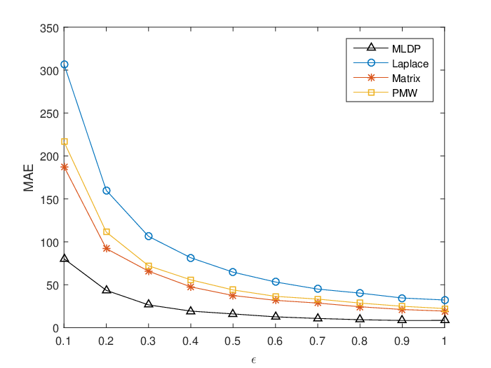
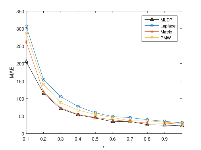
Apart from the traditional Laplace mechanism, we also compare MLDP with other two prevalent methods. The first is Matrix [12], which aims to decrease the correlation between batches of queries. The second is PMW [7]. It is one of the most populate iterative publishing methods in the differential privacy community. As both algorithms can only deal with count or range queries, we only test range queries with from to .
As shown in Fig. 5, we observe that MLDP has a lower MAE on all values of in all datasets. For example, in Fig. 5a, when , MLDP has an MAE of while the Laplace method has , with an improvement of . When , MLDP achieves an MAE of and outperforms Laplace which has . These results imply that MLDP outperforms traditional Laplace when answering a large set of queries. When compared with other methods, MLDP still has lower MAEs. When , the PMW has a MAE of and Matrix has a MAE of , which is higher than MLDP. This trend is consistent with the increase in . When reaches , PMW is and Matrix is , both of which are higher than that of MLDP with MAE.
The improvement achieved by MLDP can also be observed in Fig. 5b, 5c, and Fig. 5d. The proposed MLDP mechanism has better performance because the prediction process for answering test queries does not consume any privacy budget, while noise is only added in the training queries. The traditional Laplace method consumes the privacy budget when answering every query in the test set, and the sensitivity is affected by the correlation between large sets of queries, which leads to inaccurate answers. The experimental results show the effectiveness of MLDP in answering a large set of queries. It is also worth noting that this test set is unknown by MLDP in the training process, but for PMW, Matrix and Laplace, it should be provided before publishing. This shows that MLDP can deal with unknown queries, while other methods cannot.
In the context of differential privacy, the privacy budget is a key parameter for determining the level of privacy. From Fig. 5, we can also check the impact of on the performance of MLDP. According to Dwork [3], or less would be suitable for privacy preservation purposes, and we follow this rule in our experiments. For a comprehensive investigation, we evaluate MLDP’s performance at various privacy preservation levels, by varying the privacy budget from to with a step on four datasets. It is observed that as increases, the MAE evaluation becomes better, which means that the lower the privacy preservation level, the better the utility. In Fig. 5b, the MAE of MLDP is when . Even though it preserves a strict privacy guarantee, the query answer is inaccurate. When , the MAE drops to , retaining an acceptable utility in the result. The same trend can be observed on other datasets. For example, when , the MAE is in Fig. 5c, and is in Fig. 5d. Both show great improvement compared to . These results confirm that the utility is enhanced as the privacy budget increases.
We observe that the MAE decreases faster when ascends from to , than when ascends from to . This indicates that a larger utility cost is needed to achieve a higher privacy level (). We also observe that MLDP and other methods perform stably when . This indicates that MLDP is capable of retaining the utility for data release while satisfying a suitable privacy preservation requirement.
The evaluation shows the effectiveness of the MLDP method from several aspects. 1) It retains a higher accuracy compared to other methods when answering large sets of queries. 2) Its performance is significantly enhanced with the increase in the privacy budget. We can select a suitable privacy budget to achieve a better trade-off. 3) With a sufficient privacy budget, the utility loss can be trivial.


VI Related Work
A plethora of methods has been proposed for differentially private data publishing. Among them, two different types of method exist that preserve differential privacy for non-interactive data publishing. One type of method is synthetic dataset publishing another type is the batch queries publishing.
Synthetic dataset publishing attempts to publish a perturbed dataset instead of the original one. Mohammed et al. [13] proposed an anonymized algorithm DiffGen to preserve privacy for data mining purposes. The anonymization process satisfies the constraint of differential privacy. Zhang et al. [16] assumed that there are correlations between attributes. If these correlations can be modeled, the model can be used to generate a set of marginals to simulate the distribution of the original dataset. Chen et al. [2] addressed the similar problem by proposing a clustering generated method. All of above works are focusing on the dataset perturbation, there is another line of works concerning on the sampling method based on the learning theory.
With the learning theory development, Kasiviswanathan [10] claimed that almost anything learnable can be learned privately. Blum et al. [1] subsequently claimed that the main purpose of analyzing a dataset is to obtain information about a certain concept. Based on their theories, Kasiviswanathan et al. [10] proposed an Exponential-based mechanism to search a synthetic dataset from the data universe that is able to accurately answer a group of queries. Blum et al. [1] applied a similar Exponential-based mechanism, Net mechanism, to generate a synthetic dataset over a discrete domain.
Another type of method is to release a batch of queries instead of a dataset. The traditional Laplace method belongs to this type, but it introduces a large amount of noise due to the correlation between queries. Current research works focus on how to decrease the correlation between batches of queries, so that the total sensitivity can be diminished.
Xiao et al. [14] proposed a wavelet transformation, called Privelet, on the dataset to decrease the sensitivity. Li et al. [12] proposed the Matrix mechanism which answer sets of linear counting queries. Given a set of queries, the Matrix mechanism defines a workload accordingly and obtains noisy answers by implementing the Laplace mechanism. The estimates are then used on the to generate estimates of the submitted queries. Huang et al. [9] transformed the query sets to a set of orthogonal queries to reduce the correlation between queries. The correlation reduction helps to decrease the sensitivity of the query set. Yuan et al. [15] presented a low-rank mechanism (LRM), an optimization framework that minimizes the overall error of the results for a batch of linear queries.
The method in this paper is neither similar to synthetic dataset publishing, nor to batch query publishing. The proposed method aims to publish a model rather than a synthetic dataset or query answers. Unlike previous work, our work aims to publish a model to answer fresh queries. It is entirely new thinking on the data publishing problem which transfers data publishing into a machine learning process. Many challenges in non-interactive data publishing can thus be overcome by using existing flourishing machine learning theories.
VII Conclusions
Differential privacy is an influential notion in the research of privacy preserving data publishing, but the existing differentially private method fails to provide accurate results for publishing large numbers of queries. Two challenges must be tackled in this process: how to decrease the correlation between queries and how to deal with unknown queries before publishing. This paper proposes a query learning solution to deal with both challenges and makes the following contributions: We propose a novel MLDP method to transfer the data publishing problem to a machine learning problem and prove the accuracy bound of the MLDP. The MLDP method exploits a possible way to publish data structures. Extensive experiments has been used on both real and synthetic datasets to prove the effectiveness of the proposed MLDP. These contributions not only form a practical solution for non-interactive data publishing in terms of higher accuracy, but also propose a possible way to release various types of data in the future.
References
- [1] Avrim Blum, Katrina Ligett, and Aaron Roth. A learning theory approach to non-interactive database privacy. STOC, 2008.
- [2] Rui Chen, Qian Xiao, Yu Zhang, and Jianliang Xu. Differentially private high-dimensional data publication via sampling-based inference. In SIGKDD, 2015.
- [3] Cynthia Dwork. Differential privacy: a survey of results. In TAMC’08, pages 1–19, Berlin, Heidelberg, 2008. Springer-Verlag.
- [4] Cynthia Dwork. Differential privacy in new settings. In SODA ’10, 2010.
- [5] Cynthia Dwork. A firm foundation for private data analysis. Commun. ACM, 2011.
- [6] Cynthia Dwork, Vitaly Feldman, Moritz Hardt, Toniann Pitassi, Omer Reingold, and Aaron Leon Roth. Preserving statistical validity in adaptive data analysis. STOC, 2015.
- [7] Moritz Hardt and Guy N. Rothblum. A multiplicative weights mechanism for privacy-preserving data analysis. In FOCS 2010.
- [8] Michael Hay, Vibhor Rastogi, Gerome Miklau, and Dan Suciu. Boosting the accuracy of differentially private histograms through consistency. PVLDB, 2010.
- [9] Dong Huang, Shuguo Han, Xiaoli Li, and Philip S. Yu. Orthogonal mechanism for answering batch queries with differential privacy. SSDBM ’15, 2015.
- [10] Shiva Prasad Kasiviswanathan, Homin K. Lee, Kobbi Nissim, Sofya Raskhodnikova, and Adam Smith. What can we learn privately? In FOCS 2008.
- [11] Michael Kearns. Efficient noise-tolerant learning from statistical queries. J. ACM, 45:983–1006, 1998.
- [12] Chao Li and Gerome Miklau. Optimal error of query sets under the differentially-private matrix mechanism. ICDT ’13, pages 272–283, New York, NY, USA, 2013. ACM.
- [13] Noman Mohammed, Rui Chen, Benjamin C.M. Fung, and Philip S. Yu. Differentially private data release for data mining. KDD ’11, 2011.
- [14] Xiaokui Xiao, Guozhang Wang, and Johannes Gehrke. Differential privacy via wavelet transforms. IEEE Trans. on Knowl. and Data Eng., 2011.
- [15] Ganzhao Yuan, Zhenjie Zhang, Marianne Winslett, Xiaokui Xiao, Yin Yang, and Zhifeng Hao. Optimizing batch linear queries under exact and approximate differential privacy. ACM Trans. Database Syst., 2015.
- [16] Jun Zhang, Graham Cormode, Cecilia M. Procopiuc, Divesh Srivastava, and Xiaokui Xiao. Privbayes: private data release via bayesian networks. In SIGMOD 2014.
- [17] Tianqing Zhu, Gang Li, Wanlei Zhou, Ping Xiong, and Philip S. Yu. Differentially private data publishing and analysis: A survey. IEEE Transactions on Knowledge and Data Engineering, 29(8):1619–1638, Aug 2017.