Equation of State in 2+1 Flavor QCD at High Temperatures
Abstract
We calculate the Equation of State at high temperatures in 2+1 flavor QCD using the highly improved staggered quark (HISQ) action. We study the lattice spacing dependence of the pressure at high temperatures using lattices with temporal extent and and perform continuum extrapolations. We also give a continuum estimate for the Equation of State up to temperatures GeV, which are then compared with results of the weak-coupling calculations. We find a reasonably good agreement with the weak-coupling calculations at the highest temperatures.
pacs
12.38.Gc, 12.38.-t, 12.38.Bx, 12.38.MhI Introduction
Over the last several years there was a focused effort to calculate the Equation of State of strongly interacting matter at net zero baryon density in lattice QCD using physical or nearly physical quark masses and improved staggered action [1, 2, 3, 4, 5, 6, 7, 8]. As the result the continuum extrapolated Equation of State (EoS) has been obtained in 2+1 flavor QCD for physical light and strange quark masses [7, 8]. The calculations have been performed using two different improved staggered discretization schemes, the so-called stout action and the highly improved staggered quark (HISQ) action. These calculations cover a temperature range up to MeV. Overall the results of these calculations agree well, except for the highest temperatures, where tension between the two results can be seen [8]. It is important to clarify if this tension is just due to some statistical fluctuations or part of a systematic trend. Furthermore, for the comparison with the weak-coupling results it is highly desirable to extend the EoS calculations to higher temperatures. At temperatures MeV the charm quark contributes significantly to thermodynamic quantities and has to be included in the calculations [9]. Thus, one has to perform the calculations of the EoS in 2+1+1 flavor QCD. However, in the weak-coupling calculations the inclusion of the charm quark complicates the analysis, and the effects of the charm quark on the thermodynamic quantities are only known up to next-to-leading order (NLO) [10]. Also it is more difficult to control the discretization effects in the presence of the charm quark due to its large mass. Therefore, for comparison of the lattice QCD results and the weak-coupling results it is advantageous to consider thermodynamic quantities in 2+1 flavor QCD at higher temperatures. Such calculations also provide a solid reference point for estimating the charm quark contribution to QCD thermodynamics.
The purpose of this work is to extend the calculations presented in Ref. [8] to higher temperatures. As in Ref. [8] the HISQ action will be used together with the physical value of the strange quark mass. The lattice spacing (cutoff) dependence of the pressure will be studied in detail. In the previous studies the continuum extrapolations have been performed for the trace anomaly; the pressure and other thermodynamic properties have been obtained from the trace anomaly using the integral method [11]. The cutoff dependence of the trace anomaly, however, is expected to be more complicated than the cutoff dependence of the pressure. The reason for this is the following. In the weak-coupling picture the trace anomaly receives contributions starting at three loop, i.e. at order . Therefore, the understanding of the cutoff dependence of the trace anomaly at high temperature would in principle require a three-loop calculation in lattice perturbation theory. This is clearly formidable task. On the other hand the pressure at high temperature receives the leading contribution at one loop () corresponding to the ideal gas limit. Therefore, the cutoff dependence of the pressure at high temperature is known and to fairly good approximation is described by the free gas [12, 13].
For better understanding of the cutoff dependence of the EoS at high temperatures and a better control of the continuum extrapolation it is desirable to study the cutoff dependence of the pressure directly. This may also help to understand the difference between the continuum-extrapolated results and the results obtained with p4 or asqtad-improved staggered actions and and at high temperatures [3, 4] since cutoff effects here should be small.
It is expected that thermodynamic properties are not sensitive to the value of the light quark masses at high temperatures. The quark mass dependence of the EoS was studied in Ref. [6] and it was found that for light quark masses smaller than the quark mass dependence is very small for MeV. Therefore, we consider light quark masses which are five times smaller than the strange quark mass, , instead of the physical value. This choice of the light quark mass corresponds to a pion mass of about MeV in the continuum limit.
The rest of the paper is organized as follows. In Section II we discuss details of the lattice calculations. In Section III we show our results for the trace anomaly. In Section IV we present the calculation of the pressure and its cutoff dependence. Comparison of the lattice calculations to the weak-coupling results is discussed in Section V. Finally Section VI contains our conclusions. Some technical aspects of the calculations are presented in the appendices.
II Lattice calculations at zero temperature
The goal of this paper is to extend the calculations of the QCD Equation of State in Ref. [8] to higher temperatures. Therefore, as in Ref. [8] we use tree-level improved gauge action and HISQ action for quarks. To calculate the EoS gauge configurations at zero temperature had to be generated to perform the subtraction of the UV divergences in the thermodynamic quantities as well for the determination of the lattice spacing. We generated the gauge configurations at using the rational hybrid Monte-Carlo (RHMC) algorithm at five values of the lattice gauge coupling . The parameters of the simulations are shown in Tab. 1, including the lattice volume. The lowest two values will be used for the purpose of comparison with the previous 2+1 flavor results at smaller light quark masses [8], enabling us to quantify the quark mass effects in the scale setting procedure as well as in the thermodynamic quantities.
| vol | a [fm] | # traj. | ||
|---|---|---|---|---|
| 7.030 | 0.03560 | 0.08253 | 1890 | |
| 7.825 | 0.01542 | 0.04036 | 1265 | |
| 8.000 | 0.01299 | 0.03469 | 3927 | |
| 8.200 | 0.01071 | 0.02924 | 3927 | |
| 8.400 | 0.00887 | 0.02467 | 3927 |
The lattice spacings corresponding to the highest three values in Tab. 1 are smaller than fm. At these small lattice spacings it is expected that the Monte-Carlo (MC) evolution of the topological charge will effectively freeze. Indeed, we observe that the topological charge does not change in the MC evolution. To deal with this problem we generated MC streams corresponding to different values of topological charge, namely and . We checked whether the observables of interest are sensitive to the value of the topological charge, but we did not find any sensitivity. The dependence of different observables on the topological charge is discussed in Appendix A.
To determine the lattice spacing we calculated the static quark anti-quark potential. The lattice spacing is determined through the scale parameters and defined as
| (1) |
The parameter is widely used by the MILC and HotQCD collaborations to set the lattice spacing (see e.g. Ref. [8]). The value of this parameter is fm [14]. Since we consider smaller lattice spacings it is useful to consider the scale parameter . The calculation of the static potential and the determination of and scales is discussed in Appendix A.
For the two lower values in Tab. 1 we could compare the results on the static potential calculated for with the previous calculations performed at to study quark mass effects. We find no quark mass effects at the shortest distances. Quark mass effects increase with increasing distances but are less then for . At distances around the statistical errors in the static potential are large enough so that no quark mass effects in the derivative of the potential can be seen. Therefore, we can combine the newly determined values of with the previously published HotQCD results to obtain as function of . The details of this analysis are given in Appendix A.
III The QCD trace anomaly


To extend the calculation of the Equation of State of 2+1 flavor QCD we used the integral method, which relies on the calculation of the trace of the energy momentum tensor or the trace anomaly for short [3, 4]. The pressure can be calculated in terms of the trace anomaly as follows:
| (2) |
where is some reference temperature, which is sufficiently small, so can be either set to zero or taken from the hadron resonance gas calculation [3, 4, 8]. The trace anomaly can be expressed in terms of the expectation values of the gauge action, , and the light, , and strange, , quark condensates, calculated at finite and zero temperature, respectively. For the HISQ action the corresponding formula has the form [8]:
| (3) | ||||
| (4) | ||||
| (5) |
Here we used the same notation as in Ref. [8] and we made explicit the separation of the trace anomaly into the fermionic and gluonic parts. Furthermore, we introduced the nonperturbative beta function and mass renormalization function defined as [3, 4]
| (6) | ||||
| (7) |
The calculation of the nonperturbative beta function is discussed in Appendix A. The mass renormalization function is taken from Ref. [8]. As also discussed in Appendix A, the new zero temperature calculations are consistent with this mass renormalization function.
To calculate the trace anomaly at temperatures corresponding to the values of given in Table 1 we use the finite temperature gauge configurations from the TUMQCD collaboration [15, 16]. These gauge configurations have been generated on lattices with and and . The maximal temperature corresponding to these lattices is about GeV.
Now we will discuss our numerical results on the trace anomaly, in particular, its dependence on the light quark masses. There are two sources of quark mass dependence of the trace anomaly. First, is the dependence of the trace anomaly on the light sea quark masses. The second is the explicit dependence of the fermionic part of the trace anomaly on the light quark mass. As we will see later there are also differences in the cutoff () dependence of the fermionic and gluonic parts of the trace anomaly. Therefore, in the following we will discuss the numerical results for and separately. The fermionic part of the trace anomaly, is shown in Fig. 1 (left) and compared with the published HotQCD results obtained for [8] and shown as open symbols. To take into account the explicit dependence on the light quark masses in the calculation of we used the value instead of . We see from the figure that after adjusting the light quark mass there is no quark mass dependence in for MeV, i.e. the the quark mass dependence of due to the sea quarks is very small. From Fig. 1 (left) we also see that the cutoff effects in are very small in accordance with the previous study [8]. Finally, we note that statistical errors for are tiny. Our results for the gluonic part of the trace anomaly, , are shown in Fig. 1(right). The cutoff and quark mass dependence of can be clearly seen. The quark mass dependence of is due to the sea quarks and thus cannot be corrected. It is the sole source of the quark mass dependence of the trace anomaly shown in Fig. 2. We see, however, that quark mass effects become smaller at high temperatures and statistically are not significant for MeV. The statistical errors for are much larger than for and it is the dominant contribution to the trace anomaly.

For the calculation of the trace anomaly at high temperatures we also used lattices from the TUMQCD collaboration obtained with [15] and [16]. Our results for the trace anomaly at high temperatures are summarized in Fig. 2. The open symbols in the figure refer to results, while the filled symbols refer to results. All the results for are from Ref. [8], except the ones for and those for with or . ¿From Fig. 2 we see that results smoothly match to the results at high temperatures. This is expected. From the calculations of the trace anomaly performed with stout action at several quark masses we can estimate that the difference in the trace anomaly calculated for and is and for and MeV, respectively. Our calculations with at MeV confirm these expectations. The statistical errors shown in Fig. 2 are much larger than the above differences in the temperature range of interest, so no quark mass effects are visible given the errors. In Fig. 2 we also show the trace anomaly calculated with p4 action for and [3]. The corresponding results agree well with the HISQ results. Overall we see that quark mass effects are very small at high temperatures and therefore it is justified to study QCD thermodynamics with in this region. Finally, we note that there is no visible cutoff dependence for for in the high temperature region, while the and data are systematically below the results.

While the main purpose of this work is to extend the EoS calculations to high temperatures we also revisited the trace anomaly in the low temperature region for using the gauge configurations generated by the TUMQCD collaboration for the study of the Polyakov loop [15]. The reason behind this is the fact that unlike in Ref. [8] the continuum extrapolations will be performed in terms of the pressure and not the trace anomaly. Therefore, a more accurate determination of the pressure and the trace anomaly at low temperatures is needed. We added the following temperatures: MeV (), and MeV and MeV (). The gauge configurations are the same as in Ref. [8]. The numerical results for the trace anomaly in the low temperature region are shown in Fig. 3. We performed interpolations of the lattice results on using smoothing splines. The number of knots in the spline and the value of the smoothing parameter have been adjusted such that we obtain a smooth behavior with minimum number of knots and keep the close to one. The statistical error on the spline has been estimated using bootstrap method. We see sizable differences in calculated with and , indicating residual cutoff effects in the region MeV MeV. We also compare our results with the hadron resonance gas (HRG) model. We show two versions of the HRG model: one that takes into account all states from the particle data group, which we label as HRG-PDG, and one that includes baryon states that are not yet discovered experimentally, but predicted by the quark model (missing states). We label the latter model as HRG-QM. The details of the HRG models are described in Appendix B. There we also introduce the HRG-QM models for non-zero lattice spacing in addition to the continuum HRG-QM model shown in 3. ¿From the figure we see that the difference between the two HRG models is only significant for MeV. The lattice results for and agree with the HRG models only for MeV. This is in agreement with the previous results [7, 8]. Unlike in Ref. [8] we did not require that the interpolations agree with the HRG model at low temperatures. So these results serve as independent check for the validity of the HRG model.
IV The pressure of 2+1 flavor QCD from low to high temperatures
In this section we discuss the calculation of the pressure in the wide temperature range from MeV to MeV. For this purpose we combine the published HotQCD results for the trace anomaly with the results obtained for and discussed in the previous section. We use the published HotQCD results for MeV and , MeV and , MeV and , and MeV and [8]. For temperatures higher than these we use the new results with and . Since the quark mass effects are smaller than the statistical errors we treat these two data sets as one and perform interpolations of the data from the combined set. Using the resulting interpolating function we can calculate the pressure according to Eq. (2). Essentially we will be computing the pressure for lines of constant physics corresponding to even though the data for the trace anomaly at the high temperatures come from calculations at . To fix the pressure completely we need to specify the lower integration limit as well as the value of the pressure at . The lower integration limit is determined by the lowest data point for which a lattice calculation of is available for given . As in Ref. [8] we will use HRG to estimate the pressure at . However, when choosing the value of we need to take into account the discretization effects of the staggered fermion formulation due to the distortion of the hadron spectrum. Therefore we calculate in the HRG model with distorted hadron spectrum. The details of these calculations are discussed in Appendix B. As the result we obtain a value for each . The values of and used in the calculation of the pressure are given in Table 2.


| [MeV] | ||
|---|---|---|
| 6 | 135 | 0.189(54) |
| 8 | 120 | 0.145(22) |
| 10 | 125 | 0.226(23) |
| 12 | 135 | 0.344(29) |
With these inputs we can calculate the pressure for and . The results are shown in Fig. 4. We see significant cutoff dependence in the low temperature region and smaller cutoff dependence in the high temperature region. In the low temperature region the pressure follows qualitatively the cutoff dependence obtained in the HRG model with distorted hadron spectrum, cf. Fig. 4 (left). The continuum limit for the pressure is approached from below. The pressure shows stronger cutoff dependence than the trace anomaly. Both of these features could be understood in the framework of the HRG model with distorted hadron spectrum (see Appendix B).

At high temperatures the cutoff dependence of the pressure can be understood in the weak-coupling picture. In this picture the pressure can be written as the sum of quark and gluon pressures with the latter being defined as the QCD pressure for 11 1 Note that this decomposition of the pressure into the quark and gluon pressures is different from the decomposition of into and . The quark pressure does not vanish for zero quark mass but does.. The cutoff dependence of the quark and gluon pressures has been studied in lattice perturbation theory up to order [17, 13, 18]. To a good approximation this cutoff dependence is described by the ideal gas result. The cutoff dependence of the gluon pressure is very small () for if improved gauge action is used [12]. This is confirmed by direct lattice numerical study [17]. Therefore we neglect it here. The cutoff dependence of the quark pressure was studied in Refs. [13, 18] for improved staggered actions, namely the Naik action and p4 action. The cutoff dependence of the quark pressure is much bigger than of the gluon pressure for . At tree level the HISQ action has the same cutoff dependence as the Naik action. Thus, the ideal gas limit for the HISQ action is determined by the result for Ref. [13]. The ideal gas limit for each is shown in Fig. 4 as a horizontal line. Our numerical results for the pressure at high temperatures shown in Fig. 4 (right) follow the same trend in terms of cutoff dependence as the free theory result. The result appears to be an exception, though given the statistical errors the deviations from the trend is not very significant. At quantitative level the cutoff effects in the pressure are smaller than in the free field theory. This observation is in line with the cutoff dependence of the pressure in SU(3) gauge theory [11] as well as cutoff effects of quark number susceptibilities (QNS) obtained with HISQ action [19, 20]. For comparison we also show the pressure obtained with p4 action and or lattices [3, 4]. The corresponding results are significantly larger than the ones obtained with HISQ action at high temperatures and significantly lower at small temperatures. This is most likely due to the large cutoff effects related to taste-symmetry breaking for the p4 action (see discussions in Appendix B).
The cutoff dependence of the pressure obtained with HISQ action and p4 action closely resembles the cutoff dependence of quark number susceptibilities (QNS) defined as second and fourth derivatives of the pressure with respect to quark chemical potential,
| (8) |
Since the cutoff dependence of the quark contribution to the pressure and the cutoff dependence of QNS are similar, we could use the latter to correct for the cutoff dependence of the former. This can be done as follows. We write the pressure as the sum of the quark and gluon pressures22 2 This can be done if the weak-coupling picture holds at high temperatures, as expected. . Assuming that the gluonic pressure has negligible cutoff dependence (see the above discussions) we can write
| (9) |
where is the pressure at fixed lattice spacing () and
| (10) |
is the correction factor due to discretization errors. Here stands for the quark pressure in the continuum limit, while is the quark pressure at non-zero lattice spacing, . If we assume that the cutoff dependence of the quark pressure is the same as of the second order QNS, , i.e.
| (11) |
we can use the results of Ref. [19] to obtain the correction provided we also have an estimate for continuum quark pressure . Lattice calculations show that the QCD pressure is below the ideal gas limit by about at high temperatures. Therefore, the ideal quark pressure provides a fair estimate for . Thus, we have an estimate for the correction. We apply this correction to the pressure calculated for fixed . The results are shown in Fig. 5. We see from the figure that the pressure bands corresponding to different agree within errors, i.e. applying the corrections largely reduces the dependence of the results. We also see that while the p4 results are still higher than the HISQ results they agree within the statistical errors of the latter. The cutoff dependence of the pressure is understood because to a fairly good approximation it is given by the cutoff dependence of the free quark gas. This is not the case for the cutoff dependence trace anomaly, which would require a three-loop calculation as mentioned in Section I.


Now, that the cutoff dependence of the pressure is understood we can proceed with the continuum extrapolations. As discussed above at high temperatures the dominant cutoff dependence of the pressure is given by the cutoff dependence of the ideal quark gas, and therefore, for improved staggered actions like HISQ it is expected to scale like . This expectation is confirmed by the study of QNS at high temperatures with HISQ action [19, 20]. On the other hand at low temperatures the dominant cutoff effects are due to taste-symmetry breaking of staggered fermions and scale like . This is also confirmed by lattice calculations [21]. We find that the cutoff dependence of the pressure is incompatible with behavior for MeV. Similar findings have been obtained for QNS [19, 20]. On the other hand, for MeV we find that behavior of the cutoff effects is incompatible with the data. Therefore, we will assume that the cutoff effects are proportional to , when performing continuum extrapolations for MeV. In the intermediate temperature region, the cutoff effects should be proportional to some combination of and . Thus, one should in principle fit the data by form to obtain the continuum limit. But because we have only four values and the errors of the and data are large the continuum result obtained from such fits has large statistical error. It turns out, however, that in this intermediate temperature region it is possible to fit the cutoff dependence of the pressure with form as well as with form and obtain . The fits give higher values of the pressure than the fits, though the results from both fits overlap within the error bands. The difference between the central values of the and fits could be considered as a measure of the systematic error of the continuum extrapolation. This difference turns out to be about the same as the statistical errors of the extrapolations. Therefore, we estimate the total error of the continuum pressure for by doubling the statistical error of the fit. Alternatively we could add the systematic error estimated as described above with the statistical error in quadrature to obtain the total error. The corresponding errors will be smaller. We prefer to be more conservative. Similar analysis as above has been performed to obtain the continuum extrapolated result for the entropy density.
In the temperature interval MeV MeV we have four lattice spacings to perform continuum extrapolations. As the result the continuum extrapolations are most reliable in this temperature interval. In the temperature range MeV MeV we have three lattice spacings, so controlled continuum extrapolation is still possible. For MeV, we can only provide a continuum estimate for the pressure. For MeV we do this by performing fit of the and data for the pressure. Interestingly, it turns out that the coefficient of obtained when using only and data, and when using and data is the same within errors for MeV. So perhaps this extrapolation is not totally out of control. Finally, to obtain the continuum estimate for MeV we assume that the coefficient of the term is the same as obtained from the fit of the and data at MeV and correct the pressure by times this coefficient. The continuum results for the pressure obtained using this procedure are shown in Fig. 5 and compared to the corrected results for and . The continuum result for the pressure agrees with the corrected results. This serves as an important cross-check for our continuum extrapolations for MeV.


.
For comparison of the lattice calculation of the EoS with the weak-coupling results it is important to have an alternative method to obtain continuum results for MeV and also extend the calculation to higher temperatures. In order to do this we consider again the trace anomaly. As discussed in Section III for and MeV we do not see any cutoff dependence of the trace anomaly. This also means that given the statistical errors the results for the trace anomaly can be considered as the continuum ones. Therefore, we can perform a combined interpolation of the numerical results for the trace anomaly obtained with and in the temperature interval MeV MeV, providing a continuum estimate. The and results for the trace anomaly lie below this continuum estimate. However, if we re-scale the and results on the trace anomaly by factors and , respectively, they agree with the above continuum estimate for MeV MeV within errors. This is demonstrated in Fig. 6. Therefore, to obtain a continuum estimate for the trace anomaly beyond MeV we re-scale the and data for MeV with the above factors. Here we tacitly assume that the cutoff dependence of the trace anomaly is temperature independent. This assumption, however, is quite reasonable since the cutoff dependence at high temperatures should be described by weak-coupling expansion and thus is proportional to times the coupling constant to some power. Since the coupling constant depends on the temperature scale logarithmically in a limited temperature interval the cutoff effects should be approximately temperature independent. Our study of the dependence of the pressure for MeV confirms this expectation. The cutoff dependence of the quark number susceptibilities [19, 20] and the free energy of the static quark [15] also support this assumption. Therefore, we perform a spline interpolation of the combined and data in the temperature interval MeV MeV. Because we corrected the trace anomaly obtained on and lattices we assign an additional systematic error of and to the corresponding data points before the interpolation, i.e. the size of the systematic errors that we assume is the same as the magnitude of the correction. Using this interpolation we calculate the integral of the trace anomaly from MeV to MeV, which together with the continuum result for the pressure at MeV obtained above gives us the continuum pressure estimate that extends to temperatures as high as MeV. From the pressure we can also calculate the entropy density. These calculations will be used in the next section for the comparison with the weak-coupling results. We also compared this continuum estimate of the pressure with the one discussed before. For MeV we find excellent agreement between the two continuum estimates.
We note that our continuum result for MeV is one and a half sigma higher than the continuum result of Ref. [7], while our continuum estimate for higher temperatures is higher than the continuum estimate of Ref. [6]. Our continuum result for the pressure for MeV agrees very well with the HotQCD result [8] but has considerably smaller errors.
V Equation of state at high temperatures and comparison with weak-coupling calculations
In this section we compare the lattice results on the EoS with the weak-coupling calculations. We start our discussion with the trace anomaly. In Fig. 7 we compare our lattice results for the trace anomaly obtained with and as well as the corrected results for and (see previous section) with the results of three-loop HTL perturbation theory [22]. We see good agreement between the lattice results and the results obtained in three-loop HTL perturbation theory, although the error band of the latter is still quite large. The lattice results on the trace anomaly agree very well with the weak-coupling calculations based on dimensionally reduced effective field theory, the electrostatic QCD (EQCD) [10].
Next we compare the high temperature lattice results for the pressure and the entropy density with the three-loop HTL perturbation theory [22] and the results obtained using EQCD [10]. The comparison is shown in Fig. 8. For MeV we use the continuum extrapolated lattice results obtained from the calculations on and lattices. For higher temperatures, we use the continuum estimate based on the trace anomaly calculated on the coarsest lattice. As discussed in the previous section this continuum estimate is validated by direct continuum extrapolation for MeV, but at higher temperatures it relies on the temperature independence of the cutoff effects. Therefore, in Fig. 8 we show the continuum estimate as open symbols. We see that the EQCD calculations are higher than our lattice results. Our lattice results lie above the central value of the three-loop HTL perturbative result by one sigma. However, the lattice data are fully contained within the uncertainty of the three loop HTL result. In the considered temperature range the uncertainty of the lattice results is significantly smaller than the uncertainty of the three-loop HTL result. For the entropy density we also compare our lattice results with the resummed perturbative calculations in next-to-leading log approximation (NLA) [23]. This comparison is shown in Fig. 8 (right). The NLA calculation leads to higher entropy density than the lattice result, although overlaps within the uncertainty with latter for MeV. The NLA calculation is based on the derivable approach [24, 25, 26]. In this approach one calculates the derivatives of the pressure, which leads to cancellation of many higher order diagrams. As the result one obtains relatively simple expressions for the entropy density [26] or the quark number susceptibility [27]. The calculation of the pressure in this approach, however, is difficult.
It is clear that our lattice results are sufficiently precise to test the various weak-coupling approaches and it would be desirable to further reduce the uncertainty of the weak-coupling approaches to see if the thermodynamics of the quark gluon plasma can be indeed understood using the weak-coupling expansion in the considered temperature range.
VI Conclusions
We extended the previous calculation of the EoS with HISQ action to higher temperatures. First, we extended the calculation of the trace anomaly to higher temperatures using lattice simulations at larger quark mass, . We showed that the quark mass dependence of the trace anomaly is negligible for MeV given the statistical error. Then using the results on the trace anomaly and the integral method we calculated the pressure for and . We studied the cutoff () dependence of the pressure and performed the continuum extrapolation in the high temperature limit. We pointed out that the cutoff dependence of the pressure is dominated by the quark contribution and the cutoff dependence of this contribution is very similar to the cutoff dependence of QNS at high temperatures. We also showed that using the known cutoff dependence of QNS it is possible to correct for the cutoff effects in the pressure at fixed . The corrected results for the pressure calculated with HISQ action and p4 action for different agree within errors and also agree with the continuum result. Thus, we achieved a controlled continuum extrapolation of the pressure at high temperatures. Finally, using and results on the trace anomaly we provided a continuum estimate for the pressure that extends to temperatures as high as MeV. We compared this continuum estimate with the weak-coupling calculations and found a reasonably good agreement between the lattice and the weak-coupling results.
Acknowledgements
The simulations have been carried out on the computing facilities of the Computational Center for Particle and Astrophysics (C2PAP), SuperMUC and NERSC. We used the publicly available MILC code to perform the numerical simulations [28]. The data analysis was performed using the R statistical package [29]. We thank F. Karsch for providing the numerical values of the free quark pressure for finite . We also thank M. Strickland and N. Haque for sending the 3-loop HTL results for the EoS. This work has been supported in part by the U.S Department of Energy through grant contract No. DE-SC0012704. J. H. Weber acknowledges the support by the Bundesministerium für Bildung und Forschung (BMBF) under grant “Verbundprojekt 05P2015 - ALICE at High Rate (BMBF-FSP 202) GEM-TPC Upgrade and Field theory based investigations of ALICE physics” under grant No. 05P15WOCA1.
Appendix A Zero temperature calculations
For and we generated a single stream of MC evolution. For the highest three values we generated three streams of MC evolution called a, b and c; each of these streams corresponds to a single value of topological charge . The lengths of these streams for every value of are , and , respectively. The values of the plaquette, rectangles, light and strange quark condensates are given in Tab. 3 together with the values of . The values of rectangles and plaquettes are the same within errors for the streams with different . For the quark condensate we see small, but in some cases statistically significant differences. The difference in the value of the light quark condensate is between and , while for the strange quark condensates it is . For there are differences in the values of the light quark condensate also for the streams that belong to the same topological sector, which appear to be statistically significant. This is most likely due to the fact that each of the streams is relatively short. These small differences, are taken into account in the calculations as additional systematic errors. However, the additional systematic effects are largely irrelevant for the calculation of the trace anomaly, since the highest three beta values correspond to temperatures MeV, where the contribution of quark condensates is very small.
| plaq. | rect. | Q | stream | |||
|---|---|---|---|---|---|---|
| 0.6641244(21) | 0.0026400(66) | 0.0117787(51) | 0.4607658(29) | 2 | a | |
| 8.0 | 0.6641256(15) | 0.0026061(122) | 0.0117719(76) | 0.4607666(23) | 1 | b |
| 0.6641257(24) | 0.0025923(87) | 0.0117889(59) | 0.4607666(35) | 0 | c | |
| 0.6738855(16) | 0.00207849(52) | 0.0095507(55) | 0.4744956(24) | 2 | a | |
| 8.2 | 0.6738854(12) | 0.00199916(69) | 0.0095271(60) | 0.4744943(17) | 0 | b |
| 0.6738865(12) | 0.00201003(95) | 0.0095399(75) | 0.4744971(18) | 0 | c | |
| 0.6830217(14) | 0.00171386(47) | 0.0078134(48) | 0.4874515(22) | 2 | a | |
| 8.4 | 0.6830200(17) | 0.00158675(57) | 0.0077629(71) | 0.4874514(28) | 0 | b |
| 0.6830187(12) | 0.00161808(63) | 0.0077963(54) | 0.4874474(18) | 0 | c |
.
To determine the lattice spacing we calculated the static quark anti-quark potential. We followed the same procedure as in Ref. [8], in particular the same fit ranges in time were used. For the highest three values we used a fit range in , which is about the same as in Ref. [8] for . Our results for the potential are shown in Fig. 9. We calculated the static quark anti-quark potential for different topological sectors and did not see any dependence on the topological charge within the statistical errors.
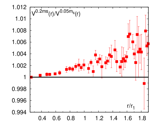
It is interesting to compare the potential calculated for and at the same value of . Such a comparison is shown in Fig. 10 for . As one can see from the figure the quark mass effects are very small for . They are the smallest at the shortest distance and gradually increase with increasing . However, even for the effects are smaller than and for are smaller than . We get very similar results for .

We also find that the difference between the potential calculated for and in units of can be parametrized as
| (12) |
We get for and for . ¿From these we can estimate that is changed by about around , and by about or less around , when changing from to . Therefore, we expect shifts in the values of and with changing quark masses, which are similar in magnitude.
The scale obtained from the potential at and is given in Tab. 4. For we also calculated the scale. Moreover, this scale was calculated for using the data on the potential from [8]. The results are given in Tab. 4. We see that the scale is about smaller for than for . This difference is consistent with the above expectations and statistically it is not very significant. The value of at is smaller for than for . Again this difference is statistically not significant. Since the scale shows smaller quark mass dependence we could use it to extend the scale setting procedure of Ref. [8] to higher , namely up to . To do this we first consider the ratio , which is shown in Fig. 11. We do not see any dependence of this ratio within errors.
| 8.400 | 1/5 | 12.560(130) | 5.742(31) |
|---|---|---|---|
| 8.200 | 1/5 | 10.653(60) | 4.861(36) |
| 8.000 | 1/5 | 8.905(60) | 4.075(30) |
| 7.825 | 1/5 | 7.570(104) | 3.469(18) |
| 7.825 | 1/20 | 7.690(58) | 3.479(21) |
| 7.596 | 1/20 | 6.336(56) | 2.865(11) |
| 7.373 | 1/20 | 5.172(34) | 2.350(40) |
| 7.030 | 1/5 | 3.737(13) | - |
| 7.030 | 1/20 | 3.763(13) | - |

Fitting we get , while the fit with we obtain . Finally the fits for all in the interval we get
| (13) |
which agrees with the above values within errors. Since is essentially mass independent and more accurately determined than for the highest values we will use it for the scale setting. We combine the results of Ref. [8] together with for and from Tab. 4 to obtain the lattice spacing in units of in the region that extends to . As in Ref. [8] we fit with an Allton-type form [30]:
| (14) | ||||
| (15) |
Here and are the well-known coefficients of the two-loop beta function, which for the three-flavor case read , . Fitting the combined data set for the coefficients and we get:
| (16) | ||||
| (17) | ||||
| (18) | ||||
| (19) |
The above errors have been estimated by bootstrap method and they are smaller than those in [8], in particular the error on is reduced from to . This fit is shown in Fig. 12 with the band indicating its uncertainty. The difference between this parametrization of and the one in Ref. [8] is less than in the entire range of . It is interesting to note that for the highest value the deviation from the asymptotic 2-loop result is only one sigma. ¿From this fit we can determine the smoothed value of for each value of and thus the temperature scale.


For the calculation of the EoS we also need the non-perturbative beta function defined as
| (20) |
Appendix B The hadron resonance gas and cutoff effects at low temperatures
In the HRG model the partition function of strongly interacting matter at low temperatures is given by the partition function of non-interacting hadrons and resonances
| (21) |
where
| (22) |
with energies and degeneracy factors . The superscripts and refer to mesons and baryons. Usually the sum in the above equation contains all the meson and baryons from the Particle Data Group (PDG). However, our information of the baryon spectrum may be incomplete. There are lots of baryon states predicted by the quark model (QM) [31] as well as by lattice QCD [32] that are not included in the PDG. These are the so-called missing states. It was shown that these missing states are important for QCD thermodynamics [33, 34, 35, 36, 37]. Therefore, we included these missing states in the HRG model. We used the baryon spectrum from the quark model calculations of Refs. [38, 39]. We call this model HRG-QM. For the strange baryons we also used the spectrum from Ref. [31] and found that this only results in very small differences relative to the above calculation. The difference between the HRG-QM and the HRG model which includes only hadrons from PDG, and therefore is called HRG-PDG, is visible only for MeV. At these temperatures, however, the HRG model itself may not be reliable.
The hadron resonance gas can be used as a tool to understand the cutoff effects in the EoS at low temperatures. Lattice discretization errors will modify the hadron spectrum which then leads to the modification of the HRG. This has been discussed in some details for p4 and asqtad actions [40]. Below we will discuss the discretization effects in the hadron spectrum for the HISQ action and their effect on thermodynamics of hadrons.
The staggered fermion formulation describes four flavors (tastes) of quarks in the continuum limit. To describe a single quark flavor one takes the fourth root of the staggered fermion determinant in the path integral of QCD. This is the so-called rooting trick and amounts to averaging over the four staggered tastes for each physical flavor. For the discussion of the cutoff effects on the hadron spectrum we first limit ourselves to the original four-flavor case. There are 16 pseudo-scalar (ps) mesons, which are the Goldstone bosons of the theory. At non-zero lattice spacing only a subgroup of the group is preserved, and there is only one Goldstone boson in the chiral limit. The other ps mesons have squared masses proportional to , . The breaking of the full chiral symmetry to a subgroup and the corresponding splitting of ps mesons is referred to as taste-symmetry breaking. It is the largest source of discretization errors in today’s lattice calculations with staggered fermions. The size of taste-symmetry breaking, i.e. the value of coefficients can be reduced by using improved actions. All improved staggered actions (p4, asqtad, stout and HISQ) reduce the size of taste-symmetry breaking to some degree, The HISQ action has the smallest taste-symmetry breaking among the improved staggered fermion actions [41]. The taste symmetry breaking effects are particularly large for the p4 action.
Taste-symmetry breaking also causes non-degeneracy of vector mesons and baryons that belong to different tastes. However, the corresponding mass splittings are much smaller than in the case of ps mesons. For the HISQ action they are of the size of statistical errors and therefore can be neglected in the following discussion. The dominant effects of taste-symmetry breaking in the vector meson and baryon sectors come from the fact that the calculations are effectively performed at larger value of the pion mass than the physical one if the lattice spacing is non-zero. Since hadronic quantities like hadron masses and decay constants decrease with decreasing pion masses, we expect that the continuum limit for these quantities is approached from above. The masses of the vector mesons, nucleons and baryons have been calculated with HISQ action for different lattice spacings [41, 8]. We complement these studies by also calculating the masses of octet baryons with strangeness and for corresponding to lattice spacing fm. In Fig. 14 we show the vector meson and baryon masses as function of the lattice spacing. We see that following our expectations the hadron masses approach their continuum limit from above. We fit the -dependence of the hadron masses by the form
| (23) |
The values of and are given in Table 5. The resulting fits are also shown in Fig. 14 as lines and describe the data fairly well. For and baryons we could not perform the above fits. We model their lattice spacing dependence using Eq. (23) with coefficients and obtained for the nucleon and divided by two and three, respectively. This seems to capture the cutoff effects in and , see Fig. 14.


To reduce cutoff effects in the thermodynamic quantities it has been suggested to use the kaon decay constant to set the lattice spacing. Since shows an -dependence that is similar to that of the hadron masses the ratios are expected to have much milder -dependence. As the consequence thermodynamic quantities will also have smaller cutoff dependence if is used to set the scale. We checked that the -dependence almost entirely disappears for and mesons, as well as for the baryon if is used to set the lattice spacing. However, for the nucleon and other baryons this is not the case. Furthermore, the large taste-symmetry breaking in the ps meson sector cannot be compensated by changing scale from to .
| 1.2138 | 0.259522 | 0.24377 | 1.85148 | 0.306749 | |
| 18.1236 | 0 | 0 | 5.42284 | 0 |
To take into account the effects taste-symmetry breaking in the ps meson sector the contributions of pions, kaons and eta mesons are calculated as [40]
| (24) |
where . The quadratic pseudo-scalar meson splittings have been calculated in Ref. [41]. The dependence of these splittings can be fitted well by the form
| (25) |
The value of the coefficients an together with the degeneracy factors are given in Table 6.
| i | 0 | 1 | 2 | 3 | 4 | 5 | 6 | 7 |
|---|---|---|---|---|---|---|---|---|
| 1 | 1 | 3 | 3 | 3 | 3 | 1 | 1 | |
| 0 | 8.34627 | 8.17699 | 14.6245 | 16.0450 | 21.1623 | 23.0067 | 30.8425 | |
| 0 | -4.83538 | -6.09594 | -6.72714 | -5.2249 | -6.47337 | -5.49115 | -3.64465 |
The contribution of the ground state vector mesons can be evaluated at non-zero lattice spacing using Eqs. (22) and (23) and the corresponding values of and from Table 5. The -dependence of the octet baryon masses, as well as of mass is fixed through Eq. (23) and the values of the coefficients are given in Table 5. To completely specify the contribution of the ground state baryons to the partition function we assume that the masses of the decuplet baryons for and have the same -dependence as their octet partners. Thus the contribution of all ground state hadrons at non-zero is now fixed.
We need to consider also the contributions from the excited mesons and baryons. Unfortunately not much is known about the cutoff dependence of the excited hadron states in the staggered fermion formulations. We will work with two extreme assumptions about the cutoff dependence of the excited hadron states. First, we will assume that the masses of excited hadron states are not affected by the lattice cutoff. Second, we will assume that the masses of the excited hadron states are affected by the lattice cutoff the same way as the masses of the corresponding ground state hadrons. Furthermore, we will calculate the EoS in the HRG model assuming that only ps mesons are affected by the taste-symmetry breaking. We will compare these three scenarios with the continuum HRG model in order to understand the size of the cutoff effects. We will use the HRG model with missing states (HRG-QM) in what follows. The trace anomaly calculated for different is shown in Fig. 15 and compared to the lattice results. In Fig. 16 we show the pressure calculated for the same set of values. We see that the difference between the continuum HRG and the lattice HRG is larger for the pressure than for the trace anomaly, and the continuum limit is approached from below. The difference in the cutoff dependence of the trace anomaly and the pressure can be understood as follows. The cutoff effects make the hadrons heavier. This reduces the pressure as expected. However, states with larger masses contribute more to the trace anomaly. So this partially compensates the exponential suppression due to larger quark masses in the case of the trace anomaly in the considered temperature range. At sufficiently low temperatures, the cutoff dependence of the pressure and the trace anomaly are qualitatively similar. We also note that the reduction of the pressure relative to the continuum HRG expectation is mostly due to the ps meson sector. As one can see from Fig. 16 taking into account the modification of the baryon and vector meson masses in the HRG calculations only results in relatively small effects. We also note that for p4 and asqtad actions the cutoff effects due to taste-symmetry breaking are much larger [40].


We use the value of the pressure in the modified HRG-QM, in which the cutoff dependence of all the ground state hadrons is taken into account as discussed above (middle curves in Fig. 16) to determine the pressure at some initial value of the temperature in the integral method (see Section IV). To estimate the uncertainty in we consider the difference between the HRG-QM model in which only ps mesons are modified (upper curves in Fig. 16) and the HRG-QM model in which all ground state and excited state hadrons are modified (lower curves in Fig. 16). The resulting values are given in Table 2.
References
- [1] Y. Aoki, Z. Fodor, S. D. Katz, and K. K. Szabo, JHEP 01, 089 (2006), arXiv:hep-lat/0510084 [hep-lat] .
- [2] C. Bernard, T. Burch, C. E. DeTar, S. Gottlieb, L. Levkova, U. M. Heller, J. E. Hetrick, R. Sugar, and D. Toussaint, Phys. Rev. D75, 094505 (2007), arXiv:hep-lat/0611031 [hep-lat] .
- [3] M. Cheng et al., Phys. Rev. D77, 014511 (2008), arXiv:0710.0354 [hep-lat] .
- [4] A. Bazavov et al., Phys. Rev. D80, 014504 (2009), arXiv:0903.4379 [hep-lat] .
- [5] M. Cheng et al., Phys. Rev. D81, 054504 (2010), arXiv:0911.2215 [hep-lat] .
- [6] S. Borsanyi, G. Endrodi, Z. Fodor, A. Jakovac, S. D. Katz, S. Krieg, C. Ratti, and K. K. Szabo, JHEP 11, 077 (2010), arXiv:1007.2580 [hep-lat] .
- [7] S. Borsanyi, Z. Fodor, C. Hoelbling, S. D. Katz, S. Krieg, and K. K. Szabo, Phys. Lett. B730, 99 (2014), arXiv:1309.5258 [hep-lat] .
- [8] A. Bazavov et al. (HotQCD), Phys. Rev. D90, 094503 (2014a), arXiv:1407.6387 [hep-lat] .
- [9] S. Borsanyi et al., Nature 539, 69 (2016), arXiv:1606.07494 [hep-lat] .
- [10] M. Laine and Y. Schroder, Phys. Rev. D73, 085009 (2006), arXiv:hep-ph/0603048 [hep-ph] .
- [11] G. Boyd, J. Engels, F. Karsch, E. Laermann, C. Legeland, M. Lutgemeier, and B. Petersson, Nucl. Phys. B469, 419 (1996), arXiv:hep-lat/9602007 [hep-lat] .
- [12] B. Beinlich, F. Karsch, and E. Laermann, Nucl. Phys. B462, 415 (1996), arXiv:hep-lat/9510031 [hep-lat] .
- [13] U. M. Heller, F. Karsch, and B. Sturm, Phys. Rev. D60, 114502 (1999), arXiv:hep-lat/9901010 [hep-lat] .
- [14] A. Bazavov et al. (MILC Collaboration), PoS LATTICE2010, 074 (2010), arXiv:1012.0868 [hep-lat] .
- [15] A. Bazavov, N. Brambilla, H. T. Ding, P. Petreczky, H. P. Schadler, A. Vairo, and J. H. Weber, Phys. Rev. D93, 114502 (2016), arXiv:1603.06637 [hep-lat] .
- [16] A. Bazavov, N. Brambilla, P. Petreczky, A. Vairo, and J. H. Weber, Color screening in 2+1 flavor QCD, TUM-EFT 81/16.
- [17] B. Beinlich, F. Karsch, E. Laermann, and A. Peikert, Eur. Phys. J. C6, 133 (1999), arXiv:hep-lat/9707023 [hep-lat] .
- [18] P. Hegde, F. Karsch, E. Laermann, and S. Shcheredin, Eur. Phys. J. C55, 423 (2008), arXiv:0801.4883 [hep-lat] .
- [19] A. Bazavov, H. T. Ding, P. Hegde, F. Karsch, C. Miao, S. Mukherjee, P. Petreczky, C. Schmidt, and A. Velytsky, Phys. Rev. D88, 094021 (2013), arXiv:1309.2317 [hep-lat] .
- [20] H. T. Ding, S. Mukherjee, H. Ohno, P. Petreczky, and H. P. Schadler, Phys. Rev. D92, 074043 (2015), arXiv:1507.06637 [hep-lat] .
- [21] A. Bazavov et al. (HotQCD), Phys. Rev. D86, 034509 (2012a), arXiv:1203.0784 [hep-lat] .
- [22] N. Haque, A. Bandyopadhyay, J. O. Andersen, M. G. Mustafa, M. Strickland, and N. Su, JHEP 05, 027 (2014), arXiv:1402.6907 [hep-ph] .
- [23] A. Rebhan, in Proceedings, 5th Internationa Conference on Strong and Electroweak Matter (SEWM 2002): Heidelberg, Germany, October 2-5, 2002 (2003) pp. 157–166, arXiv:hep-ph/0301130 [hep-ph] .
- [24] J. P. Blaizot, E. Iancu, and A. Rebhan, Phys. Rev. Lett. 83, 2906 (1999a), arXiv:hep-ph/9906340 [hep-ph] .
- [25] J. P. Blaizot, E. Iancu, and A. Rebhan, Phys. Lett. B470, 181 (1999b), arXiv:hep-ph/9910309 [hep-ph] .
- [26] J. P. Blaizot, E. Iancu, and A. Rebhan, Phys. Rev. D63, 065003 (2001a), arXiv:hep-ph/0005003 [hep-ph] .
- [27] J. P. Blaizot, E. Iancu, and A. Rebhan, Phys. Lett. B523, 143 (2001b), arXiv:hep-ph/0110369 [hep-ph] .
- [28] MILC code, http://www.physics.utah.edu/~detar/milc/.
- [29] R statistical package, http://www.r-project.org/.
- [30] C. R. Allton, Nucl. Phys. Proc. Suppl. 53, 867 (1997), arXiv:hep-lat/9610014 [hep-lat] .
- [31] S. Capstick and N. Isgur, Phys.Rev. D34, 2809 (1986).
- [32] R. G. Edwards, N. Mathur, D. G. Richards, and S. J. Wallace (Hadron Spectrum), Phys. Rev. D87, 054506 (2013), arXiv:1212.5236 [hep-ph] .
- [33] A. Majumder and B. Muller, Phys.Rev.Lett. 105, 252002 (2010), arXiv:1008.1747 [hep-ph] .
- [34] A. Bazavov et al., Phys. Rev. Lett. 113, 072001 (2014b), arXiv:1404.6511 [hep-lat] .
- [35] A. Bazavov et al., Phys. Lett. B737, 210 (2014c), arXiv:1404.4043 [hep-lat] .
- [36] A. Bazavov et al., Phys. Rev. D95, 054504 (2017a), arXiv:1701.04325 [hep-lat] .
- [37] A. Bazavov et al. (HotQCD), (2017b), arXiv:1708.04897 [hep-lat] .
- [38] U. Loring, B. C. Metsch, and H. R. Petry, Eur.Phys.J. A10, 395 (2001a), arXiv:hep-ph/0103289 [hep-ph] .
- [39] U. Loring, B. C. Metsch, and H. R. Petry, Eur.Phys.J. A10, 447 (2001b), arXiv:hep-ph/0103290 [hep-ph] .
- [40] P. Huovinen and P. Petreczky, Nucl. Phys. A837, 26 (2010), arXiv:0912.2541 [hep-ph] .
- [41] A. Bazavov, T. Bhattacharya, M. Cheng, C. DeTar, H. Ding, et al., Phys. Rev. D85, 054503 (2012b), arXiv:1111.1710 [hep-lat] .