跳到论文正文
W Papers独立论文阅读器 arXiv:1710.04813 论文正文 计算阅读时间 · 0%
引用这篇论文根据当前论文元数据生成,正式投稿前建议核对。


License: arXiv.org perpetual non-exclusive license
arXiv:1710.04813v2 [math.ST] 03 May 2018

On Integrated L1L^{1} Convergence Rate of an Isotonic Regression Estimator for Multivariate Observations

Konstantinos Fokianos

University of Cyprus

Department of Mathematics and Statistics

P.O. Box 20537

CY – 1678 Nicosia

Cyprus

E-mail: fokianos@ucy.ac.cy

Anne Leucht

Technische Universität Braunschweig

Institut für Mathematische Stochastik

Universitätsplatz 2

D – 38106 Braunschweig

Germany

E-mail: a.leucht@tu-bs.de

Michael H. Neumann

Friedrich-Schiller-Universität Jena

Institut für Mathematik

Ernst-Abbe-Platz 2

D – 07743 Jena

Germany

E-mail: michael.neumann@uni-jena.de

Abstract

We consider a general monotone regression estimation where we allow for independent and dependent regressors. We propose a modification of the classical isotonic least squares estimator and establish its rate of convergence for the integrated L1L_{1}-loss function. The methodology captures the shape of the data without assuming additivity or a parametric form for the regression function. Furthermore, the degree of smoothing is chosen automatically and no auxiliary tuning is required for the theoretical analysis. Some simulations and two real data illustrations complement the study of the proposed estimator.

Keywords: Isotonic least squares estimation, multivariate isotonic regression, nonparametric estimation, rate of convergence, shape constraints, strong mixing.

1. Introduction

We consider the classical mean regression model

Yt=f⁡(It)+εtwithE⁡(εt∣It)=0​a.s.,t∈ℤ,Y_{t}=f(I_{t})+\varepsilon_{t}\qquad\text{with}\quad E(\varepsilon_{t}\mid I_{t})=0\;\;a.s.,\quad t\in{\mathbb{Z}}, (1.1)

where we assume that the regression function f:D→ℝf\colon\,D\to{\mathbb{R}}, D⊆ℝdD\subseteq{\mathbb{R}}^{d}, is unknown and allow for both independent and dependent observations ((Yt,It′)′)t((Y_{t},I_{t}^{\prime})^{\prime})_{t} (here and in the sequel, x′x^{\prime} denotes the transpose of a vector xx).

Notably, the problem of estimating a regression function subject to shape constraints, in the context of time series, has not been addressed adequately in the literature, to the best of our knowledge. There exist a large body of literature on estimation and testing for situations where the class of admissible functions ff can be parametrized by a finite-dimensional parameter; see e.g. Escanciano (2006), Francq and Zakoian (2010) and Shumway and Stoffer (2011) among others. There are also many results on nonparametric kernel estimators for ff relying on the assumption that the covariate vector ItI_{t} has a Lebesgue density. For an overview, we refer the reader to the monographs by Härdle (1990) and Fan and Gijbels (1996). On the other hand, there are numerous applications that the covariates do not possess a density with respect to the Lebesgue measure; a case in point is various count time series models which have been employed for the analysis of financial data (e.g. modeling the number of transactions) or biomedical data (e.g. modeling infectious diseases); see Fokianos et al. (2009) for instance and Sec. 4.2.

The primary aim of this work is to provide integrated L1L^{1}-loss convergence rate of a nonparametric estimator of ff subject to shape constraints without assuming additivity; in particular we assume throughout this work that the function ff in (1.1) is isotonic. The assumption of isotonicity seems to be appropriate in the context of many applications and, in fact, some popular parametric models share this property, for example, autoregressive and GARCH type models with nonnegative coefficients. Application of standard nonparametric methods such as kernel estimators of the function ff, as proposed e.g. by Mukarjee and Stern (1994), Dette et al. (2006), Chernozhukov et al. (2009), Daouia and Park (2013) or generalized additive modeling Chen and Samworth (2016) among other references, depends on a data-driven choice of smoothing parameters, such as a bandwidth. While the simple leave-one-out cross-validation may fail, the method of leave-kk-out cross-validation involves a choice of kk, which in turn requires a difficult subjective decision.

Another popular shape-constrained estimator of the function ff is the isotonic least squares estimator (LSE) f~n\widetilde{f}_{n} which is given by

f~n∈arg​min⁡∑t=1ng​isotonic⁡(Yt−g⁡(It))2.\widetilde{f}_{n}\,\in\,\mbox{arg}\,\min_{g\;\mbox{{\scriptsize isotonic}}}\sum_{t=1}^{n}\left(Y_{t}-g(I_{t})\right)^{2}.

In sharp contrast to usual kernel estimators, the isotonic least squares estimator does not require the choice of any smoothing parameter since an appropriate tuning of the degree of smoothing is done automatically. This estimator seems to be less sensitive to irregularities in the design and if the target function is indeed isotonic then this estimator is consistent; see e.g. Christopeit and Tosstorff (1987) and references therein.

Denote by 𝟙​(⋅){\mathbbm{1}}(\cdot) the indicator function. Then, it is well known that f~n\widetilde{f}_{n} satisfies at all observation points x∈{I1,…,In}x\in\{I_{1},\ldots,I_{n}\} the following equations:

f~n​(x)\displaystyle\widetilde{f}_{n}(x) =\displaystyle= maxU:x∈UminL:x∈LAvY(L∩U)\displaystyle\max_{U\colon\;x\in U}\;\min_{L\colon\;x\in L}\mbox{Av}_{Y}(L\cap U) (1.2a)
=\displaystyle= minL:x∈LmaxU:x∈UAvY(L∩U),\displaystyle\min_{L\colon\;x\in L}\;\max_{U\colon\;x\in U}\mbox{Av}_{Y}(L\cap U), (1.2b)

where

AvY(B)=∑t=1nYt​ 1​(It∈B)#⁡{t≤n:It∈B},B⊆[0,1]d,\mbox{Av}_{Y}(B)\,=\,\frac{\sum_{t=1}^{n}Y_{t}\;{\mathbbm{1}}(I_{t}\in B)}{\#\{t\leq n\colon\;\;I_{t}\in B\}},\qquad B\subseteq[0,1]^{d},

and UU and LL denote upper and lower sets, respectively; see e.g. Theorem 1 in Brunk (1955) and Theorem 1.4.4 in Robertson et al. (1988, p. 23). (A set U⊆[0,1]dU\subseteq[0,1]^{d} is called an upper set if x∈Ux\in U and x⪯yx\preceq y imply that y∈Uy\in U. Analogously, L⊆ℝdL\subseteq{\mathbb{R}}^{d} is called a lower set if x∈Lx\in L and x⪰yx\succeq y imply that y∈Ly\in L. Here, the notation x⪯yx\preceq y (x⪰yx\succeq y, respectively) denotes that xi≤yix_{i}\leq y_{i} (xi≥yix_{i}\geq y_{i}, respectively), for all i=1,…,di=1,\ldots,d.) While f~n\widetilde{f}_{n} is uniquely defined at the observation points, there is some arbitrariness of choosing f~n\widetilde{f}_{n} between these points; only the postulated isotonicity has to be satisfied.

For the univariate case, i.e. d=1d=1, there are already several results reported in the literature concerning the asymptotic behavior (usually assuming a deterministic regressor) of the classical isotonic least squares estimator f~n\widetilde{f}_{n}. Pointwise asymptotic distributions of isotonic least squares estimators assuming short and long range dependence of the error sequence (εt)t(\varepsilon_{t})_{t} have been derived recently by Anevski and Hössjer (2006) and Dedecker et al. (2011). In particular, it is known that this estimator converges at the optimal rate n−1/3n^{-1/3} to ff. Zhang (2002, Theorem 2.3) studies the case of independent but not necessarily identically distributed errors and shows that (n−1∑i=1nE(f~n(ti)−f(ti))p)1/p=O(n−1/3)(n^{-1}\sum_{i=1}^{n}E(\widetilde{f}_{n}(t_{i})-f(t_{i}))^{p})^{1/p}=O(n^{-1/3}), where t1,…,tnt_{1},\ldots,t_{n} are values of a deterministic covariate and 1≤p≤31\leq p\leq 3; see also Chatterjee et al. (2015) for a refinement in the case that p=2p=2 but under the assumption of independent and identically distributed errors. Furthermore, Durot (2002, Theorem 1) proves that E[∫01|f~n(x)−f(x)|dx]=O(n−1/3)E[\int_{0}^{1}|\widetilde{f}_{n}(x)-f(x)|\,dx]=O(n^{-1/3}).

However, much less is known about the asymptotic behavior of f~n\widetilde{f}_{n} in the case of multivariate regression models. The only results concerning the estimator  f~n\widetilde{f}_{n} that we are aware are the following. Hanson et al. (1973, Theorem 5) prove uniform consistency of f~n\widetilde{f}_{n} in the case d=2d=2 under the assumptions of deterministic regressors and a continuous target function ff. Additionally, these authors provide intuition for the convergence of large deviation probabilities between the estimator and the true regression function towards zero; see Hanson et al. (1973, Eq. (26)). Robertson and Wright (1975, Theorems 2.1 and 2.2) state pointwise consistency for f~n\widetilde{f}_{n} in the context of a general partial order for the regressors. Finally, Christopeit and Tosstorff (1987, Theorem 1) prove a consistency result in the dd-dimensional case. The authors assume that the errors form a martingale difference sequence and the covariates are continuous and stochastic.

To the best of our knowledge, there are no any available results concerning the integrated L1L^{1} convergence rate of isotonic LSE in the case of multivariate regression models. We conjecture that a serious obstacle for deriving such rates of convergence for f~n\widetilde{f}_{n} when d≥2d\geq 2 is the enormous amount of possible lower and upper set involved in computing (1.2a) and (1.2b); see e.g. Gao and Wellner (2007) as well as the discussion in Section 3 in Wu et al. (2005).

Our goal is to fill this gap by proposing a suitable modification of isotonic LSE as described in Section 2. For the case of univariate regression we let intact the isotonic LSE   f~n\widetilde{f}_{n}. However, in the multivariate case we propose a slightly simpler estimator by restricting attention to lower and upper sets of (hyper-)rectangular type. As we will show, for both cases of independent regressors (see Theorem  2.1) and dependent data (see Theorem  3.1), such modification avoids the entropy problem and allows derivation of the desired convergence rate. In sharp contrast to usual nonparametric estimators and in accordance with the classical isotonic LSE, this estimator does not require the choice of an appropriate bandwidth which could cause problems in our general setting with a possibly irregular distribution of the explanatory variables and with dependent observations. This general framework we consider allows inclusion of a trend component. Such a covariate accommodates the case of gradual changes over time in contrast to change-point models with stationarity between these points of (abrupt) changes.

The paper is structured as follows. We introduce the proposed estimators and present results on their rate of convergence in Sections 2 (independence case without trend component) and 3 (dependence case allowing for a deterministic trend). Numerical examples are discussed in Section 4. All proofs as well as technical auxiliary results are deferred to Section 5.

2. Multivariate isotonic regression under independence

Recall (1.1) where we now assume that f:[0,1]d→ℝf\colon\;[0,1]^{d}\rightarrow{\mathbb{R}} and (I1′,ε1)′,…,(In′,εn)′(I_{1}^{\prime},\varepsilon_{1})^{\prime},\ldots,(I_{n}^{\prime},\varepsilon_{n})^{\prime} are independent and identically distributed random variables on a probability space (Ω,𝒜,P)(\Omega,{\mathcal{A}},P). We assume that the conditional mean function ff is isotonic, that is, monotonically non-decreasing in each argument. Following the discussion of Section 1, consider the estimators defined by

f¯n(x)∈maxa:a⪯xminb:b⪰xAvY([a,b])\underline{f}_{n}(x)\,\in\,\max_{a\colon\,a\preceq x}\;\;\min_{b\colon\,b\succeq x}\mbox{Av}_{Y}(\bm{[}a,b\bm{]})

and

f¯n(x)∈minb:b⪰xmaxa:a⪯xAvY([a,b]),\overline{f}_{n}(x)\,\in\,\min_{b\colon\,b\succeq x}\;\;\max_{a\colon\,a\preceq x}\mbox{Av}_{Y}(\bm{[}a,b\bm{]}),

where, for a,b∈[0,1]da,b\in[0,1]^{d}, [a,b]=[a1,b1]×⋯×[ad,bd]\bm{[}a,b\bm{]}=[a_{1},b_{1}]\times\cdots\times[a_{d},b_{d}]. It follows from the construction of both f¯n\underline{f}_{n} and f¯n\overline{f}_{n} that they are isotonic and that f¯n​(x)≤f¯n​(x)\underline{f}_{n}(x)\leq\overline{f}_{n}(x) holds for all xx. We define the isotonic estimator  f^n\widehat{f}_{n} of ff as any isotonic function that satisfies

f¯n​(x)≤f^n​(x)≤f¯n​(x)∀x.\underline{f}_{n}(x)\,\leq\,\widehat{f}_{n}(x)\,\leq\,\overline{f}_{n}(x)\qquad\forall~~x. (2.1)

For example, choose f^n​(x)=(f¯n​(x)+f¯n​(x))/2\widehat{f}_{n}(x)=(\underline{f}_{n}(x)+\overline{f}_{n}(x))/2. In the univariate case any choice of f^n\widehat{f}_{n} which is between f¯n\underline{f}_{n} and f¯n\overline{f}_{n} is equal to f~n\widetilde{f}_{n} at the observation points. The proposed estimator deviates from f~n\widetilde{f}_{n} in the multivariate case though. The proofs of Theorems 2.1 and 3.1 below show that replacing lower and upper sets by hyperrectangles in (1.2a) and (1.2b) simplifies the derivation of the desired rate of convergence and its computation.

Firstly, we study the case of independent and identically distributed variables (It′,εt)′(I_{t}^{\prime},\varepsilon_{t})^{\prime}. We impose the following condition.

  • (A1)
    • (i)

      The information variables ItI_{t} possess a density pp on [0,1]d[0,1]^{d}, such that

      C1:=infx∈[0,1]dp⁡(x)≤supx∈[0,1]dp⁡(x)=:C2,C_{1}\,:=\,\inf_{x\in[0,1]^{d}}p(x)\,\leq\,\sup_{x\in[0,1]^{d}}p(x)\,=:\,C_{2},

      where 0<C1≤C2<∞0<C_{1}\leq C_{2}<\infty.

    • (ii)

      The error sequence (εt)t∈ℕ(\varepsilon_{t})_{t\in{{\mathbb{N}}}} satisfies

      E⁡(εt∣It)=0​a.s.,andE⁡(εt2∣It)≤σ¯ε2​a.s.,E\left(\varepsilon_{t}\mid I_{t}\right)=0~~~\mbox{a.s.},\qquad\mbox{and}\qquad E\left(\varepsilon_{t}^{2}\mid I_{t}\right)\leq{\overline{\sigma}_{\varepsilon}}^{2}~~~\mbox{a.s.},

      where σ¯ε2<∞{\overline{\sigma}_{\varepsilon}}^{2}<\infty.

Define

Mn=[n1/(d+2)] and hn= 1/Mn.M_{n}\,=\,[n^{1/(d+2)}]\qquad\mbox{ and }\qquad h_{n}\,=\,1/M_{n}. (2.2)

Note that hnh_{n} corresponds to an asymptotically mean square error-optimal bandwidth of a kernel estimator when the function to be estimated has a degree of smoothness 1. Here, and in the following, the notation 𝟏\mathbf{1} denotes the dd–dimensional vector consisting of ones. The estimator f^n\widehat{f}_{n} is based on means over hyperrectangles. For multi-indexes k=(k1,…,kd)k=(k_{1},\ldots,k_{d}), we define grid points by

xk=(k1hn,…,kdhn)′,(0≤ki≤Mn∀i)x_{k}\,=\,(k_{1}h_{n},\ldots,k_{d}h_{n})^{\prime},\qquad(0\leq k_{i}\leq M_{n}\quad\forall i)

and subsets of [0,1]d[0,1]^{d} by

Bk=(xk−𝟏,xk]=((k1−1)hn,k1hn]×⋯×((kd−1)hn,kdhn]∀k∈Kn,B_{k}\,=\,\bm{(}x_{k-\mathbf{1}},x_{k}\bm{]}\,=\,((k_{1}-1)h_{n},k_{1}h_{n}]\times\cdots\times((k_{d}-1)h_{n},k_{d}h_{n}]\qquad\forall k\in K_{n},

where Kn={k: 1≤k1,…,kd≤Mn}K_{n}=\{k\colon\;1\leq k_{1},\ldots,k_{d}\leq M_{n}\}. The estimator f^n\widehat{f}_{n} is based on means over hyperrectangles. We expect therefore a regular behavior of  f^n\widehat{f}_{n} if there are sufficiently many observations in each box BkB_{k}. Recall that C1C_{1} is the lower bound on the density of the information variables ItI_{t} which is assumed to exist by (A1)(i). Then, regularity of  f^n\widehat{f}_{n} is guaranteed to hold, provided that the event

An={ω:#{t≤n:It(ω)∈Bk}≥(C1/2)n2/(d+2)∀k∈Kn}\displaystyle A_{n}\,=\,\left\{\omega\colon\quad\#\{t\leq n\colon\;I_{t}(\omega)\in B_{k}\}\geq(C_{1}/2)\,n^{2/(d+2)}\quad\forall k\in K_{n}\right\} (2.3)

occurs with probability tending to one. This is stated in the following lemma.

Lemma 2.1.

Suppose that Assumption (A1) holds true. Then

P(An)⟶n→∞ 1.\displaystyle P(A_{n})\,\mathop{\longrightarrow}\limits_{n\to\infty}\,1.

It is well known that the traditional isotonic estimator f~n​(x)\widetilde{f}_{n}(x) is problematic when xx is close to the boundary of the support of the distribution of the ItI_{t}; see e.g. the discussion in Sampson et al. (2003). The same is true for f^n\widehat{f}_{n} at points xx near the boundary of the domain. To fix the bias problem at extreme small and large design points, Wu et al. (2005) proposed an adequate modification by pulling up and down the isotonic LSE at these particular locations. We do not implement a boundary correction since this would involve some sort of tuning parameter whose appropriate choice is somewhat subjective. In fact, we neglect the behavior of f^n\widehat{f}_{n} near the boundary and focus on estimating ff on the box

Dn=[hn,1−hn]d=⋃k: 1<k1,…,kd<MnBk¯.D_{n}\,=\,[h_{n},1-h_{n}]^{d}\,=\,\overline{\bigcup_{k\colon\;1<k_{1},\ldots,k_{d}<M_{n}}B_{k}}.

Under minimal assumptions and assuming existence of second moments for the error terms we prove the following theorem.

Theorem 2.1.

Suppose that Assumption (A1) holds true. Then, with λd\lambda^{d} denoting the Lebesgue measure on ℝd{\mathbb{R}}^{d},

E[∫Dn|f^n(x)−f(x)|λd(dx)  1An]=O(n−1/(d+2)).E\left[\int_{D_{n}}|\widehat{f}_{n}(x)\,-\,f(x)|\,\lambda^{d}(dx)\;\;{\mathbbm{1}}_{A_{n}}\right]\,=\,O(n^{-1/(d+2)}).

First, we notice that Theorem 2.1 and Lemma 2.1 imply that

∫Dn|f^n(x)−f(x)|λd(dx)=OP(n−1/(d+2)).\int_{D_{n}}|\widehat{f}_{n}(x)\,-\,f(x)|\,\lambda^{d}(dx)\,=\,O_{P}(n^{-1/(d+2)}).

Furthermore, consider the special case of a partially differentiable function f:[0,1]d→ℝf\colon\,[0,1]^{d}\rightarrow{\mathbb{R}}. Then the assumption of isotonicity implies that

∫[0,1]d∑i=1d|∂if⁡(x)|​λd​(𝑑x)≤d⁡(supx{f⁡(x)}−infx{f⁡(x)}).\int_{[0,1]^{d}}\sum_{i=1}^{d}|\partial_{i}f(x)|\,\lambda^{d}(dx)\leq d(\sup_{x}\{f(x)\}-\inf_{x}\{f(x)\}).

Hence, the degree of smoothness, say β\beta, measured in the L1L^{1}-norm, is equal to 1. It is well known that, under appropriate conditions, the optimal rate of convergence for the L1L_{1}-loss is n−β/(2β+d)n^{-\beta/(2\beta+d)} which reduces to n−1/(d+2)n^{-1/(d+2)}, when β=1\beta=1; see Stone (1982). Hence, Theorem 2.1 indicates that f^n\widehat{f}_{n} achieves the optimal rate of convergence in the class of isotonic functions. Recall that in contrast to the classical isotonic estimator which is obtained by using all possible lower and upper sets in (1.2a) and (1.2b) our estimator f^n\widehat{f}_{n} is based on averages over hyperrectangles only. This reduced complexity allows us to derive the desired rate of convergence.

3. Multivariate isotonic regression under dependence

Recall again (1.1) where we now allow the random variables to be dependent. We assume the information variables to be of the form In,t=(Xn,t′,Zn,t′)′I_{n,t}=(X_{n,t}^{\prime},Z_{n,t}^{\prime})^{\prime}, where Xn,tX_{n,t} is a d1d_{1}-dimensional vector consisting of components with values in ℕ0={0,1,…}{\mathbb{N}}_{0}=\{0,1,\ldots\}, and Zn,tZ_{n,t} is a d2d_{2}-dimensional covariate consisting of variables with continuous marginal distribution functions and possibly a trend component t/nt/n. Here, we allow for d1,d2∈ℕ0d_{1},\,d_{2}\in{\mathbb{N}}_{0} with d=d1+d2>0d=d_{1}+d_{2}>0. Note that by setting d1=0d_{1}=0 or d2=0d_{2}=0, it is possible that In,tI_{n,t} is just equal to Zn,tZ_{n,t} or Xn,tX_{n,t}, respectively. More specifically, we distinguish between two cases: either the covariate vector Zn,tZ_{n,t} includes a trend component of the form t/nt/n, i.e. Zt=Zn,t=(Z~t′,t/n)′Z_{t}=Z_{n,t}=(\widetilde{Z}_{t}^{\prime},t/n)^{\prime}, where Z~t\widetilde{Z}_{t} denotes the rest of the covariates, or the covariate vector is free of a trend. In this section, we consider again the isotonic estimator f^n\widehat{f}_{n} defined by (2.1). We show that the results of Lemma 2.1 and Theorem 2.1 can be generalized to the case of strong mixing random variables provided that we impose some additional assumptions. We suppose that:

  • (A2)
    • (i)

      The error sequence (εn,t)t∈ℕ(\varepsilon_{n,t})_{t\in{\mathbb{N}}} satisfies

      E⁡(εn,t∣In,1,…,In,t,εn,1,…,εn,t−1)\displaystyle E\left(\varepsilon_{n,t}\mid I_{n,1},\ldots,I_{n,t},\varepsilon_{n,1},\ldots,\varepsilon_{n,t-1}\right) =\displaystyle= 0a.s.,\displaystyle 0\qquad\mbox{a.s.},
      E⁡(εn,t2∣In,1,…,In,t,εn,1,…,εn,t−1)\displaystyle E\left(\varepsilon_{n,t}^{2}\mid I_{n,1},\ldots,I_{n,t},\varepsilon_{n,1},\ldots,\varepsilon_{n,t-1}\right) ≤\displaystyle\leq σ¯ε2a.s.,\displaystyle{\overline{\sigma}_{\varepsilon}}^{2}\qquad\mbox{a.s.},

      where σ¯ε2<∞{\overline{\sigma}_{\varepsilon}}^{2}<\infty.

    • (ii)

      The process (In,t)t∈ℕ(I_{n,t})_{t\in{\mathbb{N}}} is strong (α\alpha-) mixing with corresponding mixing coefficients satisfying

      ∑r=1∞rd2−1​α​(r)<∞.\sum_{r=1}^{\infty}r^{d_{2}-1}\;\alpha(r)\,<\,\infty.
    • (iii)

      The function f:D→ℝ,D⊆ℝd,f\colon D\to{\mathbb{R}},\;D\subseteq{\mathbb{R}}^{d}, is bounded.

Having in mind that In,t=(Xn,t′,Zn,t′)′I_{n,t}=(X_{n,t}^{\prime},Z_{n,t}^{\prime})^{\prime} contains d1≥0d_{1}\geq 0 components with a discrete distribution and d2≥0d_{2}\geq 0 components having either a continuous distribution or being nonrandom such as t/nt/n we impose the following condition:

  • (A3)

    For t=1,…,nt=1,\dots,n and n∈ℕn\in{\mathbb{N}}, the random vectors Zn,tZ_{n,t} consist of components with continuous marginal distribution functions and/or a trend component t/nt/n.

    • (i)

      There exist continuous distribution functions G1,…,Gd2G_{1},\ldots,G_{d_{2}} on ℝ{\mathbb{R}} and, for all K∈ℕK\in{\mathbb{N}}, constants 0<C1=C1​(K)≤C2=C2​(K)<∞0<C_{1}=C_{1}(K)\leq C_{2}=C_{2}(K)<\infty such that ∀k1,…,kd1≤K,∀ai≤bi\forall k_{1},\ldots,k_{d_{1}}\leq K,\forall a_{i}\leq b_{i}

      C1​∏i=1d2(Gi​(bi)−Gi​(ai))−1n\displaystyle C_{1}\,\prod_{i=1}^{d_{2}}\left(G_{i}(b_{i})-G_{i}(a_{i})\right)\quad-\quad\frac{1}{n}
      ≤\displaystyle\leq 1n∑t=1nP(Xn,t=(k1,…,kd1)′,Zn,t∈(a1,b1]×⋯×(ad2,bd2])\displaystyle\frac{1}{n}\sum_{t=1}^{n}P\left(X_{n,t}=(k_{1},\ldots,k_{d_{1}})^{\prime},Z_{n,t}\in(a_{1},b_{1}]\times\cdots\times(a_{d_{2}},b_{d_{2}}]\right)
      ≤\displaystyle\leq 1n∑t=1nP(Zn,t∈(a1,b1]×⋯×(ad2,bd2])\displaystyle\frac{1}{n}\sum_{t=1}^{n}P\left(Z_{n,t}\in(a_{1},b_{1}]\times\cdots\times(a_{d_{2}},b_{d_{2}}]\right)
      ≤\displaystyle\leq C2​∏i=1d2(Gi​(bi)−Gi​(ai))+1n.\displaystyle C_{2}\,\prod_{i=1}^{d_{2}}\left(G_{i}(b_{i})-G_{i}(a_{i})\right)\quad+\quad\frac{1}{n}.
    • (ii)

      There exists some constant C3<∞C_{3}<\infty such that, for all dd-dimensional hyperrectangles CC,

      P⁡(In,t∈C|In,1,…,In,t−d,εn,1,…,εn,t−d)≤C3​P​(In,t∈C).\displaystyle P\Big(I_{n,t}\in C\Big|I_{n,1},\ldots,I_{n,t-d},\varepsilon_{n,1},\ldots,\varepsilon_{n,t-d}\Big)\,\leq\,C_{3}\;P\left(I_{n,t}\in C\right).

Before we proceed some comments on assumption (A3) are in order. Condition (A3)(i) means that the “average distribution” of the continuous random variables behaves as a d2d_{2}-dimensional product distribution which has, after an appropriate rescaling with G1−1,…,Gd2−1G_{1}^{-1},\ldots,G_{d_{2}}^{-1}, a density bounded away from zero on [0,1]d2[0,1]^{d_{2}}. The terms ±1/n\pm 1/n are needed to accommodate the possible case of a trend variable t/nt/n. Also note that assumption (A1)(i) implies the validity of assumption (A3)(ii). We impose a condition on P⁡(In,t∈C∣In,1,…,In,t−d,εn,1,…,εn,t−d)P\left(I_{n,t}\in C\mid I_{n,1},\ldots,I_{n,t-d},\varepsilon_{n,1},\ldots,\varepsilon_{n,t-d}\right) rather than P⁡(In,t∈C∣In,1,…,In,t−1,εn,1,…,εn,t−1)P\left(I_{n,t}\in C\mid I_{n,1},\ldots,I_{n,t-1},\varepsilon_{n,1},\ldots,\varepsilon_{n,t-1}\right) in order to accommodate the case where In,t=(Yn,t−1,…,Yn,t−d)′I_{n,t}=(Y_{n,t-1},\ldots,Y_{n,t-d})^{\prime}.

To simplify the notation, we suppress the index nn in Yn,tY_{n,t}, In,tI_{n,t} and εn,t\varepsilon_{n,t} from here on, just keeping in mind that also a triangular scheme is allowed, e.g., when a trend variable t/nt/n is included. We define

M~n=[n1/(d2+2)],h~n= 1/M~n,\widetilde{M}_{n}\,=\,[n^{1/(d_{2}+2)}],\qquad\widetilde{h}_{n}\,=\,1/\widetilde{M}_{n},

d=d1+d2d=d_{1}+d_{2} and, for multi-indexes k=(k1,…,kd)k=(k_{1},\ldots,k_{d}) (0≤kj≤K0\leq k_{j}\leq K ∀j=1,…,d1\forall j=1,\ldots,d_{1}, 1≤kj≤M~n1\leq k_{j}\leq\widetilde{M}_{n} ∀j=d1+1,…,d\forall j=d_{1}+1,\ldots,d), subsets of the domain of ff as

B~k={(k1,…,kd1)′}×(G1−1((kd1+1−1)h~n),G1−1(kd1+1h~n)]×⋯×(Gd2−1((kd−1)h~n),Gd2−1(kdh~n)].\widetilde{B}_{k}\,=\,\{(k_{1},\ldots,k_{d_{1}})^{\prime}\}\times(G_{1}^{-1}((k_{d_{1}+1}-1)\widetilde{h}_{n}),G_{1}^{-1}(k_{d_{1}+1}\widetilde{h}_{n})]\times\cdots\times(G_{d_{2}}^{-1}((k_{d}-1)\widetilde{h}_{n}),G_{d_{2}}^{-1}(k_{d}\widetilde{h}_{n})].

Since the estimator f^n\widehat{f}_{n} is based on means over hyperrectangles, a “regular” behavior of it can be expected if there are sufficiently many observations in each box BkB_{k}. It turns out that regularity can be assured if the following event occurs:

A~n={ω:#{t≤n:It(ω)∈B~k}≥C4n2/(d2+2)∀k∈K~n},\displaystyle\widetilde{A}_{n}\,=\,\left\{\omega\colon\;\#\{t\leq n\colon\;I_{t}(\omega)\in\widetilde{B}_{k}\}\geq C_{4}\,n^{2/(d_{2}+2)}\quad\forall k\in\widetilde{K}_{n}\right\}, (3.1)

where C4C_{4} is some positive constant and K~n={0,…,K}d1×{1,…,M~n}d2\widetilde{K}_{n}=\{0,\ldots,K\}^{d_{1}}\times\{1,\ldots,\widetilde{M}_{n}\}^{d_{2}}.

Using a Fuk-Nagaev-type inequality for dependent random variables we can prove the following analogous result to Lemma 2.1.

Lemma 3.1.

Suppose that Assumptions (A2) and (A3) hold true. Then, for sufficiently small C4>0C_{4}>0 in (3.1),

P(A~n)⟶n→∞ 1.\displaystyle P(\widetilde{A}_{n})\,\mathop{\longrightarrow}\limits_{n\to\infty}\,1.

Recall again that the traditional isotonic estimator f~n​(x)\widetilde{f}_{n}(x) is problematic when xx is close to the boundary of the support of the distribution of the ItI_{t}. We neglect the behavior of f^n\widehat{f}_{n} near the boundary and focus on estimating ff on

D~n={0,…,K}d1×(G1−1(h~n),G1−1(1−h~n)]×⋯×(Gd2−1(h~n),Gd2−1(1−h~n)].\widetilde{D}_{n}\,=\,\{0,\ldots,K\}^{d_{1}}\times(G_{1}^{-1}(\widetilde{h}_{n}),G_{1}^{-1}(1-\widetilde{h}_{n})]\times\cdots\times(G_{d_{2}}^{-1}(\widetilde{h}_{n}),G_{d_{2}}^{-1}(1-\widetilde{h}_{n})].

Denote by Q1,…,Qd2Q_{1},\ldots,Q_{d_{2}} the probability measures corresponding to the distribution functions G1,…,Gd2G_{1},\ldots,G_{d_{2}}, respectively. With μd1\mu^{d_{1}} being the counting measure on ℕ0d1{\mathbb{N}}_{0}^{d_{1}}, define ν=μd1⊗Q1⊗⋯⊗Qd2\nu=\mu^{d_{1}}\otimes Q_{1}\otimes\cdots\otimes Q_{d_{2}}.

Theorem 3.1.

Suppose that Assumptions (A2) and (A3) hold true. Then,

E[∫D~n|f^n(x)−f(x)|ν(dx)  1A~n]=O(n−1/(d2+2)).E\left[\int_{\widetilde{D}_{n}}|\widehat{f}_{n}(x)\,-\,f(x)|\,\nu(dx)\;\;{\mathbbm{1}}_{\widetilde{A}_{n}}\right]\,=\,O(n^{-1/(d_{2}+2)}).

Here, in the definition of the event A~n\widetilde{A}_{n}, the constant C4C_{4} is chosen such that the assertion of Lemma 3.1 holds true.

Some remarks are in order. First, it follows again from this theorem and Lemma 3.1 that

∫D~n|f^n(x)−f(x)|ν(dx)=OP(n−1/(d2+2)).\int_{\widetilde{D}_{n}}|\widehat{f}_{n}(x)\,-\,f(x)|\,\nu(dx)\,=\,O_{P}(n^{-1/(d_{2}+2)}).

Furthermore, we point out that the obtained rate of convergence does not depend on the number of discrete explanatory random variables. This is explained by the fact that, for any k1,…,kd1∈{0,…,K}k_{1},\ldots,k_{d_{1}}\in\{0,\ldots,K\}, the cardinality of the set {t≤n:Xn,t=(k1,…,kd1)′}\{t\leq n\colon\;X_{n,t}=(k_{1},\ldots,k_{d_{1}})^{\prime}\} is proportional to the sample size nn. Therefore, there is no need to smooth over the first d1d_{1} directions and there is no loss due to a trade-off between bias and variance that would appear with nonparametric smoothing techniques.

Properties of the noise process can be taken into account, provided that we have some prior knowledge. Indeed, if we knew the conditional variance E⁡(ϵt2∣It)E(\epsilon_{t}^{2}\mid I_{t}), e.g. in the case of a known distributional family for the errors, then we could replace the means AvY​(B)=∑t=1nYt​𝟙​(It∈B)/#⁡{t≤n:It∈B}\mbox{Av}_{Y}(B)=\sum_{t=1}^{n}Y_{t}{\mathbbm{1}}(I_{t}\in B)/\#\{t\leq n\colon\;I_{t}\in B\} by the weighted means ∑t=1nw⁡(It)​Yt​𝟙​(It∈B)/∑t=1nw⁡(It)​𝟙​(It∈B)\sum_{t=1}^{n}w(I_{t})Y_{t}{\mathbbm{1}}(I_{t}\in B)/\sum_{t=1}^{n}w(I_{t}){\mathbbm{1}}(I_{t}\in B), where the weights w⁡(It)w(I_{t}) are proportional to 1/E⁡(ϵt2∣It)1/E(\epsilon_{t}^{2}\mid I_{t}). This corresponds to a weighted least squares estimator in linear regression. However, our main intention was to produce a general, fully nonparametric method. Since prior knowledge of E⁡(ϵt2∣It)E(\epsilon_{t}^{2}\mid I_{t}) is rarely available, we pursue the approach based on unweighted means.

Example 3.1.

Suppose that integer-valued random variables Y1,…,YnY_{1},\ldots,Y_{n} are observed, where

Yt|ℱt−1∼Poisson​(λt),Y_{t}\mid{\mathcal{F}}_{t-1}\,\sim\,\mbox{Poisson}(\lambda_{t}),
λt=f⁡(Yt−1,Zt−1),\lambda_{t}\,=\,f(Y_{t-1},Z_{t-1}),

and ZtZ_{t} is a covariate with values in [0,1]d2[0,1]^{d_{2}} which is independent of Yt,…,Y0,Zt−1,…,Z0Y_{t},\ldots,Y_{0},Z_{t-1},\ldots,Z_{0}, ℱs=σ⁡(Ys,Zs,…,Y0,Z0){\mathcal{F}}_{s}=\sigma(Y_{s},Z_{s},\ldots,Y_{0},Z_{0}). Assume that the function f:ℕ0×[0,1]d2→[0,M]f\colon\;{\mathbb{N}}_{0}\times[0,1]^{d_{2}}\rightarrow[0,M] is isotonic and bounded by M<∞M<\infty. The information variable at time tt is It=(Yt−1,Zt−1′)′I_{t}=(Y_{t-1},Z_{t-1}^{\prime})^{\prime}. We have that

Yt=f⁡(It)+εt,Y_{t}\,=\,f(I_{t})\,+\,\varepsilon_{t},

where

E⁡(εt∣It,…,I0,εt−1,…,ε0)\displaystyle E\left(\varepsilon_{t}\mid I_{t},\ldots,I_{0},\varepsilon_{t-1},\ldots,\varepsilon_{0}\right) =\displaystyle= 0,\displaystyle 0,
E⁡(εt2∣It,…,I0,εt−1,…,ε0)\displaystyle E\left(\varepsilon_{t}^{2}\mid I_{t},\ldots,I_{0},\varepsilon_{t-1},\ldots,\varepsilon_{0}\right) =\displaystyle= f⁡(It)≤M.\displaystyle f(I_{t})\,\leq\,M.

It can be shown that Assumption (A2)(i) is also fulfilled. Indeed, let Qtk:=PYt|Yt−1=k=∫Poisson​(f⁡(k,z))​PZt−1​(𝑑z)Q_{t}^{k}:=P^{Y_{t}\mid Y_{t-1}=k}=\int\mbox{Poisson}(f(k,z))\,P^{Z_{t-1}}(dz). Since f⁡(k,z)∈[0,M]f(k,z)\in[0,M] for all values of kk and zz,

inftinfk∈ℕ0Qtk​({0})> 0,\inf_{t}\inf_{k\in{\mathbb{N}}_{0}}Q_{t}^{k}(\{0\})\,>\,0,

that is, Doeblin’s condition is fulfilled. It follows from Theorem 2.4.1 on page 88 in Doukhan (1994) that the Markov chain (Yt)t(Y_{t})_{t} is uniformly (ϕ\phi-) mixing and, therefore, absolutely regular with coefficients satisfying

βY​(k)≤C​ρk∀k∈ℕ0,\beta^{Y}(k)\,\leq\,C\rho^{k}\quad\forall k\in{\mathbb{N}}_{0},

for some C<∞C<\infty and ρ∈[0,1)\rho\in[0,1). Since the process (It)t(I_{t})_{t} is also a Markov chain, we obtain that

β⁡(σ⁡(I0,I1,…,It),σ⁡(It+k,It+k+1,…))\displaystyle\beta\left(\sigma(I_{0},I_{1},\ldots,I_{t}),\sigma(I_{t+k},I_{t+k+1},\ldots)\right)
=\displaystyle= β⁡(σ⁡(It),σ⁡(It+k))\displaystyle\beta\left(\sigma(I_{t}),\sigma(I_{t+k})\right)
≤\displaystyle\leq β⁡(σ⁡(Yt,It),σ⁡(It+k))\displaystyle\beta\left(\sigma(Y_{t},I_{t}),\sigma(I_{t+k})\right)
=\displaystyle= β⁡(σ⁡(Yt),σ⁡(It+k))\displaystyle\beta\left(\sigma(Y_{t}),\sigma(I_{t+k})\right)
=\displaystyle= β⁡(σ⁡(Yt),σ⁡(Yt+k−1)).\displaystyle\beta\left(\sigma(Y_{t}),\sigma(Y_{t+k-1})\right).

(The first and the last but one equalities follows from the Markovian structure; see also the note after Theorem 7.3 in Bradley (2007). The last one follows from independence of Zt+k−1Z_{t+k-1} and (Yt,Yt+k−1)(Y_{t},Y_{t+k-1}); see also Theorem 6.2 in Bradley (2007).) Hence, the coefficients of absolute regularity of the process (It)t(I_{t})_{t} satisfy

βI​(k)≤βY​(k−1)≤C​ρk−1∀k∈ℕ.\beta^{I}(k)\,\leq\,\beta^{Y}(k-1)\,\leq\,C\rho^{k-1}\quad\forall k\in{\mathbb{N}}.

4. Applications

4.1. Simulations

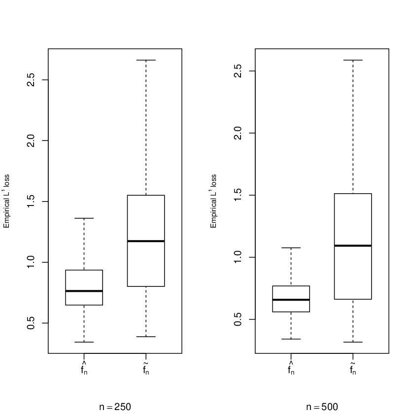
We illustrate the theoretical results by a limited simulation study comparing the performance of f^n\widehat{f}_{n} and the isotonic LSE f~n\widetilde{f}_{n} in terms of their L1L^{1} error. More specifically, consider the following Poisson count time series model, as described in Example 3.1, where we have assumed that ZtZ_{t} is a deterministic trend, i.e. for t=1,2,…,nt=1,2,\ldots,n

Yt∣ℱt−1∼Poisson(λt),λt=f(Yt−1,Zt−1),Y_{t}\mid{\mathcal{F}}_{t-1}\,\sim\,\mbox{Poisson}(\lambda_{t}),~~\lambda_{t}\,=\,f(Y_{t-1},Z_{t-1}),

where

f⁡(y,z)=−5+201+exp⁡(−0.3​y)+4​z and Zt=tn.f(y,z)=-5+\frac{20}{1+\exp(-0.3y)}+4z\qquad\text{ and }\qquad Z_{t}=\frac{t}{n}.

We compute the isotonic least squares estimator by using the R package isotonic.pen which returns the values of the estimated function on an equidistant 21× 2121\,\times\,21 grid; see Wu et al. (2005) for details. Note that f^n=(f¯n+f¯n)/2\widehat{f}_{n}=(\bar{f}_{n}+\underline{f}_{n})/2 can be computed (exactly) on any grid. We use the grid employed by isotonic.pen discarding some points so that we can avoid any boundary issues. To this end, we choose the lower left / upper right corner of the grid such that, on the one hand, the number of observed information variables within the corresponding rectangle is maximized and on the other hand, for every grid point all upper and lower rectangles contain at least one data point. To compare the empirical performance of the estimators, we compute the integrated L1L^{1} error over the grid values. This process is repeated 500 times. Figure 1 shows box plots of the values of integrated L1L^{1} error for two different sample sizes and illustrates that f^n\widehat{f}_{n} achieves smaller error than the isotonic LSE.
Refer to caption
Figure 1. Box plots of empirical L1L^{1} loss values for f^n\widehat{f}_{n} and the isotonic LSE f~n\widetilde{f}_{n}.

4.2. Data Examples

We apply the methodology to biological and financial time series which exhibit some form of non-stationarity. First, we investigate the population growth of whooping cranes that became nearly extinct during the period 1938-1955. Whooping cranes are one of the largest birds in North America but also one of the rarest that can be found in the continent. For some time their population has been constantly decreasing and reached to about 20 individual birds in the world. With the employment of various conservation measures the population grew over the last years. The data we have are depicted in Figure 2 which shows the growth of population of whooping cranes between 1938 to 2005; see Int. Recovery Plan (2007). Note that this is a case of an integer valued time series. The second example refers to daily net asset value (NAV) of the BlackRock Global Allocation Fund during the period 1/4/2016 to 30/1/2018. Here we note that series takes values on real numbers.

For both of these data examples, a simple time series plot reveals increasing trend and strong autocorrelation which decays slowly. The partial autocorrelation functions shows a strong autocorrelation at lag 1; see the upper panel of Figures 2 and 3. We fit a non-parametric time series model to these data by using isotonic estimation methods. We include the covariate vector It=(Yt−1,t/n)′I_{t}=(Y_{t-1},t/n)^{\prime}, where nn is number of effective observations (e.g. for the population growth of whooping cranes the number of observation is equal to 68 but n=67n=67 because of the inclusion of Yt−1Y_{t-1}). We consider again the estimator f^n\widehat{f}_{n} and the isotonic LSE f~n\widetilde{f}_{n} and work the same way as it was explained in Subsection 4.1 . The lower panels of Figures 2 and 3 show that both estimators are quite close near the observation points, but differ significantly at some grid points that are located far from the bulk of data. We examine the performance of both methods for estimating the two models. This task is accomplished by studying the in sample predictive power using the mean absolute prediction error (MAPE), that is ∑t=1n|Y^t−Yt|/n\sum_{t=1}^{n}|\widehat{Y}_{t}-Y_{t}|/n. Here, Y^t\widehat{Y}_{t} is obtained by evaluating f^n\widehat{f}_{n} and f~n\widetilde{f}_{n}, respectively, on a grid point close to (Yt−1,t/n)′(Y_{t-1},t/n)^{\prime}. The results are shown in Table 1. Clearly, the new estimator f^n\widehat{f}_{n} outperforms the isotonic LSE in terms of MAPE for both data examples.

Refer to caption
Figure 2. (a) Time series plot of the yearly number of whooping cranes between 1938 to 2005. (b) Autocorrelation function. (c) Partial autocorrelation function. (d) Plot of isotonic LSE f~n\widetilde{f}_{n} and the data (red points). (e) Plot of the estimator f^n\widehat{f}_{n} and the data (red points). (f) Plot of the difference f~n−f^n\widetilde{f}_{n}-\widehat{f}_{n}.
Refer to caption
Figure 3. (a) Time series plot of daily NAV prices of BlackRock Global Allocation Fund during the period 1/4/2016 to 30/1/2018. (b) Autocorrelation function. (c) Partial autocorrelation function. (d) Plot of isotonic LSE f~n\widetilde{f}_{n} and the data (red points). (e) Plot of the estimator f^n\widehat{f}_{n} and the data (red points). (f) Plot of the difference f~n−f^n\widetilde{f}_{n}-\widehat{f}_{n}.
Example 1 (Whooping cranes) Example 2 (BlackRock Global Allocation Fund)
f^n\widehat{f}_{n} 5.916453 0.3108097
f~n\widetilde{f}_{n} 6.002488 0.3118416
Table 1. MAPE obtained from our estimator f^n\widehat{f}_{n} and the isotonic LSE f~n\widetilde{f}_{n}.

5. Proofs and Auxiliary Results

We prove our main results in Section 5.1. Some auxiliary lemmas are stated and proved in Section 5.2.

5.1. Proofs of the main results

Proof of Lemma 2.1.

Since ∑t=1nP⁡(It∈Bk)≥n​C1​hnd≥C1​n2/(d+2)\sum_{t=1}^{n}P(I_{t}\in B_{k})\geq nC_{1}h_{n}^{d}\geq C_{1}n^{2/(d+2)} it suffices to show that

∑k∈KnP(∑t=1nP(It∈Bk)− 1(It∈Bk)≥C1​n2/(d+2)2)⟶n→∞ 0,\sum_{k\in K_{n}}P\left(\sum_{t=1}^{n}P(I_{t}\in B_{k})\,-\,{\mathbbm{1}}(I_{t}\in B_{k})\,\geq\,\frac{C_{1}\;n^{2/(d+2)}}{2}\right)\,\mathop{\longrightarrow}\limits_{n\to\infty}\,0, (5.1)

by recalling that 𝟙(.){\mathbbm{1}}(.) denotes the indicator function. We obtain from Bernstein’s inequality, for all k∈Knk\in K_{n} and μn=C1​n2/(d+2)/2\mu_{n}=C_{1}n^{2/(d+2)}/2, that

P⁡(∑t=1nP⁡(It∈Bk)− 1​(It∈Bk)≥μn)\displaystyle P\left(\sum_{t=1}^{n}P(I_{t}\in B_{k})\,-\,{\mathbbm{1}}(I_{t}\in B_{k})\,\geq\,\mu_{n}\right) ≤\displaystyle\leq exp⁡{−μn2/2n​P​(I1∈Bk)​(1−P⁡(I1∈Bk))+μn/3}\displaystyle\exp\left\{-\;\frac{\mu_{n}^{2}/2}{n\;P(I_{1}\in B_{k})\;(1-P(I_{1}\in B_{k}))\,+\,\mu_{n}/3}\right\}
≤\displaystyle\leq exp⁡{−C​n2/(d+2)},\displaystyle\exp\left\{-\;C\;n^{2/(d+2)}\right\},

for some C>0C>0, which proves (5.1). ∎

Proof of Theorem 2.1.

We analyze the contribution of the stochastic part and the bias of the estimator separately. For the latter, we exploit the assumed isotonicity in conjunction with boundedness of ff in order to construct an estimate of the integrated bias from above and below. To this end, denote for an arbitrary function gg its positive (respectively negative) part by g+g_{+} (respectively g−g_{-}). Then, it suffices to show that

E⁡[∫Dn(f^n​(x)−f⁡(x))+​λd​(𝑑x)​  1An]\displaystyle E\left[\int_{D_{n}}\left(\widehat{f}_{n}(x)\,-\,f(x)\right)_{+}\,\lambda^{d}(dx)\;\;{\mathbbm{1}}_{A_{n}}\right] =O(n−1/(d+2)),\displaystyle=O\left(n^{-1/(d+2)}\right), (5.2a)
and
E⁡[∫Dn(f^n​(x)−f⁡(x))−​λd​(𝑑x)​  1An]\displaystyle E\left[\int_{D_{n}}\left(\widehat{f}_{n}(x)\,-\,f(x)\right)_{-}\,\lambda^{d}(dx)\;\;{\mathbbm{1}}_{A_{n}}\right] =O(n−1/(d+2)).\displaystyle=O\left(n^{-1/(d+2)}\right). (5.2b)

We have, for all x∈Bk=(xk−𝟏,xk]x\in B_{k}=\bm{(}x_{k-\mathbf{1}},x_{k}\bm{]},

(f^n​(x)−f⁡(x))+\displaystyle\left(\widehat{f}_{n}(x)\,-\,f(x)\right)_{+} ≤\displaystyle\leq (supy⪯xkAvY​((y,xk+𝟏])−f⁡(x))+\displaystyle\left(\sup_{y\preceq x_{k}}\mbox{Av}_{Y}(\bm{(}y,x_{k+\mathbf{1}}\bm{]})\,-\,f(x)\right)_{+} (5.3)
≤\displaystyle\leq supy⪯xk|Avε​((y,xk+𝟏])|+(f⁡(xk+𝟏)−f⁡(x)).\displaystyle\sup_{y\preceq x_{k}}\left|\mbox{Av}_{\varepsilon}(\bm{(}y,x_{k+\mathbf{1}}\bm{]})\right|\,+\,\left(f(x_{k+\mathbf{1}})\,-\,f(x)\right).

By Lemma 5.1 and since λd(Bk)=hnd=O(n−d/(d+2))\lambda^{d}(B_{k})=h_{n}^{d}=O(n^{-d/(d+2)}) we obtain for the bias that

∑k: 1<k1,…,kd<Mn∫Bk(f(xk+𝟏)−f(x))λd(dx)\displaystyle\sum_{k\colon\,1<k_{1},\ldots,k_{d}<M_{n}}\int_{B_{k}}\left(f(x_{k+\mathbf{1}})\,-\,f(x)\right)\,\lambda^{d}(dx) (5.4)
≤\displaystyle\leq ∑k: 1<k1,…,kd<Mn(f(xk+𝟏)−f(xk−𝟏))λd(Bk)=O(n−1/(d+2)).\displaystyle\sum_{k\colon\,1<k_{1},\ldots,k_{d}<M_{n}}\left(f(x_{k+\mathbf{1}})\,-\,f(x_{k-\mathbf{1}})\right)\;\lambda^{d}(B_{k})\,=\,O\left(n^{-1/(d+2)}\right).

For the stochastic part, we estimate E⁡[supy⪯xk|Avε​((y,xk+𝟏])|]\;E[\sup_{y\preceq x_{k}}|\mbox{Av}_{\varepsilon}(\bm{(}y,x_{k+\mathbf{1}}\bm{]})|]. For this purpose, we define a dyadic scheme of nested hyperrectangles: For j1,…,jd≥0j_{1},\ldots,j_{d}\geq 0,

Bk(j1,…,jd)=((k1+1−2j1)hn,(k1+1)hn]×⋯×((kd+1−2jd)hn,(kd+1)hn].B_{k}^{(j_{1},\ldots,j_{d})}\,=\,((k_{1}+1-2^{j_{1}})h_{n},(k_{1}+1)h_{n}]\times\cdots\times((k_{d}+1-2^{j_{d}})h_{n},(k_{d}+1)h_{n}].

(We have in particular Bk(0,…,0)=Bk+𝟏B_{k}^{(0,\ldots,0)}=B_{k+\mathbf{1}} and Bk(j1,…,jd)=⋃m1,…,md: 0≤mi≤2ji−1B(k1+1−m1,…,kd+1−md)B_{k}^{(j_{1},\ldots,j_{d})}=\bigcup_{m_{1},\ldots,m_{d}\colon\,0\leq m_{i}\leq 2^{j_{i}}-1}B_{(k_{1}+1-m_{1},\ldots,k_{d}+1-m_{d})}.) Since {y⪯xk}⊆⋃j1,…,jd≥0Bk(j1+1,…,jd+1)∖Bk(j1,…,jd)\{y\preceq x_{k}\}\subseteq\bigcup_{j_{1},\ldots,j_{d}\geq 0}B_{k}^{(j_{1}+1,\ldots,j_{d}+1)}\setminus B_{k}^{(j_{1},\ldots,j_{d})} and since y∈Bk(j1+1,…,jd+1)∖Bk(j1,…,jd)y\in B_{k}^{(j_{1}+1,\ldots,j_{d}+1)}\setminus B_{k}^{(j_{1},\ldots,j_{d})} implies that (y,xk+𝟏]⊇Bk(j1,…,jd)\bm{(}y,x_{k+\mathbf{1}}\bm{]}\supseteq B_{k}^{(j_{1},\ldots,j_{d})} we obtain, for all x∈Bkx\in B_{k},

supy⪯xk|Avε((y,xk+𝟏])|≤∑j1,…,jd≥0sup{|∑t=1nεt​𝟙​(It∈(y,xk+𝟏])|:y∈Bk(j1+1,…,jd+1)∖Bk(j1,…,jd)}#⁡{t≤n:It∈Bk(j1,…,jd)}.\sup_{y\preceq x_{k}}\left|\mbox{Av}_{\varepsilon}(\bm{(}y,x_{k+\mathbf{1}}\bm{]})\right|\,\leq\,\sum_{j_{1},\ldots,j_{d}\geq 0}\frac{\sup\left\{\left|\sum_{t=1}^{n}\varepsilon_{t}{\mathbbm{1}}(I_{t}\in\bm{(}y,x_{k+\mathbf{1}}\bm{]})\right|\colon\;\;y\in B_{k}^{(j_{1}+1,\ldots,j_{d}+1)}\setminus B_{k}^{(j_{1},\ldots,j_{d})}\right\}}{\#\left\{t\leq n\colon\;\;I_{t}\in B_{k}^{(j_{1},\ldots,j_{d})}\right\}}.

Recall that if the event AnA_{n} occurs, then #⁡{t≤n:It∈Bk}≥(C1/2)​n2/(d+2)\#\{t\leq n\colon\;I_{t}\in B_{k}\}\geq(C_{1}/2)\,n^{2/(d+2)} for all k∈Knk\in K_{n}, which implies that

#⁡{t≤n:It∈Bk(j1,…,jd)}≥(C1/2)​ 2j1+⋯+jd​n2/(d+2).\#\left\{t\leq n\colon\;\;I_{t}\in B_{k}^{(j_{1},\ldots,j_{d})}\right\}\,\geq\,(C_{1}/2)\;2^{j_{1}+\cdots+j_{d}}\;n^{2/(d+2)}.

Furthermore, it follows from Lemma 5.2 that for some C<∞C<\infty

E⁡[sup{|∑t=1nεt​𝟙​(It∈(y,xk+𝟏])|:y∈Bk(j1+1,…,jd+1)}]≤C​ 2(j1+⋯+jd)/2​n1/(d+2).E\left[\sup\left\{\left|\sum_{t=1}^{n}\varepsilon_{t}{\mathbbm{1}}(I_{t}\in\bm{(}y,x_{k+\mathbf{1}}\bm{]})\right|\colon\;\;y\in B_{k}^{(j_{1}+1,\ldots,j_{d}+1)}\right\}\right]\,\leq\,C\;2^{(j_{1}+\cdots+j_{d})/2}\;n^{1/(d+2)}. (5.5)

Therefore, we obtain that

supx∈BkE⁡[supy⪯xk|Avε​((y,xk+𝟏])|​  1An]\displaystyle\sup_{x\in B_{k}}E\left[\sup_{y\preceq x_{k}}\left|\mbox{Av}_{\varepsilon}(\bm{(}y,x_{k+\mathbf{1}}\bm{]})\right|\;\;{\mathbbm{1}}_{A_{n}}\right]
≤\displaystyle\leq ∑j1,…,jd≥0E[sup{|∑t=1nεt 1(It∈(y,xk+𝟏])|:y∈Bk(j1+1,…,jd+1)}#⁡{t≤n:It∈Bk(j1,…,jd)}  1An]\displaystyle\sum_{j_{1},\ldots,j_{d}\geq 0}E\left[\frac{\sup\left\{\left|\sum_{t=1}^{n}\varepsilon_{t}\;{\mathbbm{1}}(I_{t}\in\bm{(}y,x_{k+\mathbf{1}}\bm{]})\right|\colon\quad y\in B_{k}^{(j_{1}+1,\ldots,j_{d}+1)}\right\}}{\#\{t\leq n\colon\;I_{t}\in B_{k}^{(j_{1},\ldots,j_{d})}\}}\;\;{\mathbbm{1}}_{A_{n}}\right]
=\displaystyle= O(n−1/(d+2)∑j1,…,jd≥02−(j1+⋯+jd)/2)=O(n−1/(d+2)).\displaystyle O\left(n^{-1/(d+2)}\;\sum_{j_{1},\ldots,j_{d}\geq 0}2^{-(j_{1}+\cdots+j_{d})/2}\right)\,=\,O\left(n^{-1/(d+2)}\right).

This yields, in conjunction with (5.3) and (5.4), that (5.2a) holds. The proof of (5.2b) is completely analogous and therefore it is omitted. ∎

Proof of Lemma 3.1.

Analogously to the proof of Lemma 2.1, we will show that

maxk∈K~n{P(∑t=1nP(It∈B~k)− 1(It∈B~k)≥C1​n2/(d2+2)2)}=o(n−d2/(d2+2)).\max_{k\in\widetilde{K}_{n}}\left\{P\left(\sum_{t=1}^{n}P(I_{t}\in\widetilde{B}_{k})\,-\,{\mathbbm{1}}(I_{t}\in\widetilde{B}_{k})\,\geq\,\frac{C_{1}\;n^{2/(d_{2}+2)}}{2}\right)\right\}\,=\,o\left(n^{-d_{2}/(d_{2}+2)}\right). (5.6)

Let μn=C1​n2/(d2+2)/8\mu_{n}={C_{1}n^{2/(d_{2}+2)}}/{8} and, for arbitrary k∈K~nk\in\widetilde{K}_{n}, ηt=𝟙​(It∈B~k)−P⁡(It∈B~k)\eta_{t}={\mathbbm{1}}(I_{t}\in\widetilde{B}_{k})-P(I_{t}\in\widetilde{B}_{k}). It follows from the Fuk-Nagaev-type inequality (I.6) of Rio (2000, page 4) that, for all κ≥1\kappa\geq 1,

P(|∑t=1nηt|≥ 4μn)≤((1+μn2κ​sn2)−κ/2+n​α​([μn/κ])μn),P\left(\left|\sum_{t=1}^{n}\eta_{t}\right|\,\geq\,4\,\mu_{n}\right)\,\leq\,\;\left(\left(1\,+\,\frac{\mu_{n}^{2}}{\kappa\;s_{n}^{2}}\right)^{-\kappa/2}\,+\,\frac{n\;\alpha([\mu_{n}/\kappa])}{\mu_{n}}\right), (5.7)

where

sn2=∑s,t=1n|cov(ηs,ηt)|.s_{n}^{2}\,=\,\sum_{s,t=1}^{n}\left|\mathop{\rm cov}\nolimits(\eta_{s},\eta_{t})\right|.

Note that (A2)(ii) implies that

α⁡(N)=o⁡(N−d2)and∑r=N∞α⁡(r)=o⁡(N1−d2).\alpha(N)=o(N^{-d_{2}})\qquad\text{and}\qquad\sum_{r=N}^{\infty}\alpha(r)=o(N^{1-d_{2}}). (5.8)

To see the first relationship of (5.8), note that, for j∈ℕj\in{\mathbb{N}},

α⁡(2j)\displaystyle\alpha(2^{j}) ≤\displaystyle\leq 12j−1​∑r=2j−1+12jα⁡(r)≤12j−1​∑r=2j−1+12j(r2j−1)d2−1​α​(r)\displaystyle\frac{1}{2^{j-1}}\sum_{r=2^{j-1}+1}^{2^{j}}\alpha(r)\leq\frac{1}{2^{j-1}}\sum_{r=2^{j-1}+1}^{2^{j}}\left(\frac{r}{2^{j-1}}\right)^{d_{2}-1}\alpha(r)
=\displaystyle= 2(1−j)​d2​∑r=2j−1+12jrd2−1​α​(r),\displaystyle 2^{(1-j)d_{2}}\sum_{r=2^{j-1}+1}^{2^{j}}r^{d_{2}-1}\alpha(r),

which implies that 2d2​jα(2j)⟶j→∞02^{d_{2}j}\alpha(2^{j})\mathop{\longrightarrow}_{j\to\infty}0. Since the sequence (α⁡(r))r∈ℕ(\alpha(r))_{r\in{\mathbb{N}}} is monotonically non-increasing, we obtain that α⁡(N)=o⁡(N−d2)\alpha(N)=o(N^{-d_{2}}). Note that the second relationship of (5.8) follows from Nd2−1∑r=N∞α(r)≤∑r=N∞rd2−1α(r)⟶j→∞0N^{d_{2}-1}\sum_{r=N}^{\infty}\alpha(r)\,\leq\,\sum_{r=N}^{\infty}r^{d_{2}-1}\alpha(r)\mathop{\longrightarrow}_{j\to\infty}0.

Since α([μn/κ])=o(n−2d2/(d2+2))\alpha([\mu_{n}/\kappa])=o(n^{-2d_{2}/(d_{2}+2)}) we obtain that

n​α​([μn/κ])μn=o(nn−2d2/(d2+2)n−2/(d2+2))=o(n−d2/(d2+2)),\frac{n\;\alpha([\mu_{n}/\kappa])}{\mu_{n}}\,=\,o\left(n\;n^{-2d_{2}/(d_{2}+2)}\;n^{-2/(d_{2}+2)}\right)\,=\,o\left(n^{-d_{2}/(d_{2}+2)}\right),

that is, the second term on the right-hand side of (5.7) is of the required order. It remains to estimate sn2s_{n}^{2}. To this end, we distinguish between the two cases of covariates without and with a trend component. In the first case, we obtain from the upper bound in (A3)(i) that, for all t,rt,r with 1≤t≤t+r≤n1\leq t\leq t+r\leq n,

|cov(ηt,ηt+r)|={O(n−d2/(d2+2)) if ​0≤r<d,O(n−2d2/(d2+2)) if ​r≥d.\displaystyle\left|\mathop{\rm cov}\nolimits(\eta_{t},\eta_{t+r})\right|\,=\,\left\{\begin{array}[]{ll}O\left(n^{-d_{2}/(d_{2}+2)}\right)&\quad\mbox{ if }0\leq r<d,\\ O\left(n^{-2d_{2}/(d_{2}+2)}\right)&\quad\mbox{ if }r\geq d\end{array}\right..

On the other hand, we obtain from a covariance inequality for strong mixing processes (see e.g. Bradley (2007, Corollary 10.16)) that

|cov(ηt,ηt+r)|≤ 4​α​(r)​‖ηt‖∞​‖ηt+r‖∞≤ 4​α​(r).\left|\mathop{\rm cov}\nolimits(\eta_{t},\eta_{t+r})\right|\,\leq\,4\;\alpha(r)\;\|\eta_{t}\|_{\infty}\;\|\eta_{t+r}\|_{\infty}\,\leq\,4\;\alpha(r).

Therefore, with Nn=[nd2/(d2+2)]N_{n}=[n^{d_{2}/(d_{2}+2)}],

sn2\displaystyle s_{n}^{2} ≤\displaystyle\leq ∑s,t:|s−t|<d|cov(ηs,ηt)|+∑s,t:d≤|s−t|≤Nn|cov(ηs,ηt)|+ 2n∑r=Nn+1n−14α(r)\displaystyle\sum_{s,t\colon\;|s-t|<d}\left|\mathop{\rm cov}\nolimits(\eta_{s},\eta_{t})\right|\,+\,\sum_{s,t\colon\;d\leq|s-t|\leq N_{n}}\left|\mathop{\rm cov}\nolimits(\eta_{s},\eta_{t})\right|\,+\,2n\;\sum_{r=N_{n}+1}^{n-1}4\;\alpha(r) (5.10)
=\displaystyle= O⁡(n2/(d2+2))+O⁡(n2/(d2+2))+o⁡(n​Nn1−d2)\displaystyle O\left(n^{2/(d_{2}+2)}\right)\,+\,O\left(n^{2/(d_{2}+2)}\right)\,+\,o\left(n\;N_{n}^{1-d_{2}}\right)
=\displaystyle= O⁡(n2/(d2+2))+o⁡(n2/(d2+2)​n(2−d2)​d2/(d2+2)).\displaystyle O\left(n^{2/(d_{2}+2)}\right)\,+\,o\left(n^{2/(d_{2}+2)}\;n^{(2-d_{2})d_{2}/(d_{2}+2)}\right).

In the case with trend, we get from (A3)(i) that

|cov(ηt,ηt+r)|={O(n−(d2−1)/(d2+2)) if ​0≤r<d−1,O(n−2(d2−1)/(d2+2)) if ​r≥d−1.\displaystyle\left|\mathop{\rm cov}\nolimits(\eta_{t},\eta_{t+r})\right|\,=\,\left\{\begin{array}[]{ll}O\left(n^{-(d_{2}-1)/(d_{2}+2)}\right)&\quad\mbox{ if }0\leq r<d-1,\\ O\left(n^{-2(d_{2}-1)/(d_{2}+2)}\right)&\quad\mbox{ if }r\geq d-1\end{array}\right..

On the other hand, we see that It=(I~t′,t/n)′∉B~kI_{t}=(\widetilde{I}_{t}^{\prime},t/n)^{\prime}\not\in\widetilde{B}_{k}, and therefore ηt=0\eta_{t}=0 if t∉In,k:=((kd−1)​n​hn,kd​n​hn]t\not\in I_{n,k}:=((k_{d}-1)nh_{n},k_{d}nh_{n}]. Hence, here with Nn=[n(d2−1)/(d2+2)]N_{n}=[n^{(d_{2}-1)/(d_{2}+2)}],

sn2\displaystyle s_{n}^{2} ≤\displaystyle\leq ∑s,t∈In,k|cov(ηs,ηt)|\displaystyle\sum_{s,t\in I_{n,k}}\left|\mathop{\rm cov}\nolimits(\eta_{s},\eta_{t})\right| (5.12)
=\displaystyle= O(∑(s,t)∈In,k:|s−t|<d−1|cov(ηs,ηt)|+∑(s,t)∈In,k:d−1≤|s−t|≤Nn|cov(ηs,ηt)|+nhn∑r=Nn+1n−14α(r))\displaystyle O\left(\sum_{(s,t)\in I_{n,k}\colon\;|s-t|<d-1}\left|\mathop{\rm cov}\nolimits(\eta_{s},\eta_{t})\right|\,+\,\sum_{(s,t)\in I_{n,k}\colon\;d-1\leq|s-t|\leq N_{n}}\left|\mathop{\rm cov}\nolimits(\eta_{s},\eta_{t})\right|\,+\,nh_{n}\;\sum_{r=N_{n}+1}^{n-1}4\;\alpha(r)\right)
=\displaystyle= O⁡(n2/(d2+2))+o⁡(n2/(d2+2)​n(2−d2)​(d2−1)/(d2+2)).\displaystyle O\left(n^{2/(d_{2}+2)}\right)\,+\,o\left(n^{2/(d_{2}+2)}\;n^{(2-d_{2})(d_{2}-1)/(d_{2}+2)}\right).

We see from (5.10) and (5.12) that in the two cases without and with trend the term (1+μn2/(κ​sn2))−1(1+\mu_{n}^{2}/(\kappa s_{n}^{2}))^{-1} is of order O⁡(n−γ)O(n^{-\gamma}), for some γ>0\gamma>0. Choosing κ>2​d2/γ\kappa>2d_{2}/\gamma we see that (5.6) follows from (5.7), which completes the proof. ∎

Proof of Theorem 3.1.

The proof of this theorem is largely the same as that of Theorem 2.1. We show that

E[∫D~n(f^n(x)−f(x))+ν(dx)  1A~n]=O(n−1/(d2+2)),E\left[\int_{\widetilde{D}_{n}}\left(\widehat{f}_{n}(x)\,-\,f(x)\right)_{+}\,\nu(dx)\;\;{\mathbbm{1}}_{\widetilde{A}_{n}}\right]\,=\,O\left(n^{-1/(d_{2}+2)}\right), (5.13a)
and
E[∫D~n(f^n(x)−f(x))−ν(dx)  1A~n]=O(n−1/(d2+2)).E\left[\int_{\widetilde{D}_{n}}\left(\widehat{f}_{n}(x)\,-\,f(x)\right)_{-}\,\nu(dx)\;\;{\mathbbm{1}}_{\widetilde{A}_{n}}\right]\,=\,O\left(n^{-1/(d_{2}+2)}\right). (5.13b)

We define grid points

xk\displaystyle x_{k} =\displaystyle= (k1,…,kd1,G1−1​(kd1+1​hn),…,Gd2−1​(kd​hn))′,\displaystyle\left(k_{1},\ldots,k_{d_{1}},G_{1}^{-1}(k_{d_{1}+1}h_{n}),\ldots,G_{d_{2}}^{-1}(k_{d}h_{n})\right)^{\prime},
x¯k\displaystyle\overline{x}_{k} =\displaystyle= (k1,…,kd1,G1−1​((kd1+1+1)​hn),…,Gd2−1​((kd+1)​hn))′,\displaystyle\left(k_{1},\ldots,k_{d_{1}},G_{1}^{-1}((k_{d_{1}+1}+1)h_{n}),\ldots,G_{d_{2}}^{-1}((k_{d}+1)h_{n})\right)^{\prime},
x¯k\displaystyle\underline{x}_{k} =\displaystyle= (k1,…,kd1,G1−1​((kd1+1−1)​hn),…,Gd2−1​((kd−1)​hn))′.\displaystyle\left(k_{1},\ldots,k_{d_{1}},G_{1}^{-1}((k_{d_{1}+1}-1)h_{n}),\ldots,G_{d_{2}}^{-1}((k_{d}-1)h_{n})\right)^{\prime}.

We have, for all x∈B~k=(x¯k,xk]x\in\widetilde{B}_{k}=\bm{(}\underline{x}_{k},x_{k}\bm{]},

(f^n​(x)−f⁡(x))+\displaystyle\left(\widehat{f}_{n}(x)\,-\,f(x)\right)_{+} ≤\displaystyle\leq (supy⪯xkAvY​((y,x¯k])−f⁡(x))+\displaystyle\left(\sup_{y\preceq x_{k}}\mbox{Av}_{Y}(\bm{(}y,\overline{x}_{k}\bm{]})\,-\,f(x)\right)_{+} (5.14)
≤\displaystyle\leq supy⪯xk|Avε​((y,x¯k])|+(f⁡(x¯k)−f⁡(x)).\displaystyle\sup_{y\preceq x_{k}}\left|\mbox{Av}_{\varepsilon}(\bm{(}y,\overline{x}_{k}\bm{]})\right|\,+\,\left(f(\overline{x}_{k})\,-\,f(x)\right).

We apply Lemma 5.1 to f~​(x~1,…,x~d2)=f⁡(k1,…,kd1,G1−1​(x~1),…,Gd2−1​(x~d2))\widetilde{f}(\widetilde{x}_{1},\dots,\widetilde{x}_{d_{2}})=f(k_{1},\ldots,k_{d_{1}},G_{1}^{-1}(\widetilde{x}_{1}),\ldots,G_{d_{2}}^{-1}(\widetilde{x}_{d_{2}})), (x~1,…,x~d2)′∈[0,1]d2,(\widetilde{x}_{1},\dots,\widetilde{x}_{d_{2}})^{\prime}\in[0,1]^{d_{2}}, with M=M~nM=\widetilde{M}_{n}. Since νd(B~k)=h~nd2=O(n−d2/(d2+2))\nu^{d}(\widetilde{B}_{k})=\widetilde{h}_{n}^{d_{2}}=O(n^{-d_{2}/(d_{2}+2)}) we obtain for the bias that

∑k: 1<kd1+1,…,kd<M~n∫B~k(f(x¯k)−f(x))ν(dx)\displaystyle\sum_{k\colon\,1<k_{d_{1}+1},\ldots,k_{d}<\widetilde{M}_{n}}\int_{\widetilde{B}_{k}}\left(f(\overline{x}_{k})\,-\,f(x)\right)\,\nu(dx) (5.15)
≤\displaystyle\leq ∑k: 1<kd1+1,…,kd<M~n(f(x¯k)−f(x¯k))ν(B~k)=O(M~nd2−1h~nd2)=O(n−1/(d2+2)).\displaystyle\sum_{k\colon\,1<k_{d_{1}+1},\ldots,k_{d}<\widetilde{M}_{n}}\left(f(\overline{x}_{k})\,-\,f(\underline{x}_{k})\right)\;\nu(\widetilde{B}_{k})\,=\,O\left(\widetilde{M}_{n}^{d_{2}-1}\;\widetilde{h}_{n}^{d_{2}}\right)\,=\,O\left(n^{-1/(d_{2}+2)}\right).\qquad

We define again a dyadic scheme of nested hyperrectangles: For j1,…,jd2≥0j_{1},\ldots,j_{d_{2}}\geq 0,

B~k(j1,…,jd2)={(k1,…,kd1)′}×((kd1+1+1−2j1)h~n,(kd1+1+1)h~n]×⋯×((kd+1−2jd2)h~n,(kd+1)h~n]\widetilde{B}_{k}^{(j_{1},\ldots,j_{d_{2}})}\,=\,\{(k_{1},\ldots,k_{d_{1}})^{\prime}\}\times((k_{d_{1}+1}+1-2^{j_{1}})\widetilde{h}_{n},(k_{d_{1}+1}+1)\widetilde{h}_{n}]\times\cdots\times((k_{d}+1-2^{j_{d_{2}}})\widetilde{h}_{n},(k_{d}+1)\widetilde{h}_{n}]

and

B~k,0(j1,…,jd2)={0,…,k1}×⋯×{0,…,kd1}×((kd1+1+1−2j1)h~n,(kd1+1+1)h~n]×⋯×((kd+1−2jd2)h~n,(kd+1)h~n].\widetilde{B}_{k,0}^{(j_{1},\ldots,j_{d_{2}})}\,=\,\{0,\ldots,k_{1}\}\times\cdots\times\{0,\ldots,k_{d_{1}}\}\times((k_{d_{1}+1}+1-2^{j_{1}})\widetilde{h}_{n},(k_{d_{1}+1}+1)\widetilde{h}_{n}]\times\cdots\times((k_{d}+1-2^{j_{d_{2}}})\widetilde{h}_{n},(k_{d}+1)\widetilde{h}_{n}].

Since {y⪯xk}⊆⋃j1,…,jd2≥0B~k,0(j1+1,…,jd2+1)∖B~k,0(j1,…,jd2)\{y\preceq x_{k}\}\subseteq\bigcup_{j_{1},\ldots,j_{d_{2}}\geq 0}\widetilde{B}_{k,0}^{(j_{1}+1,\ldots,j_{d_{2}}+1)}\setminus\widetilde{B}_{k,0}^{(j_{1},\ldots,j_{d_{2}})} and since y∈B~k,0(j1+1,…,jd2+1)∖B~k,0(j1,…,jd2)y\in\widetilde{B}_{k,0}^{(j_{1}+1,\ldots,j_{d_{2}}+1)}\setminus\widetilde{B}_{k,0}^{(j_{1},\ldots,j_{d_{2}})} implies that (y,x¯k]⪰B~k(j1,…,jd2)\bm{(}y,\overline{x}_{k}\bm{]}\succeq\widetilde{B}_{k}^{(j_{1},\ldots,j_{d_{2}})} we obtain, for all x∈B~kx\in\widetilde{B}_{k},

supy⪯xk|Avε((y,x¯k])|≤∑j1,…,jd2≥0sup{|∑t=1nεt​𝟙​(It∈(y,x¯k])|:y∈B~k,0(j1+1,…,jd2+1)∖B~k,0(j1,…,jd2)}#⁡{t≤n:It∈B~k(j1,…,jd2)}.\sup_{y\preceq x_{k}}\left|\mbox{Av}_{\varepsilon}(\bm{(}y,\overline{x}_{k}\bm{]})\right|\,\leq\,\sum_{j_{1},\ldots,j_{d_{2}}\geq 0}\frac{\sup\left\{\left|\sum_{t=1}^{n}\varepsilon_{t}{\mathbbm{1}}(I_{t}\in\bm{(}y,\overline{x}_{k}\bm{]})\right|\colon\;\;y\in\widetilde{B}_{k,0}^{(j_{1}+1,\ldots,j_{d_{2}}+1)}\setminus\widetilde{B}_{k,0}^{(j_{1},\ldots,j_{d_{2}})}\right\}}{\#\left\{t\leq n\colon\;\;I_{t}\in\widetilde{B}_{k}^{(j_{1},\ldots,j_{d_{2}})}\right\}}.

Recall that if the event A~n\widetilde{A}_{n} occurs, then #⁡{t≤n:It∈B~k}≥(C1/2)​n2/(d2+2)\#\{t\leq n\colon\;I_{t}\in\widetilde{B}_{k}\}\geq(C_{1}/2)\,n^{2/(d_{2}+2)} for all k∈K~nk\in\widetilde{K}_{n}, which implies that

#⁡{t≤n:It∈B~k(j1,…,jd2)}≥(C1/2)​ 2j1+⋯+jd2​n2/(d2+2).\#\left\{t\leq n\colon\;\;I_{t}\in\widetilde{B}_{k}^{(j_{1},\ldots,j_{d_{2}})}\right\}\,\geq\,(C_{1}/2)\;2^{j_{1}+\cdots+j_{d_{2}}}\;n^{2/(d_{2}+2)}.

Furthermore, it follows from Lemma 5.3 that for some C<∞C<\infty

E⁡[sup{|∑t=1nεt​𝟙​(It∈(y,x¯k])|:y∈B~k,0(j1+1,…,jd2+1)}]≤C​ 2(j1+⋯+jd2)/2​n1/(d2+2).E\left[\sup\left\{\left|\sum_{t=1}^{n}\varepsilon_{t}{\mathbbm{1}}(I_{t}\in\bm{(}y,\overline{x}_{k}\bm{]})\right|\colon\;\;y\in\widetilde{B}_{k,0}^{(j_{1}+1,\ldots,j_{d_{2}}+1)}\right\}\right]\,\leq\,C\;2^{(j_{1}+\cdots+j_{d_{2}})/2}\;n^{1/(d_{2}+2)}. (5.16)

Therefore, we obtain that

supx∈B~kE⁡[supy⪯xk|Avε​((y,x¯k])|​  1A~n]\displaystyle\sup_{x\in\widetilde{B}_{k}}E\left[\sup_{y\preceq x_{k}}\left|\mbox{Av}_{\varepsilon}(\bm{(}y,\overline{x}_{k}\bm{]})\right|\;\;{\mathbbm{1}}_{\widetilde{A}_{n}}\right]
≤\displaystyle\leq ∑j1,…,jd2≥0E[sup{|∑t=1nεt 1(It∈(y,x¯k])|:y∈B~k,0(j1+1,…,jd2+1)}#⁡{t≤n:It∈B~k(j1,…,jd2)}  1A~n]\displaystyle\sum_{j_{1},\ldots,j_{d_{2}}\geq 0}E\left[\frac{\sup\left\{\left|\sum_{t=1}^{n}\varepsilon_{t}\;{\mathbbm{1}}(I_{t}\in\bm{(}y,\overline{x}_{k}\bm{]})\right|\colon\quad y\in\widetilde{B}_{k,0}^{(j_{1}+1,\ldots,j_{d_{2}}+1)}\right\}}{\#\{t\leq n\colon\;I_{t}\in\widetilde{B}_{k}^{(j_{1},\ldots,j_{d_{2}})}\}}\;\;{\mathbbm{1}}_{\widetilde{A}_{n}}\right]
=\displaystyle= O(n−1/(d2+2)∑j1,…,jd2≥02−(j1+⋯+jd2)/2)=O(n−1/(d2+2)).\displaystyle O\left(n^{-1/(d_{2}+2)}\;\sum_{j_{1},\ldots,j_{d_{2}}\geq 0}2^{-(j_{1}+\cdots+j_{d_{2}})/2}\right)\,=\,O\left(n^{-1/(d_{2}+2)}\right).

This yields, in conjunction with (5.14) and (5.15), that (5.13a) holds. The proof of (5.13b) is completely analogous and therefore it is omitted. ∎

5.2. Some auxiliary results

Lemma 5.1.

Suppose that f:[0,1]d→ℝf\colon\;[0,1]^{d}\rightarrow{\mathbb{R}} is isotonic and let, for M∈ℕM\in{\mathbb{N}} and k=(k1,…,kd)k=(k_{1},\ldots,k_{d}), xk=(k1/M,…,kd/M)x_{k}=(k_{1}/M,\ldots,k_{d}/M). Then

∑k: 0<k1,…,kd<M(f(xk+𝟏)−f(xk−𝟏))≤ 2dMd−1(f(1,…,1)−f(0,…,0)).\sum_{k\colon\,0<k_{1},\ldots,k_{d}<M}\left(f(x_{k+\bm{1}})\,-\,f(x_{k-\bm{1}})\right)\,\leq\,2d\;M^{d-1}\;\left(f(1,\ldots,1)\,-\,f(0,\ldots,0)\right).
Proof of Lemma 5.1.

Let ℐ0={k: 0<k1,…,kd<M and kj=1 for at least one j}{\mathcal{I}}_{0}=\{k\colon\;0<k_{1},\ldots,k_{d}<M\mbox{ and }k_{j}=1\mbox{ for at least one }j\}. We estimate the sum by considering the main and minor diagonals as follows:

∑k: 0<k1,…,kd<M(f(xk+𝟏)−f(xk−𝟏))\displaystyle\sum_{k\colon\;0<k_{1},\ldots,k_{d}<M}\left(f(x_{k+\mathbf{1}})\,-\,f(x_{k-\mathbf{1}})\right) =\displaystyle= ∑k∈ℐ0∑i≥0(f⁡(xk+(i+1)​𝟏)−f⁡(xk+(i−1)​𝟏))\displaystyle\sum_{k\in{\mathcal{I}}_{0}}\sum_{i\geq 0}\left(f(x_{k+(i+1)\mathbf{1}})\,-\,f(x_{k+(i-1)\mathbf{1}})\right)
≤\displaystyle\leq #​ℐ0​  2​(supx{f⁡(x)}−infx{f⁡(x)}).\displaystyle\#{\mathcal{I}}_{0}\;\;2\left(\sup_{x}\{f(x)\}\,-\,\inf_{x}\{f(x)\}\right).

The assertion of the lemma follows because #​ℐ0≤d​Md−1\#{\mathcal{I}}_{0}\leq dM^{d-1}. ∎

Lemma 5.2.

Suppose that the assumptions of Theorem 2.1 hold true. Then, for arbitrary z¯⪯z¯\underline{z}\preceq\overline{z} with [z¯,z¯]⊆[0,1]d\bm{[}\underline{z},\overline{z}\bm{]}\subseteq[0,1]^{d} and some C¯<∞\bar{C}<\infty,

E[supz:z¯⪯z⪯z¯|1n∑t=1nεt𝟙(It∈(z,z¯])|]≤C¯P⁡(I1∈(z¯,z¯])E\left[\sup_{z\colon\;\underline{z}\preceq z\preceq\overline{z}}\left|\frac{1}{\sqrt{n}}\sum_{t=1}^{n}\varepsilon_{t}{\mathbbm{1}}\left(I_{t}\in\bm{(}z,\overline{z}\bm{]}\right)\right|\right]\,\leq\,\bar{C}\;\sqrt{P(I_{1}\in\bm{(}\underline{z},\overline{z}\bm{]})} (5.17a)
and
E[supz:z¯⪯z⪯z¯|1n∑t=1nεt𝟙(It∈[z¯,z))|]≤C¯P⁡(I1∈[z¯,z¯)).E\left[\sup_{z\colon\;\underline{z}\preceq z\preceq\overline{z}}\left|\frac{1}{\sqrt{n}}\sum_{t=1}^{n}\varepsilon_{t}{\mathbbm{1}}\left(I_{t}\in\bm{[}\underline{z},z\bm{)}\right)\right|\right]\,\leq\,\bar{C}\;\sqrt{P(I_{1}\in\bm{[}\underline{z},\overline{z}\bm{)})}. (5.17b)
Proof of Lemma 5.2.

We prove only (5.17a) since the proof of (5.17b) is completely analogous. One of the main tools which is used is given by Bickel and Wichura (1971, Thm. 1). For this purpose, we adopt some notation from there. A block BB in [z¯,z¯]\bm{[}\underline{z},\overline{z}\bm{]} is a subset of [z¯,z¯]\bm{[}\underline{z},\overline{z}\bm{]} of the form (u,v]=(u1,v1]×⋯×(ud,vd]\bm{(}u,v\bm{]}=(u_{1},v_{1}]\times\cdots\times(u_{d},v_{d}]. For p∈{1,…,d}p\in\{1,\ldots,d\}, the ppth face of B=(u,v]B=\bm{(}u,v\bm{]} is (u1,v1]×⋯×(up−1,vp−1]×(up+1,vp+1]×⋯×(ud,vd](u_{1},v_{1}]\times\cdots\times(u_{p-1},v_{p-1}]\times(u_{p+1},v_{p+1}]\times\cdots\times(u_{d},v_{d}]. Disjoint blocks BB and CC are pp-neighbors if they are abut and have the same ppth face; they are neighbors if they are pp-neighbors for some pp. (For example, (u1,v1]×⋯×(up−1,vp−1]×(u~,v~]×(up+1,vp+1]×⋯×(ud,vd](u_{1},v_{1}]\times\cdots\times(u_{p-1},v_{p-1}]\times(\widetilde{u},\widetilde{v}]\times(u_{p+1},v_{p+1}]\times\cdots\times(u_{d},v_{d}] and (u1,v1]×⋯×(up−1,vp−1]×(v~,w~]×(up+1,vp+1]×⋯×(ud,vd](u_{1},v_{1}]\times\cdots\times(u_{p-1},v_{p-1}]\times(\widetilde{v},\widetilde{w}]\times(u_{p+1},v_{p+1}]\times\cdots\times(u_{d},v_{d}] are pp-neighbors if 0≤u~<v~<w~≤10\leq\widetilde{u}<\widetilde{v}<\widetilde{w}\leq 1.) For each block B=(u,v]B=\bm{(}u,v\bm{]}, let

X⁡(B)=1n​∑t=1nεt​𝟙​(It∈B).X(B)\,=\,\frac{1}{\sqrt{n}}\sum_{t=1}^{n}\varepsilon_{t}{\mathbbm{1}}(I_{t}\in B).

In what follows we show that condition (2) in Bickel and Wichura (1971, Thm. 1) is fulfilled. To this end, let BB and CC be arbitrary neighboring blocks in [z¯,z¯]\bm{[}\underline{z},\overline{z}\bm{]}. We will estimate the expected value of the term

|X⁡(B)|2​|X⁡(C)|2=1n2​∑t1,t2,t3,t4=1n𝟙​(It1∈B)​𝟙​(It2∈B)​𝟙​(It3∈C)​𝟙​(It4∈C)​εt1​εt2​εt3​εt4.\displaystyle|X(B)|^{2}|X(C)|^{2}=\frac{1}{n^{2}}\sum_{t_{1},t_{2},t_{3},t_{4}=1}^{n}{\mathbbm{1}}(I_{t_{1}}\in B){\mathbbm{1}}(I_{t_{2}}\in B){\mathbbm{1}}(I_{t_{3}}\in C){\mathbbm{1}}(I_{t_{4}}\in C)\varepsilon_{t_{1}}\varepsilon_{t_{2}}\varepsilon_{t_{3}}\varepsilon_{t_{4}}.

Since BB and CC are disjoint sets it follows that

𝟙​(It1∈B)​𝟙​(It2∈B)​𝟙​(It3∈C)​𝟙​(It4∈C)=0,{\mathbbm{1}}(I_{t_{1}}\in B){\mathbbm{1}}(I_{t_{2}}\in B){\mathbbm{1}}(I_{t_{3}}\in C){\mathbbm{1}}(I_{t_{4}}\in C)=0,

if {t1,t2}∩{t3,t4}≠∅\{t_{1},t_{2}\}\cap\{t_{3},t_{4}\}\neq\emptyset. Therefore, and by independence of (I1′,ε1)′,…,(In′,εn)′(I_{1}^{\prime},\varepsilon_{1})^{\prime},\ldots,(I_{n}^{\prime},\varepsilon_{n})^{\prime},

E⁡[|X⁡(B)|2​|X⁡(C)|2]\displaystyle E\left[|X(B)|^{2}|X(C)|^{2}\right]
=\displaystyle= 1n2∑(t1,…,t4):{t1,t2}∩{t3,t4}=∅E[𝟙(It1∈B)𝟙(It2∈B)εt1εt2]E[𝟙(It3∈C)𝟙(It4∈C)εt3εt4].\displaystyle\frac{1}{n^{2}}\sum_{(t_{1},\ldots,t_{4})\colon\,\{t_{1},t_{2}\}\cap\{t_{3},t_{4}\}=\emptyset}E[{\mathbbm{1}}(I_{t_{1}}\in B){\mathbbm{1}}(I_{t_{2}}\in B)\varepsilon_{t_{1}}\varepsilon_{t_{2}}]\;E[{\mathbbm{1}}(I_{t_{3}}\in C){\mathbbm{1}}(I_{t_{4}}\in C)\varepsilon_{t_{3}}\varepsilon_{t_{4}}].

Furthermore, again by independence of (I1′,ε1)′,…,(In′,εn)′(I_{1}^{\prime},\varepsilon_{1})^{\prime},\ldots,(I_{n}^{\prime},\varepsilon_{n})^{\prime}, and since

E⁡[𝟙​(Is∈B)​𝟙​(It∈B)​εs​εt]=E⁡[𝟙​(Is∈C)​𝟙​(It∈C)​εs​εt]=0,E[{\mathbbm{1}}(I_{s}\in B){\mathbbm{1}}(I_{t}\in B)\varepsilon_{s}\varepsilon_{t}]=E[{\mathbbm{1}}(I_{s}\in C){\mathbbm{1}}(I_{t}\in C)\varepsilon_{s}\varepsilon_{t}]=0,

if s≠ts\neq t, we obtain that

E⁡[|X⁡(B)|2​|X⁡(C)|2]\displaystyle E\left[|X(B)|^{2}|X(C)|^{2}\right] =\displaystyle= 1n2​∑s≠tE⁡[𝟙​(Is∈B)​εs2]​E​[𝟙​(It∈C)​εt2]\displaystyle\frac{1}{n^{2}}\sum_{s\neq t}E\left[{\mathbbm{1}}(I_{s}\in B)\varepsilon_{s}^{2}\right]\;E\left[{\mathbbm{1}}(I_{t}\in C)\varepsilon_{t}^{2}\right] (5.18)
≤\displaystyle\leq σ¯ε4​P​(I1∈B)​P​(I1∈C).\displaystyle\overline{\sigma}_{\varepsilon}^{4}\;P(I_{1}\in B)\;P(I_{1}\in C).

Let m⁡(B,C)=min⁡{|X⁡(B)|,|X⁡(C)|}m(B,C)=\min\{|X(B)|,|X(C)|\}. From (5.18) we obtain by Markov’s inequality that

P⁡(m⁡(B,C)≥ν)≤E⁡[m​(B,C)4]ν4≤E⁡[|X⁡(B)|2​|X⁡(C)|2]ν4≤ν−4​μ​(B)​μ​(C)P\left(m(B,C)\,\geq\,\nu\right)\,\leq\,\frac{E[m(B,C)^{4}]}{\nu^{4}}\,\leq\,\frac{E[|X(B)|^{2}|X(C)|^{2}]}{\nu^{4}}\,\leq\,\nu^{-4}\;\mu(B)\;\mu(C)

for all ν>0\nu>0 and the measure μ⁡(⋅)=σ¯ε2​PI1​(⋅)\mu(\cdot)=\overline{\sigma}_{\varepsilon}^{2}P^{I_{1}}(\cdot). Hence, condition (2) of Bickel and Wichura (1971, Thm. 1) is fulfilled and it follows that

P(supz:z¯⪯z⪯z¯|1n∑t=1nεt𝟙(It∈(z¯,z])|≥ν)≤C~ν−4μ((z¯,z¯])2,P\left(\sup_{z\colon\,\underline{z}\preceq z\preceq\overline{z}}\left|\frac{1}{\sqrt{n}}\sum_{t=1}^{n}\varepsilon_{t}{\mathbbm{1}}(I_{t}\in\bm{(}\underline{z},z\bm{]})\right|\,\geq\,\nu\right)\,\leq\,\widetilde{C}\;\nu^{-4}\;\mu(\bm{(}\underline{z},\overline{z}\bm{]})^{2},

for all ν>0\nu>0 and some C~<∞\widetilde{C}<\infty. This, however, implies that

E[supz:z¯⪯z⪯z¯|1n∑t=1nεt𝟙(It∈(z,z¯])|]\displaystyle E\left[\sup_{z\colon\,\underline{z}\preceq z\preceq\overline{z}}\left|\frac{1}{\sqrt{n}}\sum_{t=1}^{n}\varepsilon_{t}{\mathbbm{1}}(I_{t}\in\bm{(}z,\overline{z}\bm{]})\right|\right]
=\displaystyle= ∫0∞P(supz:z¯⪯z⪯z¯|1n∑t=1nεt𝟙(It∈(z,z¯])|≥λ)dλ\displaystyle\int_{0}^{\infty}P\left(\sup_{z\colon\,\underline{z}\preceq z\preceq\overline{z}}\left|\frac{1}{\sqrt{n}}\sum_{t=1}^{n}\varepsilon_{t}{\mathbbm{1}}(I_{t}\in\bm{(}z,\overline{z}\bm{]})\right|\,\geq\,\lambda\right)\,d\lambda
≤\displaystyle\leq μ⁡((z¯,z¯])+∫μ⁡((z¯,z¯])∞P(supz:z¯⪯z⪯z¯|1n∑t=1nεt𝟙(It∈(z,z¯])|≥λ)dλ\displaystyle\sqrt{\mu(\bm{(}\underline{z},\overline{z}\bm{]})}\,+\,\int_{\sqrt{\mu(\bm{(}\underline{z},\overline{z}\bm{]})}}^{\infty}P\left(\sup_{z\colon\,\underline{z}\preceq z\preceq\overline{z}}\left|\frac{1}{\sqrt{n}}\sum_{t=1}^{n}\varepsilon_{t}{\mathbbm{1}}(I_{t}\in\bm{(}z,\overline{z}\bm{]})\right|\,\geq\,\lambda\right)\,d\lambda
≤\displaystyle\leq μ⁡((z¯,z¯])+ 3​C~​μ⁡((z¯,z¯]),\displaystyle\sqrt{\mu(\bm{(}\underline{z},\overline{z}\bm{]})}\,+\,3\;\widetilde{C}\;\sqrt{\mu(\bm{(}\underline{z},\overline{z}\bm{]})},

which proves the assertion of the lemma. ∎

Lemma 5.3.

Suppose that the assumptions of Theorem 3.1 hold true. Define ρn=n−1​∑t=1nPIn,t\rho_{n}=n^{-1}\sum_{t=1}^{n}P^{I_{n,t}}. Then, for arbitrary z¯⪯z¯\underline{z}\preceq\overline{z} with [z¯,z¯]⊆ℕ0d1×ℝd2\bm{[}\underline{z},\overline{z}\bm{]}\subseteq{\mathbb{N}}_{0}^{d_{1}}\times{\mathbb{R}}^{d_{2}} and some C¯<∞\bar{C}<\infty,

E[supz:z¯⪯z⪯z¯|1n∑t=1nεt𝟙(It∈(z,z¯])|]≤C¯ρn​((z¯,z¯])E\left[\sup_{z\colon\;\underline{z}\preceq z\preceq\overline{z}}\left|\frac{1}{\sqrt{n}}\sum_{t=1}^{n}\varepsilon_{t}{\mathbbm{1}}\left(I_{t}\in\bm{(}z,\overline{z}\bm{]}\right)\right|\right]\,\leq\,\bar{C}\;\sqrt{\rho_{n}\left(\bm{(}\underline{z},\overline{z}\bm{]}\right)} (5.19a)
and
E[supz:z¯⪯z⪯z¯|1n∑t=1nεt𝟙(It∈[z¯,z))|]≤C¯ρn​([z¯,z¯)).E\left[\sup_{z\colon\;\underline{z}\preceq z\preceq\overline{z}}\left|\frac{1}{\sqrt{n}}\sum_{t=1}^{n}\varepsilon_{t}{\mathbbm{1}}\left(I_{t}\in\bm{[}\underline{z},z\bm{)}\right)\right|\right]\,\leq\,\bar{C}\;\sqrt{\rho_{n}\left(\bm{[}\underline{z},\overline{z}\bm{)}\right)}. (5.19b)
Proof of Lemma 5.3.

The proof is pretty much the same as that of Lemma 5.2. Since we impose condition (A3)(ii), we have only a bound for the conditional probability P⁡(It∈C∣I1,…,It−d,ε1,…,εt−d)P(I_{t}\in C\mid I_{1},\ldots,I_{t-d},\varepsilon_{1},\ldots,\varepsilon_{t-d}) but not for P⁡(It∈C∣I1,…,It−1,ε1,…,εt−1)P(I_{t}\in C\mid I_{1},\ldots,I_{t-1},\varepsilon_{1},\ldots,\varepsilon_{t-1}) at our disposal. In view of this, we consider first the dd-thinned partial sums

Xi(B)=1n∑s: 1≤s​d+i≤nεs​d+i 1(Is​d+i∈B),X_{i}(B)\,=\,\frac{1}{\sqrt{n}}\sum_{s\colon\;1\leq sd+i\leq n}\varepsilon_{sd+i}\;{\mathbbm{1}}(I_{sd+i}\in B),

for i=1,…,di=1,\ldots,d, instead of the full partial sums. In analogy to (5.18) in the proof of Lemma 5.2 we show that, for any neighboring blocks BB and CC in [z¯,z¯]\bm{[}\underline{z},\overline{z}\bm{]} and any i∈{1,…,d}i\in\{1,\ldots,d\},

E⁡[|Xi​(B)|2​|Xi​(C)|2]≤C~​ρn​(B)​ρn​(C),E\left[|X_{i}(B)|^{2}\;|X_{i}(C)|^{2}\right]\,\leq\,\widetilde{C}\;\rho_{n}(B)\;\rho_{n}(C), (5.20)

for some C~<∞\widetilde{C}<\infty.

As in the independent regressors case, we consider again, for arbitrary neighbored blocks BB and CC and arbitrary t1,t2,t3,t4∈{1,…,n}t_{1},t_{2},t_{3},t_{4}\in\{1,\ldots,n\}, the terms E⁡[𝟙​(It1∈B)​𝟙​(It2∈B)​𝟙​(It3∈C)​𝟙​(It4∈C)​εt1​εt2​εt3​εt4]E[{\mathbbm{1}}(I_{t_{1}}\in B){\mathbbm{1}}(I_{t_{2}}\in B){\mathbbm{1}}(I_{t_{3}}\in C){\mathbbm{1}}(I_{t_{4}}\in C)\varepsilon_{t_{1}}\varepsilon_{t_{2}}\varepsilon_{t_{3}}\varepsilon_{t_{4}}]. Since BB and CC are disjoint sets it follows as before that 𝟙​(It1∈B)​𝟙​(It2∈B)​𝟙​(It3∈C)​𝟙​(It4∈C)=0{\mathbbm{1}}(I_{t_{1}}\in B){\mathbbm{1}}(I_{t_{2}}\in B){\mathbbm{1}}(I_{t_{3}}\in C){\mathbbm{1}}(I_{t_{4}}\in C)=0 provided that {t1,t2}∩{t3,t4}≠∅\{t_{1},t_{2}\}\cap\{t_{3},t_{4}\}\neq\emptyset. This implies that the above expectation is equal to 0. Moreover, if the largest index appears only once, then the expectation also vanishes since, by (A2)(i), E⁡(εt∣I1,…,It,ε1,…,εt−1)=0E\left(\varepsilon_{t}\mid I_{1},\ldots,I_{t},\varepsilon_{1},\ldots,\varepsilon_{t-1}\right)=0. Therefore, we have to examine in more detail two cases: 1≤t1,t2<t3=t4≤n1\leq t_{1},t_{2}<t_{3}=t_{4}\leq n and 1≤t3,t4<t1=t2≤n1\leq t_{3},t_{4}<t_{1}=t_{2}\leq n. Hence we obtain that

E⁡[|Xi​(B)|2​|Xi​(C)|2]\displaystyle E\left[|X_{i}(B)|^{2}|X_{i}(C)|^{2}\right]
=\displaystyle= 1n∑t:d<t​d+i≤nE[(1n∑s=0t−1𝟙(Is​d+i∈B)εs​d+i)2  1(It​d+i∈C)εt​d+i2]\displaystyle\frac{1}{n}\sum_{t\colon\;d<td+i\leq n}E\left[\left(\frac{1}{\sqrt{n}}\sum_{s=0}^{t-1}{\mathbbm{1}}(I_{sd+i}\in B)\varepsilon_{sd+i}\right)^{2}\;\;{\mathbbm{1}}(I_{td+i}\in C)\varepsilon_{td+i}^{2}\right]
+1n∑t:d<t​d+i≤nE[(1n∑s=0t−1𝟙(Is​d+i∈C)εs​d+i)2  1(It​d+i∈B)εt​d+i2]\displaystyle{}\,+\,\frac{1}{n}\sum_{t\colon\;d<td+i\leq n}E\left[\left(\frac{1}{\sqrt{n}}\sum_{s=0}^{t-1}{\mathbbm{1}}(I_{sd+i}\in C)\varepsilon_{sd+i}\right)^{2}\;\;{\mathbbm{1}}(I_{td+i}\in B)\varepsilon_{td+i}^{2}\right]
≤\displaystyle\leq σ¯ε21n∑t:d<t​d+i≤nE[(1n∑s=0t−1𝟙(Is​d+i∈B)εs​d+i)2P(It​d+i∈C∣I1,…,I(t−1)​d+i,ε1,…,ε(t−1)​d+i)]\displaystyle\overline{\sigma}_{\varepsilon}^{2}\;\frac{1}{n}\sum_{t\colon\;d<td+i\leq n}\;E\left[\left(\frac{1}{\sqrt{n}}\sum_{s=0}^{t-1}{\mathbbm{1}}(I_{sd+i}\in B)\varepsilon_{sd+i}\right)^{2}\;P(I_{td+i}\in C\mid I_{1},\ldots,I_{(t-1)d+i},\varepsilon_{1},\ldots,\varepsilon_{(t-1)d+i})\right]
+σ¯ε21n∑t:d<t​d+i≤nE[(1n∑s=0t−1𝟙(Is​d+i∈C)εs​d+i)2P(It​d+i∈B∣I1,…,I(t−1)​d+i,ε1,…,ε(t−1)​d+i)]\displaystyle{}\,+\,\overline{\sigma}_{\varepsilon}^{2}\;\frac{1}{n}\sum_{t\colon\;d<td+i\leq n}\;E\left[\left(\frac{1}{\sqrt{n}}\sum_{s=0}^{t-1}{\mathbbm{1}}(I_{sd+i}\in C)\varepsilon_{sd+i}\right)^{2}\;P(I_{td+i}\in B\mid I_{1},\ldots,I_{(t-1)d+i},\varepsilon_{1},\ldots,\varepsilon_{(t-1)d+i})\right]
≤\displaystyle\leq C~​ρn​(B)​ρn​(C),\displaystyle\widetilde{C}\;\rho_{n}(B)\;\rho_{n}(C),

as required. Using (5.20) to estimate (5.18), similar to the proof of Lemma 5.2, we obtain in the same manner that

E[supz:z¯⪯z⪯z¯|Xi((z,z¯])|]≤C¯ρn​((z¯,z¯]).E\left[\sup_{z\colon\;\underline{z}\preceq z\preceq\overline{z}}\left|X_{i}\left(\bm{(}z,\overline{z}\bm{]}\right)\right|\right]\,\leq\,\bar{C}\;\sqrt{\rho_{n}\left(\bm{(}\underline{z},\overline{z}\bm{]}\right)}.

Finally, summing up over i=1,…,di=1,\ldots,d we obtain (5.19a). The proof of (5.19b) is analogous and therefore it is omitted. ∎

Acknowledgment .

This research was partly funded by the German Research Foundation DFG, project NE 606/2-2 and by the Volkswagen Foundation (Professorinnen für Niedersachsen des Niedersächsischen Vorab). Part of this work was completed while K. Fokianos was visiting the Department of Statistics at TU Dortmund.

References

  • Anevski and Hössjer (2006) Anevski, D. and Hössjer, O. (2006). A general asymptotic scheme for inference under order restrictions. Ann. Statist. 34, 1874–1930.
  • Bickel and Wichura (1971) Bickel, P. J. and Wichura, M. J. (1971). Convergence criteria for multiparameter stochastic processes and some applications. Ann. Math. Statist. 42, 1656–1670.
  • Bradley (2007) Bradley, R. C. (2007). Introduction to Strong Mixing Conditions, Volume I. Kendrick Press.
  • Brunk (1955) Brunk, H. D. (1955). Maximum likelihood estimates of monotone parameters. Ann. Math. Statist. 26, 607–616.
  • Chatterjee et al. (2015) Chatterjee, S., Guntuboyina, A., and Sen, B. (2015). On risk bounds in isotonic regression and other shape restricted regression problems. Ann. Statist. 43, 1774–1800.
  • Chen and Samworth (2016) Chen, Y. and Samworth, R. J. (2016). Generalized additive and index models with shape constraints. J. R. Statist. Soc. B. 78, 729–754.
  • Chernozhukov et al. (2009) Chernozhukov, V. and Fernández-Val, I., and Galichon, A. (2009). Improving point and interval estimators of monotone functions by rearrangement. Biometrika 96, 559–575.
  • Christopeit and Tosstorff (1987) Christopeit, N. and Tosstorff, G. (1987). Strong consistency of least-squares estimators in the monotone regression model with stochastic regressors. Ann. Statist. 15, 568–586.
  • Daouia and Park (2013) Daouia, A. and Park, B. U. (2013). On projection-type estimators of multivariate isotonic unctions. Scand. J. Stat., 40, 363–386.
  • Dedecker et al. (2011) Dedecker, J., Merlevède, F., and Peligrad, M. (2011). Invariance principles for linear processes with application to isotonic regression. Bernoulli 17, 88–113.
  • Dette et al. (2006) Dette, H., Neumeyer, N., and Pilz, K. F. (2006). A simple nonparametric estimator of a strictly monotone regression function. Bernoulli 12, 469–490.
  • Doukhan (1994) Doukhan, P. (1994). Mixing: Properties and Examples. Lecture Notes in Statistics 85. Springer-Verlag, Berlin, Heidelberg.
  • Durot (2002) Durot, C. (2002). Sharp asymptotics for isotonic regression. Probab. Theory Relat. Fields 122, 222–240.
  • Escanciano (2006) Escanciano, J. C. (2006). Goodness-of-fit tests for linear and nonlinear time series models. J. Amer. Statist. Assoc. 101, 531–541.
  • Fan and Gijbels (1996) Fan, J. and Gijbels, I. (1996). Local Polynomial Modelling and its Applications. London: Chapman & Hall.
  • Fokianos et al. (2009) Fokianos, K., Rahbek, A., and Tjøstheim, D. (2009). Poisson autoregression, J. Amer. Statist. Assoc. 104, 1430–1439.
  • Francq and Zakoian (2010) Francq, C. and Zakoïan, J.-M. (2010). GARCH models: Structure, Statistical Inference and Financial Applications. UK: Wiley.
  • Gao and Wellner (2007) Gao, F. and Wellner, J. A. (2007). Entropy estimate for high-dimensional monotonic functions. J. Mult. Anal. 98, 1751–1764.
  • Hanson et al. (1973) Hanson, D. L., Pledger, G., and Wright, F. T. (1973). On consistency in monotonic regression. Ann. Statist. 1, 401–421.
  • Härdle (1990) Härdle, W. (1990). Applied Nonparametric Regression. Cambridge; New York; New Rochelle: Cambridge University Press.
  • Int. Recovery Plan (2007) International Recovery Plan for the Whooping Crane (Grus Americana), Third Revision (2007). Endangered Species Bulletins and Technical Reports (US Fish and Wildlife Service). Paper 45.
  • Mukarjee and Stern (1994) Mukarjee, H. and Stern, S. (1994). Feasible nonparametric estimation of multiargument monotone functions. J. Amer. Stat. Assoc., 89, 77–80.
  • Rio (2000) Rio, E. (2000). Théorie asymptotique des processus aléatoires faiblement dépendants. Mathématiques & Applications 31, Springer.
  • Robertson and Wright (1975) Robertson, T. and Wright, F. T. (1975). Consistency in generalized isotonic regression. Ann. Statist. 3, 350–362.
  • Robertson et al. (1988) Robertson, T., Wright, F. T., and Dykstra, R. L. (1988). Order Restricted Statistical Inference. Wiley, New York.
  • Sampson et al. (2003) Sampson, A. R., Singh, H., and Whitaker, L. R. (2003). Order restricted estimators: some bias results. Statist. Probab. Lett. 61, 299–308.
  • Shumway and Stoffer (2011) Shumway, R. H. and Stoffer, D. S. (2011) Time Series Analysis and its Applications. Third ed. Springer, New York.
  • Stone (1982) Stone, C. J. (1982). Optimal global rates of convergence for nonparametric regression. Ann. Statist. 10, 1040–1053.
  • Wu et al. (2005) Wu, J., Meyer, M. C., and Opsomer, J. D. (2015). Penalized isotonic regression. J. Statist. Plann. Inference 161, 12–24.
  • Zhang (2002) Zhang, C.-H. (2002). Risk bounds in isotonic regression. Ann. Statist. 30, 528–555.