One force to rule them all: asymptotic safety of gravity with matter

Any correlation function approach to gravity works within an expansion of the theory about some generic metric. The necessity of gauge fixing in such an approach introduces a background metric into the approach. Hence, we use a background field approach in the gauge sector, giving us a setting with a combined background $\bar{g}_{\mu\nu},\bar{A}_{\mu}^{a}$. Background independence is then ensured with the help of Nielsen or split Ward-Takahashi identities and the accompanying Slavnov-Taylor identities (STIs) for both the metric fluctuations and the gauge field fluctuations. The superfield $\phi$ comprises all fluctuations or quantum fields with

	$\displaystyle A_{\mu}$	$\displaystyle=\bar{A}_{\mu}+a_{\mu}\,,\quad\quad g_{\mu\nu}=\bar{g}_{\mu\nu}+\sqrt{G}\,h_{\mu\nu}\,,$
	$\displaystyle\phi$	$\displaystyle=\left(h_{\mu\nu},c_{\mu},\bar{c}_{\mu},a_{\mu},c,\bar{c}\right)\,,$		(1)

with the dynamical fluctuation graviton $h_{\mu\nu}$ and gauge field $a_{\mu}$. In (1), $c_{\mu}$ and ${c}$ are the gravity and Yang-Mills ghosts respectively. The classical Euclidean action of the Yang-Mills–gravity system is given by the sum of the gauge-fixed Yang-Mills and Einstein-Hilbert actions,

$\displaystyle S_{\text{\tiny{cl}}}[\bar{g},\bar{A};\phi]=S_{\text{\tiny{gauge}}}[\bar{g},\bar{A};\phi]+S_{\text{\tiny{gravity}}}[\bar{g},\bar{A};\phi]\,,$

(2)

where the two terms $S_{\text{\tiny gauge}}=S_{A}+S_{A,\text{\tiny gf}}+S_{A,\text{\tiny gh}}$ and $S_{\text{\tiny gravity}}=S_{\text{\tiny EH}}+S_{g,\text{\tiny gf}}+S_{g,\text{\tiny gh}}$ are the fully gauge fixed actions of Yang-Mills theory and gravity respectively. The Yang-Mills action reads

$\displaystyle S_{A}[g,A]=$

$\displaystyle\frac{1}{2}\int\mathrm{d}^{4}x\sqrt{\mathrm{det}\,g}\,g^{\mu\mu^{\prime}}g^{\nu\nu^{\prime}}\,{\rm tr}\,F_{\mu^{\prime}\nu^{\prime}}F_{\mu\nu}\,,$

(3)

where the trace in (3) is taken in the fundamental representation, and

$\displaystyle F_{\mu\nu}=\frac{i}{g_{s}}[D_{\mu},D_{\nu}]\,,\quad D_{\mu}=\partial_{\mu}-ig_{s}A_{\mu}\,,\quad{\rm tr}\,t^{a}t^{b}=\frac{1}{2}\,.$

(4)

The classical Yang-Mills action (3) only depends on the full fields $g,A$ and induces gauge-field–graviton interactions via the determinant of the metric as well as the Lorentz contractions and derivatives. The gauge fixing is done in the background Lorentz gauge $\bar{D}_{\mu}a_{\mu}=0$ with $\bar{D}=D_{\mu}(\bar{A})$. The gauge fixing and ghost terms read

	$\displaystyle S_{A,\text{\tiny gf}}={}$	$\displaystyle\frac{1}{2\xi}\int\mathrm{d}^{4}x\sqrt{\mathrm{det}\,\bar{g}}\,(\bar{g}^{\mu\nu}\bar{D}_{\mu}a_{\nu})^{2}\,,$
	$\displaystyle S_{A,\text{\tiny gh}}={}$	$\displaystyle\int\mathrm{d}^{4}x\sqrt{\mathrm{det}\,\bar{g}}\,\,\bar{g}^{\mu\nu}\,\bar{c}\bar{D}_{\mu}D_{\nu}\,c\,,$		(5)

where we take the limit $\xi\to 0$. The gauge fixing and ghost terms only depend on the background metric and hence do not couple to the dynamical graviton $h_{\mu\nu}$. The Einstein-Hilbert action is given by

$\displaystyle S_{\text{\tiny{EH}}}$

$\displaystyle=\frac{1}{16\pi G}\int\mathrm{d}^{4}x\sqrt{{\rm det}g}\Bigl(2\Lambda-R(g)\Bigr)\,,$

(6)

with a linear gauge fixing $F_{\mu}$ and the corresponding ghost term,

	$\displaystyle S_{g,\text{\tiny gf}}=\frac{1}{2\alpha}\int\mathrm{d}^{4}x\,\sqrt{{\rm det}\bar{g}}\,\bar{g}^{\mu\nu}F_{\mu}F_{\nu}\,,$
	$\displaystyle S_{g,\text{\tiny gh}}=\int\mathrm{d}^{4}x\,\sqrt{{\rm det}\bar{g}}\,\bar{g}^{\mu\mu^{\prime}}\bar{g}^{\nu\nu^{\prime}}\bar{c}_{\mu^{\prime}}{\cal M}_{\mu\nu}c_{\nu^{\prime}}\,.$		(7)

with the Faddeev-Popov operator ${\cal M}_{\mu\nu}(\bar{g},h)$ of the gauge fixing $F_{\mu}(\bar{g},h)$. We employ a linear, de-Donder type gauge fixing,

	$\displaystyle F_{\mu}={}$	$\displaystyle\bar{\nabla}^{\nu}h_{\mu\nu}-\frac{1+\beta}{4}\bar{\nabla}_{\mu}{h^{\nu}}_{\nu}\,,$
	$\displaystyle{\cal M}_{\mu\nu}={}$	$\displaystyle\bar{\nabla}^{\rho}\left(g_{\mu\nu}\nabla_{\rho}+g_{\rho\nu}\nabla_{\mu}\right)-\bar{\nabla}_{\mu}\nabla_{\nu}\,,$		(8)

with $\beta=1$ and the limit $\alpha\to 0$, which is a fixed point of the ()RG flow [100].

Gauge theories with gauge group $U(N)$ or $SU(N)$ describe the electroweak and the strong interactions, and form the basis of the Standard Model of particle physics. A striking feature of non-Abelian gauge theories is asymptotic freedom, meaning that the theory is governed by a Gaussian fixed point in the ultraviolet, which implies that gluon interactions weaken for high energies and that perturbation theory is applicable. In fact, the great success of the Standard Model is possible only due to the presence of such a Gaussian fixed point, which allows us to neglect higher order operators in the high energy limit. The weakening of interactions is encoded in the energy dependence of the Yang-Mills coupling, which in turn is signalled by a strictly negative sign of the beta function. However, it is well known that fermions contribute with a positive sign to the running of the Yang-Mills coupling,

$\displaystyle\frac{\beta_{\alpha_{s}}^{\text{\tiny{1-loop}}}}{\alpha_{s}^{2}}\equiv\mu\frac{\partial\alpha_{s}}{\partial\mu}\frac{1}{\alpha_{s}^{2}}=-\frac{1}{4\pi}\left(\frac{22}{3}N_{c}-\frac{4}{3}N_{f}\right)\,,$

(9)

where we have displayed only the one-loop contributions with $N_{c}$ and $N_{f}$ denoting the number of colours and fermion flavours, and $\alpha_{s}={g_{s}^{2}}/(4\pi)$. One can see that there is a critical number of fermion flavours $N_{f}^{\rm crit}=\frac{11}{2}N_{c}$ above which the one-loop beta function changes sign. This implies that asymptotic freedom is lost. It has been noted recently that gauge theories with matter and without gravity may very well become asymptotically safe in their own right [101, 102, 103, 104, 105, 106].

Returning to gravity, it has been shown in [93, 94, 95, 96, 97, 98, 67, 68, 69] that graviton fluctuations lead to an additional negative term $\beta_{\alpha_{s},h}$ in $\beta_{\alpha_{s}}\to\beta_{\alpha_{s},a}+\beta_{\alpha_{s},h}$ where $\beta_{\alpha_{s},a}$ is the pure gauge theory contribution (9). The graviton contribution has a negative sign,

$\displaystyle\beta_{\alpha_{s},h}\leq 0\,.$

(10)

Because of the lack of perturbative renormalisability this term is gauge- and regularisation-dependent. However, it has been shown that it is always negative semi-definite, [68, 69], based on a kinematic identity related to diffeomorphism invariance. Hence, asymptotic freedom in Yang-Mills theories is assisted by graviton fluctuations. In the case of $U(1)$, they even trigger it. This result allows us to already get some insight into the coupled Yang-Mills–gravity system within a semi-analytic consideration in an effective theory spirit: In the present work we consider coupled Yang-Mills–gravity systems within an expansion of the pure gravity part in powers of the curvature scalar as well as taking into account the momentum dependence of correlation functions. In the Yang-Mills sub-sector we consider an expansion in ${\text{tr}}\,F^{n}$ and $({\text{tr}}F^{2})^{n}$, the lowest non-classical terms being

$\displaystyle w_{2}\left({\text{tr}}F^{2}\right)^{2}\,,\qquad\qquad v_{4}{\text{tr}}F^{4}\,.$

(11)

Asymptotic freedom allows us to first integrate out the gauge field. This sub-system is well-described by integrating out the gauge field in a saddle point expansion within a one-loop approximation. Higher loop orders are suppressed by higher powers in the asymptotically free gauge coupling. This leads us to the effective action

	$\displaystyle\Gamma[\bar{g},\bar{A},\phi]={}$	$\displaystyle S_{\text{\tiny{gravity}}}[\bar{g};\phi]+S_{\text{\tiny{gauge}}}[\bar{g},\bar{A};\phi]$
		$\displaystyle\hskip-17.07182pt-\frac{1}{2}{\text{Tr}}\ln\left[\Delta_{1}\delta_{\mu\nu}+\left(1-\frac{1}{\xi}\right)\nabla_{\mu}\nabla_{\nu}\right]_{k_{a}^{\text{\tiny IR}}}^{k_{a}^{\text{\tiny UV}}}\,,$		(12)

where $\Delta_{1}$ represents the spin-one Laplacian and $k_{a}^{\text{\tiny IR}},k_{a}^{\text{\tiny UV}}$ indicate diffeomorphism-preserving infrared and ultraviolet regularisations of the one-loop determinant. Most conveniently this is achieved by a proper-time regularisation, for a comprehensive analysis within the FRG framework see [107, 108]. In any case, both regularisations depend on the metric $g_{\mu\nu}$ and the respective scales $k_{a}^{\text{\tiny IR}},k_{a}^{\text{\tiny UV}}$. The computation can be performed with standard heat-kernel methods.

The infrared sector of the theory is not relevant for the present discussion of the fate of asymptotic safety in the ultraviolet. Note also that Yang-Mills theory exhibits an infrared mass gap with the scale $\Lambda_{\text{\tiny QCD}}$ due to its confining dynamics. In covariant gauges as used in the present work this mass gap results in a mass gap in the gluon propagator, for a treatment within the current FRG approach see [109, 110] and references therein. This dynamical gaping may be simulated here by simply identifying the infrared cutoff scale with $\Lambda_{\text{\tiny QCD}}$.

Moreover, even though integrating out the gauge field generates higher order terms such as (11) in the UV, they are suppressed by both, powers of the UV cutoff scale as well as the asymptotically free coupling. Accordingly, we drop the higher terms in the expansion of the Yang-Mills part of the effective action (12). Note that they are present in the full system as they are also generated by integrating out the graviton. This is discussed below.

It is left to discuss the pure gravity terms that are generated by ultraviolet gluon fluctuations in (12). They can be expanded in powers and inverse powers of the UV-cutoff scale $k_{a}=k_{a}^{\text{\tiny UV}}$. This gives an expansion in powers of the Ricci scalar $R$ and higher order invariants. From the second line of (12) we are led to

		$\displaystyle(N_{c}^{2}-1)\Biggl[c_{g,a}k_{a}^{2}\int\mathrm{d}^{4}x\sqrt{{\rm det}\,g}\,\Bigl(2c_{\lambda,a}k_{a}^{2}-R\Bigr)$
		$\displaystyle+c_{R^{2},a}\int\mathrm{d}^{4}x\sqrt{{\rm det}\,g}\,\left(R^{2}+z_{a}R_{\mu\nu}^{2}\right)\ln\frac{R+{k_{a}^{\text{\tiny IR}}}^{2}}{k_{a}^{2}}\Biggr]$
		$\displaystyle+{\mathcal{O}}\left(\frac{R^{3}}{k_{a}^{2}}\right)\,,$		(13)

where we suppressed potential dependences on $\Delta_{g}$ and $\nabla_{\mu}$, in particular in the logarithmic terms. The logarithm also could contain further curvature invariants such as $R_{\mu\nu}^{2}$. In the spirit of the discussion of the confining infrared physics we may substitute $k_{a}^{\text{\tiny IR}}\to\Lambda_{\text{\tiny{QCD}}}$ in a full non-perturbative analysis. In (13), the coefficients $c_{g,a},c_{\lambda,a},c_{R^{2},a}$ and $z_{a}$, are regularisation-dependent and lead to contributions to Newton’s coupling, the cosmological constant, as well as generating an $R^{2}$-term and potentially an $R_{\mu\nu}^{2}$ term. In the present Yang-Mills case, $c_{g,a}$ is positive for all regulators. For fermions and scalars, the respective coefficients $c_{g,\psi},c_{g,\phi}$ are negative. In summary, this leaves us with an asymptotically free Yang-Mills action coupled to gravity with redefined couplings

	$\displaystyle G_{\text{\tiny eff}}$	$\displaystyle=\frac{G}{1+(N_{c}^{2}-1)c_{g,a}k_{a}^{2}G}\,,$
	$\displaystyle\frac{\Lambda_{\text{\tiny eff}}}{G_{\text{\tiny eff}}}$	$\displaystyle=\frac{\Lambda}{G}+(N_{c}^{2}-1)c_{g,a}c_{\lambda,a}k_{a}^{4}\,.$		(14)

The coupling parameters $G,\Lambda$ should be seen as bare couplings of the Yang-Mills–gravity system and chosen such that the (renormalised) couplings $G_{\text{\tiny eff}},\Lambda_{\text{\tiny eff}}$ are $k_{a}$ independent. This corresponds to a standard renormalisation procedure (introducing the standard RG scale $\mu_{\text{\tiny{RG}}}$) and leads to $G(N_{c},k_{a}),\Lambda(N_{c},k_{a})$. Note that demanding $k_{a}$ independence of the effective couplings also eliminates their $N_{c}$ running. For example, for the effective Newton’s coupling

$\displaystyle(N^{2}_{c}-1)\partial_{(N^{2}_{c}-1)}\ln G_{\text{\tiny eff}}=k_{a}^{2}\partial_{k_{a}^{2}}\ln G_{\text{\tiny eff}}=0\,,$

(15)

holds in a minimal subtraction scheme where the renormalisation scale $\mu_{\text{\tiny{RG}}}$ does not introduce further $N_{c}$-dependencies, most simply done with $\mu_{\text{\tiny{RG}}}$-independent couplings $G,\Lambda$.

We also have to include $g_{R^{2}}R^{2}$ and $g_{R_{\mu\nu}^{2}}R_{\mu\nu}^{2}$ terms in the classical gravity action in order to renormalise also these couplings,

	$\displaystyle g_{R^{2},\text{\tiny eff}}$	$\displaystyle=g_{R^{2}}+(N_{c}^{2}-1)c_{R^{2},a}\ln\frac{{k_{a}^{\text{\tiny IR}}}^{2}}{k_{a}^{2}}\,,$
	$\displaystyle g_{R_{\mu\nu}^{2},\text{\tiny eff}}$	$\displaystyle=g_{R_{\mu\nu}^{2}}+(N_{c}^{2}-1)c_{R^{2},a}z_{a}\ln\frac{{k_{a}^{\text{\tiny IR}}}^{2}}{k_{a}^{2}}\,.$		(16)

Here, the minimal subtraction discussed above requires $g_{R^{2}}(N_{c},\ln k_{a}/k_{a}^{\text{\tiny IR}})$ and $g_{R_{\mu\nu}^{2}}(N_{c},\ln k_{a}/k_{a}^{\text{\tiny IR}})$. This leaves us with a theory, which includes all ultraviolet quantum effects of the Yang-Mills theory. Accordingly, in the ultraviolet its effective action (12) resembles the Einstein-Hilbert action coupled to the classical Yang-Mills action with appropriately redefined couplings. It also has $R^{2}$ and $R_{\mu\nu}^{2}$ terms. However, the latter terms are generated in any case by graviton fluctuations so there is no structural difference to standard gravity with the Einstein-Hilbert action coupled to the classical Yang-Mills.

The only relevant $N_{c}$ dependence originates in the logarithmic curvature dependence of the marginal operators $R^{2}$ and $R_{\mu\nu}^{2}$ leading e.g. to

$\displaystyle\left(N_{c}^{2}-1\right)c_{R^{2},a}\int\mathrm{d}^{4}x\sqrt{{\rm det}\,g}\,R^{2}\ln\left(1+\frac{R}{{k_{a}^{\text{\tiny IR}}}^{2}}\right)\,.$

(17)

These terms are typically generated by flows towards the infrared, for a respective computation in Yang-Mills theory see [111]. Such a running cannot be absorbed in the pure gravity part without introducing a non-local classical action. From its structure, the logarithmic running in (16) resembles the one of the strong coupling in many flavour QCD: the rôle of the gravity part here is taken by the gluon part in many flavour QCD and that of the Yang-Mills part here is taken by the many flavours. Accordingly, a fully conclusive analysis has to take into account these induced interactions. This is left to future work, here we concentrate on the Einstein-Hilbert part. The respective truncation to matter-gravity systems have been studied at length in the literature, and the arguments presented here fully apply. Note also that the current setup (and the results in the literature) can be understood as a matter-gravity theory, where the respective terms are removed by an appropriate classical gravity action that includes, e.g., $R^{2}\ln R$ terms. The discussion of these theories is also linked to the question of unitary in asymptotically safe gravity.

If we do not readjust the effective couplings within the minimal subtraction discussed above they show already the fixed point scaling to be expected in an asymptotically safe theory of quantum gravity, see (14) and (16). This merely reflects the fact that Yang-Mills theory has no explicit scales. If we only absorb the $k_{a}$ running of the couplings while leaving open a general $\mu_{\text{\tiny{RG}}}$ dependence, the effective Newton’s coupling $G_{\text{\tiny eff}}$ scales with $1/N_{c}^{2}$, while the effective cosmological constant scales with $N_{c}^{0}$.

In any case we have to use $G_{\text{\tiny eff}}$ for the gravity scale in the Yang-Mills–gravity system instead of $G$. For example, the expansion of the full metric $g_{\mu\nu}$ in a background and a fluctuation then reads

$\displaystyle g_{\mu\nu}=\bar{g}_{\mu\nu}+\sqrt{G_{\text{\tiny eff}}}\,h_{\mu\nu}\,,$

(18)

with the dimension-one field $h_{\mu\nu}$ in the $d=4$ dimensional Yang-Mills–gravity system.

It is left to integrate out graviton fluctuations on the basis of the combined effective action, where the pure gravity part is of the Einstein-Hilbert type. The couplings of the pure gravity sector, in particular, Newton’s coupling and the cosmological constant only receive quantum contributions from pure gravity diagrams, while pure gauge and gauge-graviton couplings only receive contributions from diagrams that contain at least one graviton line. This system is asymptotically safe in the pure gravity sector and assists asymptotic freedom for the minimal gauge coupling, see (9) and (10), and leads to graviton-induced higher-order coupling such as (11). In summary, we conclude that Yang-Mills–gravity systems are asymptotically safe. The flow of this system and its completeness is discussed in Sec.​ VII.

The present analysis is also important for the evaluation of general matter-gravity systems: we have argued that asymptotic freedom of the Yang-Mills theory allows us to successively integrate out the degrees of freedom, starting first with the Yang-Mills sector. Evidently, this is also true for matter-gravity systems with free matter such as treated comprehensively, e.g., in [75] and [79]. In the former, fermions and scalars were found to be unstable for a large flavour numbers while in the latter fermions were shown to be stable. For scalars, the situation was inconclusive as the anomalous dimension of the graviton was exceeding an upper bound, $\eta_{h}<2$, beyond which a regulator of the form $R_{h,k}(p^{2})\propto Z_{h}R^{(0)}_{h,k}(p^{2})$ with $R^{(0)}_{h,k}(0)=k^{2}$ is no longer a regulator with the cutoff scale $k$,

$\displaystyle\lim_{k\to\infty}R_{h,k}(0)\propto(k^{2})^{1-\eta_{h}/2}\to 0\,,\quad{\rm for}\quad\eta_{h}>2\,.$

(19)

This bound can be pushed to $\eta_{h}<4$ but also this bound was exceeded, see [79]. While the differences in the stability analysis can be partially attributed to the different approximations in [75] and [79] (the former does not resolve the difference between background gravitons and fluctuation gravitons in the pure gravity sector), we come to conclude here, that both (and all similar ones) analyses lack the structure discussed above. This calls for a careful reassessment of the UV flows of matter-gravity systems also in the view of relative cutoff scales. The latter is since long a well-known problem in quantum field theoretical applications of the FRG, in particular, in boson-fermion systems. For example, in condensed matter systems it has been observed that exact results for the three-body scattering (STM), see [112], can only be obtained within a consecutive integrating out of degrees of freedom in local approximations. If identical cutoff scales are chosen, the three-body scattering only is described approximately. For a recent analysis of relative cutoff scales in multiple boson and boson-fermion systems, see [113].

In summary, the gravitationally coupled free-matter–gravity systems, Yang-Mills–gravity systems, or more generally asymptotically free gauge-matter–gravity systems are asymptotically safe, independent of the number of matter degrees of freedom if this holds for one degree of freedom or more generally if this holds for the minimal number of degrees of freedom that already has the most general interaction structure of the coupled theory. Phrased differently: simple large $N$ scaling cannot destroy asymptotic safety, with $N$ being the number of gauge-matter degrees of freedom.

We emphasise that the analysis of such a minimal system as defined above is necessary. It is not sufficient to rely on the fact that the matter or gauge part can be integrated out first as gravity necessarily induces non-trivial matter and gauge self-interactions at an asymptotically safe gravity fixed point [71, 72, 81, 85, 86]. If these self-interactions do not destroy asymptotic safety, the systems achieve asymptotic safety for a general number of matter or gauge fields by guaranteeing the ultraviolet dominance of graviton fluctuations.

With these results at hand, we can now ask the question whether a ”relative scaling” of gravity vs matter cutoffs maintains the observed graviton dominance. A natural ”scaling hierarchy” for the cutoff scales $k_{h}$ in the gravity and $k_{a}$ in the Yang-Mills sector is motivated by the following heuristic consideration: while gravity feels the effective Newton’s coupling $G_{\text{\tiny eff}}$, and hence, graviton fluctuations and gravity scales should be measured in $G_{\text{\tiny eff}}$, the Yang-Mills field generates contributions to the (bare) Newton’s coupling $G$. Assuming that both are of a similar strength, this leads to

$\displaystyle G_{\text{\tiny eff}}\,k_{h}^{2}\simeq G\,k^{2}_{a}$

(20)

for the respective cutoff scales. Interestingly though, under this hierarchy of scales, the $N_{c}$ dependence of the coupled system disappears, and, within an appropriate fine-tuning of the relation (20), the fixed point values of Newton’s coupling and the cosmological constant show no $N_{c}$ dependence at all. Stated differently, a rescaling such as in (20) guarantees the dominance of graviton fluctuations over gauge or matter fluctuations as long as the gauge-matter system is asymptotically free. The phenomenon of graviton dominance as observed with identical cutoffs continues to be observed under a weighted rescaling (20).

We close this chapter with some remarks.

• (1)

  The naturalness of the rescaling (20) is finally decided by taking into account momentum or spectral dependencies of the correlation functions. This is at the root of the question of stability and instability of matter-gravity systems. It is here where the marginal, logarithmically running, terms such as (17) come into play. They are not affected by this rescaling, which also shows their direct physics relevance.

• (2)

  Within the above rescaling, the fixed point of the gravity-induced gauge couplings such as $w_{2}$ and $v_{4}$, see (11), are of order ${g^{*}}^{4}$ of the pure gravity fixed point coupling $g^{*}$. Note however, that this value can be changed by readjusting the rescaling (20).

• (3)

  Note that within the dynamical re-adjustment of the scales the fixed point Newton’s coupling gets weak, $g^{*}\propto 1/N_{c}^{2}$. In other words, gravity dominates by getting weak. This is in line with the weak-gravity scenario advocated recently [82, 85, 86]. However, its physical foundation is different.

• (4)

  For a sufficiently large truncation, the theory should be insensitive to a relative rescaling of the cutoff scales $k_{\text{\tiny{gravity}}}$ and $k_{\text{\tiny{matter}}}$ and to other changes of the regularisation scheme. This is partially investigated in Sec.​ VII. Moreover, in all of the following RG computations we do not resort to the rescaling (20) but use identical cutoff scales $k_{\text{\tiny{gravity}}}=k_{\text{\tiny{matter}}}$.

In the following analysis, we will refer to the present chapter for an evaluation of our results.

The discussion of physics content of background observables and its relation to gauge- and diffeomorphism invariance has been initiated for the Yang-Mills–gravity system in [68, 69]. There it has been shown that $\eta_{a,h}=0$ vanishes for

$\displaystyle\frac{r_{a}}{1+r_{a}}\frac{1}{1+r_{h}}=0\,,$

(38)

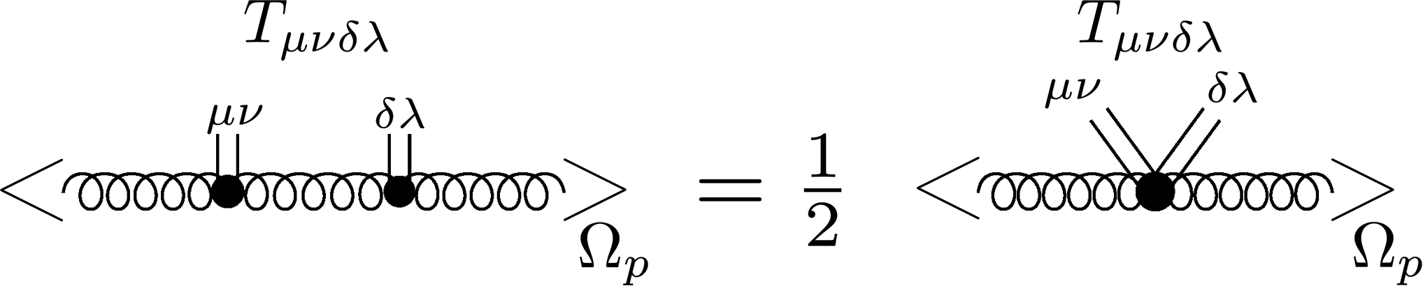
due to a non-trivial kinematic identity. This identity relates angular averages of one- and two-graviton–two-gluon scattering vertices in the absence of a gluon regulator $r_{a}$, see Fig.​ 2. In other words, for a combination of regulators that satisfy (38) the quantum-gauge and quantum-diffeomorphism symmetry violating effects of the regulators do not effect the kinematic identity that holds in the absence of the regulator.

This structure requires some care in the interpretation of the running of background observables for $k\to\infty$: while the physics properties of the dynamical fluctuation fields should not depend on the choice of the regulators, background observables do not necessarily display physics in this limit. By now we know of many examples for the latter deficiency ranging from the beta function of Yang-Mills theory, see [120], to the behaviour of the background couplings in pure gravity, [24, 26, 31, 61, 36] and matter-gravity systems [79, 82]. Moreover, we have already argued that the relation between the dynamical and the background minimal coupling only holds without modifications for sufficiently large momenta.

In summary, this implies the following for the interpretation of background observables: we either choose pairs of regulators that satisfy (38) or we evaluate background observables for momentum configurations that are not dominantly affected by the breaking of quantum-gauge and quantum-diffeomorphism invariance. Here, we will pursue the latter option that gives us more freedom in the choice of regulators. For the computation of the graviton contribution to the running of the Yang-Mills background coupling, this implies that we have to evaluate the flow of the two-point function for sufficiently large external momenta,

$\displaystyle p^{2}\gtrsim k^{2}\,.$

(39)

For these momenta, the three-point function diagrams effectively satisfy (38), and the anomalous dimension $\eta_{a,h}(p^{2})$ carries the information about the graviton contribution of the beta function of the background coupling.

The results of the discussion on background observables in the previous subsection IV.1 allow us to access the question of asymptotic freedom of the minimal Yang-Mills coupling. With the construction of the effective action (27), we obtain a flow equation for $\partial_{t}\Gamma^{(aa)}$, which is projected with the transverse projection operator

$\displaystyle P_{\mathrm{T}}^{\mu\nu}(p)=\delta^{\mu\nu}-\frac{p^{\mu}p^{\nu}}{p^{2}}\,.$

(40)

The graviton-induced contributions to the resulting flow equation take the form

	$\displaystyle P_{\mathrm{T}}^{\mu\nu}(p)\,$	$\displaystyle\partial_{t}\Gamma_{\mu\nu}^{(aa)}(p)=\mathrm{Flow}_{h}^{(aa)}(p^{2})=$
		$\displaystyle Z_{a}(p^{2})\,g\int_{q}\Big((\dot{r}(q^{2})-\eta_{a}(q^{2})r(q^{2}))f_{a}(q,p,\mu)$
		$\displaystyle\quad+(\dot{r}(q^{2})-\eta_{h}(q^{2})r(q^{2}))f_{h}(q,p,\mu)\Big)\,,$		(41)

where the terms on the right-hand side originate from diagrams with a regulator insertion in the gluon and graviton propagator, respectively. The left-hand side is simply given by

$\displaystyle P_{\mathrm{T}}^{\mu\nu}\,\partial_{t}\Gamma_{\mu\nu}^{(aa)}(p)=p^{2}\partial_{t}Z_{a}(p^{2})\,.$

(42)

Dividing by $Z_{a}(p^{2})$, one obtains an inhomogeneous Fredholm integral equation of the second kind for the gluon anomalous dimension,

$\displaystyle\eta_{a}(p^{2})=f(p^{2})+g\int\!\frac{\mathrm{d}^{4}q}{(2\pi)^{4}}\,K\!\left(p,q,\mu,\eta_{h}\right)\eta_{a}(q^{2})\,.$

(43)

This integral equation can be solved using the resolvent formalism by means of a Liouville-Neumann series. In this work we approximate the full momentum dependence by evaluating the anomalous dimension in the integrand in (43) at $q^{2}=k^{2}$. This is justified since the integrand is peaked at $q\approx k$ due to the regulator. With this approximation, (43) can be evaluated numerically for all momenta. This approximation was already used in [79] and lead to results in good qualitative agreement with the full momentum dependence. Details of the full solution are discussed in App. C. With the approximation to (43), we investigate the sign of the graviton contributions to the gluon propagator. These contributions are functions of the gravity couplings, which in turn depend on the truncation. It is therefore interesting to evaluate $\eta_{a,h}$ with a parametric dependence on the gravity couplings, in order to obtain general conditions under which asymptotic freedom is guaranteed.

The gluon anomalous dimension is of the form $\eta_{a}(p^{2},g,\mu,\eta_{h})$. In order to avoid the unphysical regulator dependence potentially induced by the violation of the kinematical identity (38) we choose the momentum $p^{2}=k^{2}$ in order to satisfy (39). In summary, this provides us with a minimal coupling $\alpha_{s}$,

$\displaystyle\partial_{t}\alpha_{s}=\beta_{\alpha_{s}}=\eta_{a}(k^{2})\,\alpha_{s}\,.$

(44)

As a main result in the present section, we conclude that

$\displaystyle\beta_{\alpha_{s}}\leq 0\qquad\text{for}\quad\mu>-1\quad\text{and}\quad\eta_{h}(k^{2})\leq 2\,.$

(45)

The restriction to $\eta_{h}\leq 2$ is also the bound on the anomalous dimension advocated in [79]. To be more precise, $\eta_{h}>2$ only changes the sign of the Yang-Mills beta function in the limit $\mu\to-1$. For other values of $\mu$, very large values of $\eta_{h}$ are necessary in order to destroy asymptotic freedom, e.g. for $\mu=-0.4$ the bound is $\eta_{h}\approx 50$ . The precise bound is displayed in Fig.​ 4, where the red region indicates $\beta_{\alpha_{s}}>0$.

Despite the necessary restriction to momenta $p^{2}\gtrsim k^{2}$ for its relation to the physical background coupling, we have also evaluated $\eta_{a,h}$ for more general momentum configurations and a range of gravity parameters $\mu$ and $\eta_{h}$: in Fig.​ 3, the sign of the graviton-induced part of the gluon anomalous dimension $\eta_{a,h}$ is plotted in the momentum range $0\leq p^{2}\leq k^{2}$. For small momenta, $\eta_{a,h}$ changes sign for $\mu\to-1$. Again it can be shown that this does not happen for regulators with (38).

In order to understand the patterns behind Fig.​ 3 and Fig.​ 4 it is illuminating to examine $\eta_{a,h}(p^{2}=0)$ for flat regulators (74) with a $p^{2}$ derivative. It reads

$\displaystyle\eta_{a,h}=-\frac{g}{8\pi}\left(\frac{8-\eta_{a}}{1+\mu}-\frac{4-\eta_{h}}{(1+\mu)^{2}}\right)\,.$

(46)

The first term on the right-hand side stems from $\partial_{t}R_{k,a}$ and is positive for $\eta_{a}<8$. The second stems from $\partial_{t}R_{h,k}$. It is non-vanishing for $\eta_{h}=0$ and hence already contributes at one-loop order. Its very presence reflects the breaking of the non-trivial kinematical identity depicted in Fig.​ 2 as it is proportional to it. The interpretation of $\eta_{a,h}$ as the graviton-induced running of the Yang-Mills background coupling crucially hinges on physical quantum gauge invariance: it is important to realise that only with the relation between the auxiliary background gauge invariance and quantum gauge invariance the latter carries physics. In turn, in the momentum regime where the kinematical identity is violated, physical gauge invariance is not guaranteed, and background gauge invariance reduces to an auxiliary symmetry with no physical content. Accordingly, one either has to evaluate $\eta_{a,h}(p^{2})$ for sufficiently large momenta $p^{2}\gtrsim k^{2}$ or utilises regulators that keep the kinematical identity Fig.​ 2 at least approximately for all momenta.

In summary, Fig.​ 3 and Fig.​ 4 entail that $\mathrm{sgn}(\eta_{a,h})<0$ holds for physically relevant momenta and values of the gravity couplings. Thus asymptotic freedom is preserved. We have argued that (44) provides the correct definition for the beta function of the minimal coupling of Yang-Mills theory with ${\rm sgn}(\beta_{\alpha_{s}})\leq 0$. Hence we conclude that an ultraviolet fixed point in the spirit of the asymptotic safety scenario is compatible with asymptotic freedom of the minimal coupling in Yang-Mills theories. In App. D, we utilise different approximations to the gluon anomalous dimension, and we discus in detail the regimes where it changes the sign in the parameter space of the gravity couplings.

For the question of asymptotic safety, we have to investigate the gluon contributions to the graviton propagator as well as to the graviton three-point function. This allows us to compute the corrections to the running of the gravity couplings $(\mu,g,\lambda_{3})$ due to gluon fluctuations.

The gluon corrections to the graviton two- and three-point function split analogously to the graviton corrections to Yang-Mills theory in the preceding section, since for any graviton $n$-point function the structure is given by

$\displaystyle\mathrm{Flow}^{(nh)}=\mathrm{Flow}^{(nh)}_{h}+\mathrm{Flow}^{(nh)}_{a}\,,$

(47)

with graviton and gluon contributions denoted by $\mathrm{Flow}^{(nh)}_{h}$ and $\mathrm{Flow}^{(nh)}_{a}$, respectively. For example, the gluon contributions to the flow of the graviton two- and three-point function are depicted in Fig.​ 5 and Fig.​ 6. Accordingly, the beta function for Newton’s coupling including gluon corrections has the structure

	$\displaystyle\partial_{t}g={}$	$\displaystyle\left(2+3\eta_{h}\right)g$		(48)
		$\displaystyle+g^{2}\Bigl(A_{h}(\mu,\lambda_{3})+\eta_{h}B_{h}(\mu,\lambda_{3})+C_{a}+\eta_{a}D_{a}\Bigr)\,,$

where we have used the identifications (25). In (48), $A_{h}$ and $B_{h}$ originate from graviton loops and they depend on $\mu$ and $\lambda_{3}$, while $C_{a}$ and $D_{a}$ are generated by gluon loops and are just numbers. Similarly the beta function for $\lambda_{3}$ has the structure

	$\displaystyle\partial_{t}\lambda_{3}={}$	$\displaystyle\left(-1+\frac{2}{3}\eta_{h}+\frac{\partial_{t}g}{2g}\right)\lambda_{3}$		(49)
		$\displaystyle+g\Bigl(E_{h}(\mu,\lambda_{3})+\eta_{h}F_{h}(\mu,\lambda_{3})+G_{a}+\eta_{a}H_{a}\Bigr)\,.$

Throughout this chapter we display the anomalous dimensions $\eta_{h},\eta_{a}$ as momentum independent. Note, however, that they are momentum dependent and we approximate their momentum dependence by evaluating them at $p=k$ if they appear in an integral, see [79] for details.

Moreover, the Yang-Mills contributions to the graviton propagator enter the above beta function (48) via the graviton anomalous dimension $\eta_{h}$ and the graviton mass parameter $\mu$. These equations have the general form

	$\displaystyle\eta_{h}={}$	$\displaystyle g\Bigl(I_{h}(\mu,\lambda_{3})+\eta_{h}J_{h}(\mu,\lambda_{3})+K_{a}+\eta_{a}L_{a}\Bigr)\,,$
	$\displaystyle\partial_{t}\mu={}$	$\displaystyle(\eta_{h}-2)\mu$		(50)
		$\displaystyle\,+g\Bigl(M_{h}(\mu,\lambda_{3})+N_{h}(\mu,\lambda_{3})\eta_{h}+O_{a}+\eta_{a}P_{a}\Bigr)\,,$

where again all pure gravity contributions are labelled with an index $h$ and the one generated by gluons with an index $a$. Note again that all the Yang-Mills contributions do not depend on $\mu$ and $\lambda_{3}$, as the corresponding diagrams do not involve graviton propagators and pure graviton vertices, see Fig.​ 5 and Fig.​ 6. In particular, this implies that these terms have no $1/(1+\mu)$ singularity in the limit $\mu\to-1$. Furthermore, all these diagrams contain a closed gluon loop, and hence, all the factors in the above equations with an index $a$ are proportional to $N^{2}_{c}-1$.

The gluon contribution to the graviton propagator has been studied in a derivative expansion around $p^{2}=0$ in [69] where it was shown that this projection is insufficient due to the non-trivial momentum dependence of the flow. The latter is characterized by a dip at $p^{2}\approx k^{2}$. It has been shown in [24] that this structure is also present in the full flow, i.e. including the graviton contributions and that projections at momentum scales close to the cutoff are necessary, see also [31, 36]. We have rederived the momentum dependence of $\mathrm{Flow}_{a}^{(2h)}(p^{2})$, see Fig.​ 7.

For the projection at $p^{2}=0$ and flat regulators (74), we rederive the result of [69] and obtain for the momentum-independent part

$\displaystyle\mathrm{Flow}_{a}^{(2h)}\left(p^{2}=0\right)=gZ_{h}(N_{c}^{2}-1)\frac{1}{60\pi}\eta_{a}\,.$

(51)

Surprisingly, this contribution is proportional to $\eta_{a}$. This happens due to a cancellation between both diagrams displayed in Fig.​ 5. Note that this cancellation only occurs for the flat regulator. For other regulators the contribution can be either positive or negative. This is discussed in App. B and will play a crucial rôle in the later analysis.

For the computation of the graviton anomalous dimension, we resort to a finite difference projection, which is of the general form

$\displaystyle\frac{\mathrm{Flow}_{a}^{(2h)}({p^{2}_{1}})-\mathrm{Flow}^{(2h)}_{a}({p^{2}_{2}})}{p^{2}_{1}-p^{2}_{2}}=gZ_{h}(N_{c}^{2}-1)(\alpha+\beta\,\eta_{a})\,,$

(52)

where $\alpha$ and $\beta$ depend only on $p_{1}$ and $p_{2}$. This is rooted in the fact that there are only internal gluon propagators and graviton-gluon vertices, and these do not depend on $\lambda_{3}$ and $\mu$ as discussed in the last section. For $p_{2}=0$ and $p_{1}\rightarrow p_{2}$, i.e. a $p^{2}$-derivative at $p^{2}=0$, we obtain

$\displaystyle\alpha=\beta=-\frac{1}{12\pi}\approx-0.027\,.$

(53)

For a finite difference with $p^{2}_{1}=k^{2}$ and $p_{2}=0$, we obtain

$\displaystyle\alpha\approx-0.012\,,\qquad\qquad\beta\approx-0.0033\,.$

(54)

(53) and (54) display the gluon contribution to $-\eta_{h}$; thus, the gluon contribution to $\eta_{h}$ is positive independent of the momentum projection scheme. Note however that (53) and (54) display a qualitatively different behaviour, and (54) is the correct choice due to the momentum dependence of the flow. This has already been observed in the pure gravity computations in [24, 26, 31, 36] and emphasises the importance of the momentum-dependence. In this work we use a finite difference between $p^{2}_{1}=p^{2}$ and $p^{2}_{2}=-\mu k^{2}$ for the equation of $\eta_{h}(p^{2})$, see [26, 79] for details.

References

- [1] S. Weinberg, General Relativity: An Einstein centenary survey, Eds. Hawking, S.W., Israel, W; Cambridge University Press , 790 (1979).
- [2] M. Reuter, Phys. Rev. D57, 971 (1998), arXiv:hep-th/9605030 .
- [3] M. Niedermaier, Class. Quant. Grav. 24, R171 (2007), arXiv:gr-qc/0610018 .
- [4] D. F. Litim, AIP Conf.Proc. 841, 322 (2006), arXiv:hep-th/0606044 [hep-th] .
- [5] R. Percacci, In *Oriti, D. (ed.): Approaches to quantum gravity* 111-128 (2007), arXiv:0709.3851 [hep-th] .
- [6] D. F. Litim, Proceedings, Workshop on From quantum to emergent gravity: Theory and phenomenology (QG-Ph): Trieste, Italy, June 11-15, 2007, (2008), [PoSQG-Ph,024(2007)], arXiv:0810.3675 [hep-th] .
- [7] D. F. Litim, Phil.Trans.Roy.Soc.Lond. A369, 2759 (2011), arXiv:1102.4624 [hep-th] .
- [8] M. Reuter and F. Saueressig, New J. Phys. 14, 055022 (2012), arXiv:1202.2274 [hep-th] .
- [9] W. Souma, Prog.Theor.Phys. 102, 181 (1999), arXiv:hep-th/9907027 [hep-th] .
- [10] S. Falkenberg and S. D. Odintsov, Int.J.Mod.Phys. A13, 607 (1998), arXiv:hep-th/9612019 [hep-th] .
- [11] M. Reuter and F. Saueressig, Phys. Rev. D65, 065016 (2002), arXiv:hep-th/0110054 [hep-th] .
- [12] O. Lauscher and M. Reuter, Phys. Rev. D65, 025013 (2002a), arXiv:hep-th/0108040 .
- [13] D. F. Litim, Phys.Rev.Lett. 92, 201301 (2004), arXiv:hep-th/0312114 [hep-th] .
- [14] A. Bonanno and M. Reuter, JHEP 02, 035 (2005), arXiv:hep-th/0410191 [hep-th] .
- [15] P. Fischer and D. F. Litim, Phys.Lett. B638, 497 (2006), arXiv:hep-th/0602203 [hep-th] .
- [16] A. Eichhorn, H. Gies, and M. M. Scherer, Phys. Rev. D80, 104003 (2009), arXiv:0907.1828 [hep-th] .
- [17] E. Manrique and M. Reuter, Annals Phys. 325, 785 (2010), arXiv:0907.2617 [gr-qc] .
- [18] A. Eichhorn and H. Gies, Phys. Rev. D81, 104010 (2010), arXiv:1001.5033 [hep-th] .
- [19] K. Groh and F. Saueressig, J. Phys. A43, 365403 (2010), arXiv:1001.5032 [hep-th] .
- [20] E. Manrique, M. Reuter, and F. Saueressig, Annals Phys. 326, 463 (2011a), arXiv:1006.0099 [hep-th] .
- [21] E. Manrique, S. Rechenberger, and F. Saueressig, Phys.Rev.Lett. 106, 251302 (2011b), arXiv:1102.5012 [hep-th] .
- [22] D. Litim and A. Satz, (2012), arXiv:1205.4218 [hep-th] .
- [23] I. Donkin and J. M. Pawlowski, (2012), arXiv:1203.4207 [hep-th] .
- [24] N. Christiansen, D. F. Litim, J. M. Pawlowski, and A. Rodigast, Phys.Lett. B728, 114 (2014), arXiv:1209.4038 [hep-th] .
- [25] A. Codello, G. D’Odorico, and C. Pagani, Phys. Rev. D89, 081701 (2014), arXiv:1304.4777 [gr-qc] .
- [26] N. Christiansen, B. Knorr, J. M. Pawlowski, and A. Rodigast, Phys. Rev. D93, 044036 (2016), arXiv:1403.1232 [hep-th] .
- [27] D. Becker and M. Reuter, Annals Phys. 350, 225 (2014), arXiv:1404.4537 [hep-th] .
- [28] K. Falls, JHEP 01, 069 (2016), arXiv:1408.0276 [hep-th] .
- [29] K. Falls, Phys. Rev. D92, 124057 (2015a), arXiv:1501.05331 [hep-th] .
- [30] K. Falls, (2015b), arXiv:1503.06233 [hep-th] .
- [31] N. Christiansen, B. Knorr, J. Meibohm, J. M. Pawlowski, and M. Reichert, Phys. Rev. D92, 121501 (2015), arXiv:1506.07016 [hep-th] .
- [32] H. Gies, B. Knorr, and S. Lippoldt, Phys. Rev. D92, 084020 (2015), arXiv:1507.08859 [hep-th] .
- [33] D. Benedetti, Gen. Rel. Grav. 48, 68 (2016), arXiv:1511.06560 [hep-th] .
- [34] J. Biemans, A. Platania, and F. Saueressig, Phys. Rev. D95, 086013 (2017a), arXiv:1609.04813 [hep-th] .
- [35] C. Pagani and M. Reuter, Phys. Rev. D95, 066002 (2017), arXiv:1611.06522 [gr-qc] .
- [36] T. Denz, J. M. Pawlowski, and M. Reichert, Eur. Phys. J. C78, 336 (2018), arXiv:1612.07315 [hep-th] .
- [37] K. Falls, Phys. Rev. D96, 126016 (2017), arXiv:1702.03577 [hep-th] .
- [38] W. B. Houthoff, A. Kurov, and F. Saueressig, Eur. Phys. J. C77, 491 (2017), arXiv:1705.01848 [hep-th] .
- [39] B. Knorr and S. Lippoldt, Phys. Rev. D96, 065020 (2017), arXiv:1707.01397 [hep-th] .
- [40] O. Lauscher and M. Reuter, Phys. Rev. D66, 025026 (2002b), arXiv:hep-th/0205062 .
- [41] A. Codello and R. Percacci, Phys. Rev. Lett. 97, 221301 (2006), arXiv:hep-th/0607128 .
- [42] A. Codello, R. Percacci, and C. Rahmede, Int. J. Mod. Phys. A23, 143 (2008), arXiv:0705.1769 [hep-th] .
- [43] P. F. Machado and F. Saueressig, Phys. Rev. D77, 124045 (2008), arXiv:0712.0445 [hep-th] .
- [44] A. Codello, R. Percacci, and C. Rahmede, Annals Phys. 324, 414 (2009), arXiv:0805.2909 [hep-th] .
- [45] M. R. Niedermaier, Phys. Rev. Lett. 103, 101303 (2009).
- [46] D. Benedetti, P. F. Machado, and F. Saueressig, Mod. Phys. Lett. A24, 2233 (2009), arXiv:0901.2984 [hep-th] .
- [47] S. Rechenberger and F. Saueressig, Phys.Rev. D86, 024018 (2012), arXiv:1206.0657 [hep-th] .
- [48] D. Benedetti and F. Caravelli, JHEP 06, 017 (2012), [Erratum: JHEP10,157(2012)], arXiv:1204.3541 [hep-th] .
- [49] J. A. Dietz and T. R. Morris, JHEP 01, 108 (2013a), arXiv:1211.0955 [hep-th] .
- [50] N. Ohta and R. Percacci, Class. Quant. Grav. 31, 015024 (2014), arXiv:1308.3398 [hep-th] .
- [51] K. Falls, D. Litim, K. Nikolakopoulos, and C. Rahmede, (2013), arXiv:1301.4191 [hep-th] .
- [52] D. Benedetti, Europhys. Lett. 102, 20007 (2013), arXiv:1301.4422 [hep-th] .
- [53] J. A. Dietz and T. R. Morris, JHEP 07, 064 (2013b), arXiv:1306.1223 [hep-th] .
- [54] K. Falls, D. F. Litim, K. Nikolakopoulos, and C. Rahmede, Phys. Rev. D93, 104022 (2016), arXiv:1410.4815 [hep-th] .
- [55] A. Eichhorn, JHEP 04, 096 (2015), arXiv:1501.05848 [gr-qc] .
- [56] N. Ohta, R. Percacci, and G. P. Vacca, Phys. Rev. D92, 061501 (2015), arXiv:1507.00968 [hep-th] .
- [57] N. Ohta, R. Percacci, and G. P. Vacca, Eur. Phys. J. C76, 46 (2016), arXiv:1511.09393 [hep-th] .
- [58] K. Falls, D. F. Litim, K. Nikolakopoulos, and C. Rahmede, Class. Quant. Grav. 35, 135006 (2018), arXiv:1607.04962 [gr-qc] .
- [59] K. Falls and N. Ohta, Phys. Rev. D94, 084005 (2016), arXiv:1607.08460 [hep-th] .
- [60] H. Gies, B. Knorr, S. Lippoldt, and F. Saueressig, Phys. Rev. Lett. 116, 211302 (2016), arXiv:1601.01800 [hep-th] .
- [61] N. Christiansen, (2016), arXiv:1612.06223 [hep-th] .
- [62] S. Gonzalez-Martin, T. R. Morris, and Z. H. Slade, Phys. Rev. D95, 106010 (2017), arXiv:1704.08873 [hep-th] .
- [63] D. Becker, C. Ripken, and F. Saueressig, JHEP 12, 121 (2017), arXiv:1709.09098 [hep-th] .
- [64] D. Dou and R. Percacci, Class. Quant. Grav. 15, 3449 (1998), arXiv:hep-th/9707239 [hep-th] .
- [65] R. Percacci and D. Perini, Phys. Rev. D67, 081503 (2003), arXiv:hep-th/0207033 .
- [66] G. Narain and R. Percacci, Class. Quant. Grav. 27, 075001 (2010), arXiv:0911.0386 [hep-th] .
- [67] J. E. Daum, U. Harst, and M. Reuter, Gen. Relativ. Gravit. (2010), 10.1007/s10714-010-1032-2, [Gen. Rel. Grav.43,2393(2011)], arXiv:1005.1488 [hep-th] .
- [68] S. Folkerts, D. F. Litim, and J. M. Pawlowski, Phys.Lett. B709, 234 (2012), arXiv:1101.5552 [hep-th] .
- [69] S. Folkerts, Diploma thesis, Heidelberg (2009).
- [70] U. Harst and M. Reuter, JHEP 05, 119 (2011), arXiv:1101.6007 [hep-th] .
- [71] A. Eichhorn and H. Gies, New J. Phys. 13, 125012 (2011), arXiv:1104.5366 [hep-th] .
- [72] A. Eichhorn, Phys. Rev. D86, 105021 (2012), arXiv:1204.0965 [gr-qc] .
- [73] P. Donà and R. Percacci, Phys. Rev. D87, 045002 (2013), arXiv:1209.3649 [hep-th] .
- [74] T. Henz, J. M. Pawlowski, A. Rodigast, and C. Wetterich, Phys. Lett. B727, 298 (2013), arXiv:1304.7743 [hep-th] .
- [75] P. Donà, A. Eichhorn, and R. Percacci, Phys.Rev. D89, 084035 (2014), arXiv:1311.2898 [hep-th] .
- [76] R. Percacci and G. P. Vacca, Eur. Phys. J. C75, 188 (2015), arXiv:1501.00888 [hep-th] .
- [77] P. Labus, R. Percacci, and G. P. Vacca, Phys. Lett. B753, 274 (2016), arXiv:1505.05393 [hep-th] .
- [78] K.-y. Oda and M. Yamada, Class. Quant. Grav. 33, 125011 (2016), arXiv:1510.03734 [hep-th] .
- [79] J. Meibohm, J. M. Pawlowski, and M. Reichert, Phys. Rev. D93, 084035 (2016), arXiv:1510.07018 [hep-th] .
- [80] P. Donà, A. Eichhorn, P. Labus, and R. Percacci, Phys. Rev. D93, 044049 (2016), [Erratum: Phys. Rev.D93,no.12,129904(2016)], arXiv:1512.01589 [gr-qc] .
- [81] J. Meibohm and J. M. Pawlowski, Eur. Phys. J. C76, 285 (2016), arXiv:1601.04597 [hep-th] .
- [82] A. Eichhorn, A. Held, and J. M. Pawlowski, Phys. Rev. D94, 104027 (2016), arXiv:1604.02041 [hep-th] .
- [83] T. Henz, J. M. Pawlowski, and C. Wetterich, Phys. Lett. B769, 105 (2017), arXiv:1605.01858 [hep-th] .
- [84] A. Eichhorn and S. Lippoldt, Phys. Lett. B767, 142 (2017), arXiv:1611.05878 [gr-qc] .
- [85] N. Christiansen and A. Eichhorn, Phys. Lett. B770, 154 (2017), arXiv:1702.07724 [hep-th] .
- [86] A. Eichhorn and A. Held, Phys. Rev. D96, 086025 (2017), arXiv:1705.02342 [gr-qc] .
- [87] J. Biemans, A. Platania, and F. Saueressig, JHEP 05, 093 (2017b), arXiv:1702.06539 [hep-th] .
- [88] N. Christiansen, A. Eichhorn, and A. Held, Phys. Rev. D96, 084021 (2017), arXiv:1705.01858 [hep-th] .
- [89] A. Eichhorn and A. Held, Phys. Lett. B777, 217 (2018), arXiv:1707.01107 [hep-th] .
- [90] A. Eichhorn and F. Versteegen, JHEP 01, 030 (2018), arXiv:1709.07252 [hep-th] .
- [91] A. Eichhorn, in Black Holes, Gravitational Waves and Spacetime Singularities Rome, Italy, May 9-12, 2017 (2017) arXiv:1709.03696 [gr-qc] .
- [92] N. Alkofer and F. Saueressig, (2018), arXiv:1802.00498 [hep-th] .
- [93] S. P. Robinson and F. Wilczek, Phys. Rev. Lett. 96, 231601 (2006), arXiv:hep-th/0509050 .
- [94] A. R. Pietrykowski, Phys. Rev. Lett. 98, 061801 (2007), arXiv:hep-th/0606208 .
- [95] D. J. Toms, Phys. Rev. D76, 045015 (2007), arXiv:0708.2990 [hep-th] .
- [96] D. Ebert, J. Plefka, and A. Rodigast, Phys. Lett. B660, 579 (2008), arXiv:0710.1002 [hep-th] .
- [97] Y. Tang and Y.-L. Wu, Commun. Theor. Phys. 54, 1040 (2010), arXiv:0807.0331 [hep-ph] .
- [98] D. J. Toms, Nature 468, 56 (2010), arXiv:1010.0793 [hep-th] .
- [99] J. F. Donoghue, Phys. Rev. Lett. 72, 2996 (1994), arXiv:gr-qc/9310024 .
- [100] D. F. Litim and J. M. Pawlowski, Phys.Lett. B435, 181 (1998), arXiv:hep-th/9802064 [hep-th] .
- [101] D. F. Litim and F. Sannino, JHEP 12, 178 (2014), arXiv:1406.2337 [hep-th] .
- [102] D. F. Litim, M. Mojaza, and F. Sannino, JHEP 01, 081 (2016), arXiv:1501.03061 [hep-th] .
- [103] A. D. Bond and D. F. Litim, Eur. Phys. J. C77, 429 (2017a), arXiv:1608.00519 [hep-th] .
- [104] A. D. Bond, G. Hiller, K. Kowalska, and D. F. Litim, JHEP 08, 004 (2017), arXiv:1702.01727 [hep-ph] .
- [105] A. D. Bond and D. F. Litim, Phys. Rev. D97, 085008 (2018), arXiv:1707.04217 [hep-th] .
- [106] A. D. Bond and D. F. Litim, Phys. Rev. Lett. 119, 211601 (2017b), arXiv:1709.06953 [hep-th] .
- [107] D. F. Litim and J. M. Pawlowski, Phys.Rev. D66, 025030 (2002a), arXiv:hep-th/0202188 [hep-th] .
- [108] D. F. Litim and J. M. Pawlowski, Phys.Lett. B546, 279 (2002b), arXiv:hep-th/0208216 [hep-th] .
- [109] A. K. Cyrol, L. Fister, M. Mitter, J. M. Pawlowski, and N. Strodthoff, Phys. Rev. D94, 054005 (2016), arXiv:1605.01856 [hep-ph] .
- [110] A. K. Cyrol, M. Mitter, J. M. Pawlowski, and N. Strodthoff, Phys. Rev. D97, 054006 (2018), arXiv:1706.06326 [hep-ph] .
- [111] A. Eichhorn, H. Gies, and J. M. Pawlowski, Phys.Rev. D83, 045014 (2011), arXiv:1010.2153 [hep-ph] .
- [112] S. Diehl, H. C. Krahl, and M. Scherer, Phys. Rev. C78, 034001 (2008), arXiv:0712.2846 [cond-mat.stat-mech] .
- [113] J. M. Pawlowski, M. M. Scherer, R. Schmidt, and S. J. Wetzel, Annals Phys. 384, 165 (2017), arXiv:1512.03598 [hep-th] .
- [114] C. Wetterich, Phys. Lett. B301, 90 (1993), arXiv:1710.05815 [hep-th] .
- [115] U. Ellwanger, Proceedings, Workshop on Quantum field theoretical aspects of high energy physics: Bad Frankenhausen, Germany, September 20-24, 1993, Z. Phys. C62, 503 (1994), arXiv:hep-ph/9308260 [hep-ph] .
- [116] T. R. Morris, Int. J. Mod. Phys. A9, 2411 (1994), arXiv:hep-ph/9308265 .
- [117] D. F. Litim, Phys.Lett. B486, 92 (2000), arXiv:hep-th/0005245 [hep-th] .
- [118] D. F. Litim, Phys.Rev. D64, 105007 (2001a), arXiv:hep-th/0103195 [hep-th] .
- [119] F. Freire, D. F. Litim, and J. M. Pawlowski, Phys.Lett. B495, 256 (2000), arXiv:hep-th/0009110 [hep-th] .
- [120] D. F. Litim and J. M. Pawlowski, JHEP 09, 049 (2002c), arXiv:hep-th/0203005 [hep-th] .
- [121] J. M. Pawlowski, (2003), arXiv:hep-th/0310018 [hep-th] .
- [122] J. M. Pawlowski, Annals Phys. 322, 2831 (2007), arXiv:hep-th/0512261 [hep-th] .
- [123] D. F. Litim, Int.J.Mod.Phys. A16, 2081 (2001b), arXiv:hep-th/0104221 [hep-th] .
- [124] D. F. Litim and J. M. Pawlowski, JHEP 0611, 026 (2006), arXiv:hep-th/0609122 [hep-th] .
- [125] D. F. Litim, Nucl.Phys. B631, 128 (2002), arXiv:hep-th/0203006 [hep-th] .
- [126] D. F. Litim, Phys.Rev. D76, 105001 (2007), arXiv:0704.1514 [hep-th] .
- [127] H. Bückner et al., Duke Mathematical Journal 15, 197 (1948).
- [128] J. A. M. Vermaseren, (2000), arXiv:math-ph/0010025 [math-ph] .
- [129] J. Kuipers, T. Ueda, J. A. M. Vermaseren, and J. Vollinga, Comput. Phys. Commun. 184, 1453 (2013), arXiv:1203.6543 [cs.SC] .
- [130] D. Brizuela, J. M. Martin-Garcia, and G. A. Mena Marugan, Gen. Rel. Grav. 41, 2415 (2009), arXiv:0807.0824 [gr-qc] .
- [131] A. K. Cyrol, M. Mitter, and N. Strodthoff, Comput. Phys. Commun. 219, 346 (2017), arXiv:1610.09331 [hep-ph] .