Linear Programming Bounds for Distributed Storage CodesThanks: This work was partially supported by a grant from Australian Research Council (DP1094571) and the University Grants Committee of the Hong Kong Special Administrative Region, China (Project No. AoE/E-02/08).
Abstract.
A major issue of locally repairable codes is their robustness. If a local repair group is not able to perform the repair process, this will result in increasing the repair cost. Therefore, it is critical for a locally repairable code to have multiple repair groups. In this paper we consider robust locally repairable coding schemes which guarantee that there exist multiple distinct (not necessarily disjoint) alternative local repair groups for any single failure such that the failed node can still be repaired locally even if some of the repair groups are not available. We use linear programming techniques to establish upper bounds on the code size of these codes. We also provide two examples of robust locally repairable codes that are optimal regarding our linear programming bound. Furthermore, we address the update efficiency problem of the distributed data storage networks. Any modification on the stored data will result in updating the content of the storage nodes. Therefore, it is essential to minimise the number of nodes which need to be updated by any change in the stored data. We characterise the update-efficient storage code properties and establish the necessary conditions of existence update-efficient locally repairable storage codes.
Key words and phrases:
Distributed storage network, erasure code, linear programming, locally repairable code, update complexity1991 Mathematics Subject Classification
Primary: 68P20, 94B05, 68P30; Secondary: 90C05.Ali Tebbi
Institute for Telecommunications Research
University of South Australia
Terence Chan∗ and Chi Wan Sung∗∗
∗Institute for Telecommunications Research
University of South Australia
∗∗Department of Electronic Engineering
City University of Hong Kong
(Communicated by the associate editor name)
1. Introduction
Significant increase in the internet applications such as social networks, file, and video sharing applications, results in an enormous user data production which needs to be stored reliably. In a data storage network, data is usually stored in several data centres, which can be geographically separated. Each data centre can store a massive amount of data, by using hundreds of thousands of storage disks (or nodes). The most common issue with all storage networks is failure. The failure in storage networks is the result of the failed components which are varied from corrupted disk sectors to one or a group of failed disks or even the entire data centre due to the physical damages or natural disasters. The immediate consequence of failure in a storage network is data loss. Therefore, a repair mechanism must be in place to handle these failures. Protection against failures is usually achieved by adding redundancies [24]. The simplest way to introduce redundancy is replication. In this method multiple copies of each data block are stored in the network. In the case of any failure in the network, the content of the failed node can be recovered by its replica. Because of its simplicity in storage and data retrieval, this method is used widely in conventional storage systems (e.g., RAID-1 where each data block is duplicated and stored in two storage nodes) [6, 14]. However, replication is not an efficient method in term of the storage requirement [12, 35].
Another method for data storage is erasure coding which has gained a wide attention in distributed storage [30, 23, 2, 3, 4]. In this method as a generalisation of replication, a data block is divided into fragments and then encoded to () fragments via a group of mapping functions to store in the network [42]. Erasure coding is capable of providing more reliable storage networks compared to replication with the same storage overhead [41]. It is noteworthy to mention that replication can also be considered as an erasure code (i.e., repetition code [24]).
One of the challenges in storage networks using erasure codes is the repair bandwidth. When a storage node fails, the replaced node (i.e., newcomer) has to download the information content of the survived nodes to repair the lost data. In other words, the repair bandwidth of a distributed storage network is the total amount of the information which is needed to be retrieved to recover the lost data. Compared to the replication, It has been shown in [41] that in the systems with the same mean time to failure (MTTF), using erasure codes reduces the storage overhead and the repair bandwidth by an order of magnitude.
From coding theory, it is well known that in a storage network employing an erasure code for data storage the minimum amount of information which has to be downloaded to repair a single failure is at least the same size of the original data [42]. In other words, the amount of data transmitted in the network to repair a failed node is much more than the storage capacity of the node. Regenerating codes which have been introduced in [13] provide coding techniques to reduce the repair bandwidth by increasing the number of nodes which the failed node has to be connected during the repair procedure. It has been shown that there exists a tradeoff between the storage and repair bandwidth in distributed storage networks [13]. Many storage codes in literature assume that lost data in a failed data centre can be regenerated from any subset (of size greater than a certain threshold) of surviving data centres. This requirement can be too restrictive and sometimes not necessary. Although these methods reduce the repair bandwidth, minimising I/O in distributed storage networks is more beneficial than minimising the repair bandwidth [22]. Storage codes such as regenerating codes that access all surviving nodes during repair process, increase I/O overhead. Disk I/O which is proportional to the number of the nodes involved in the repair process, seems to be the repair performance bottleneck of the storage networks [28].
The number of nodes which involve in repairing a failed node is defined as the code locality [17]. The concept of code locality relaxes the repairing requirement so that any failed node can be repaired by at least one set (of size smaller than a threshold) of surviving nodes. We refer to these sets as local repair groups. Moreover, any erasure code which satisfies this property is referred as locally repairable code.
One significant issue of locally repairable codes is their robustness. Consider a distributed storage network with storage nodes such that there exists only one local repair group for each node in the network. Therefore, if any node fails, the survived nodes in its repair group can locally repair the failure. However, if any other node in the repair group is also not available (for example, due to the heavy loading), then the repair group cannot be able to repair the failed node anymore which will result in an increase of repair cost. To avoid this problem, it is essential to have multiple local repair groups which can be used for repairing the failure if additional nodes fail or become unavailable in the repair groups. The concept of locally repairable codes with multiple repair groups (or alternatives) was studied in [27] where codes with multiple repair alternatives were also constructed. Locally repairable code construction with multiple disjoint repairing groups was investigated in [34]. Locally repairable codes with multiple erasure tolerance are introduced in [21] where any failed node can be locally repaired even in the presence of multiple erasures. In [40], locally repairable codes with multiple erasure tolerance have been constructed using combinatorial methods. A lower bound on the code size was derived and some code examples provided which are optimal with respect to this bound. A class of locally repairable codes with capability of repairing a set of failed nodes by connecting to a set of survived nodes are studied in [33]. Bounds on code dimension and also families of explicit codes were provided.
The main contributions of this paper are as follows:
- •
We investigate the linear robust locally repairable codes, defined in Definition 3.4, where any failed node can be repaired by different (i.e., distinct but not necessarily disjoint) repair groups each of size at most at the presence of any extra failures in the network. These codes have a minimum distance of , i.e., these codes can tolerate any simultaneous failures.
- •
By employing the criteria from the definition of our robust locally repairable codes, we establish a linear programming bound to upper bound the code size.
- •
We propose two robust locally repairable code examples which are optimal regarding our linear programming bound.
- •
We investigate the update efficiency of storage codes. In an erasure code, each encoded symbol is a function of the data symbols. Therefore, the update complexity of an erasure code is proportional to the number of encoded symbols that have to be changed in regard of any change in the original data symbols. In other words, in a storage network the content of the storage nodes must be updated by any change in the stored data. We characterise the properties of update-efficient storage codes and establish the necessary conditions that the codes need to satisfy.
Our linear programming bounds are alphabet dependant and establish upper bounds on the code size for arbitrary code parameters such as code length, minimum distance, local repair group’s size, number of the local repair groups, and number of the failed nodes in the network. The significance of our linear programming bounds compared to the similar approaches (e.g., [8] or [1]) is that our bounds can be easily generalised for different variations of linear storage codes such that any criterion can be presented as a linear constraint in the problem. Moreover, the complexity of these problems can be significantly reduced by applying symmetries of the codes.
This work is partially presented in 2013 9th International Conference on Information, Communications & Signal Processing (ICICS) [10] and 2014 IEEE Information Theory Workshop (ITW) [39]. This work presents more detailed discussions on characterising robust locally repairable and update-efficient storage codes.
The remaining of the paper is organised as follows. In Section 2, we review the related works on the locally repairable codes. In Section 3, we introduce our robust locally repairable codes and propose their criteria. In Section 4, we establish a linear programming problem to upper bound the code size. We also exploit symmetry on the linear programming bound to reduce its complexity. Section 5 studies the update efficiency of the locally repairable codes. We establish the necessary conditions for distributed storage codes in order to satisfy the locality and update efficiency at the same time. Examples and numerical results are provided in Section 6. The paper then concludes in Section 7.
2. Background and Related Works
Disk I/O which is proportional to the number of the nodes involved in the repair process, seems to be the repair performance bottleneck of the storage networks [28]. Regenerating codes are an example of this issue where surviving nodes are involved in repair process of a failed node in order to minimise the repair bandwidth [22]. Therefore, the number of nodes which help to repair a failed node is a major metric to measure the repair cost in storage networks. Locally repairable codes aim to optimise this metric (i.e., the number of helper nodes needed to repair a failed node). The locality of a code is defined as the number of code coordinates such that any code coordinate is a function of them [17]. Consequently, in a storage network employing a locally repairable code, any failed node can be repaired using only survived nodes. In the case of the linear locally repairable storage codes which are the topic of this paper, the content of any storage node is a linear combination of the contents of a group of other nodes. Usually two types of code locality are defined in the literature as information symbol locality and all symbol locality which means that just the information symbols in a systematic code have locality and all symbols have locality , respectively. In this paper, the code locality is referred to all symbol locality since we do not impose any systematic code constraint on the locally repairable storage codes.
The problem of storage codes with small locality has been initially proposed in [18, 26, 29], independently. The Pyramid codes introduced in [18] are an example of initial works on practical locally repairable storage codes. A basic Pyramid code is constructed using an existing erasure code. An MDS erasure code will be an excellent choice in this case, since they are more tolerable against simultaneous failures. To construct a Pyramid code using an MDS code, it is sufficient to split data blocks into disjoint groups. Then, a parity symbol is calculated for each group as a local parity. In other words, one of the parity symbols from the original code is split into blocks and the other parity symbols are kept as global parities. Therefore, any single failure in data nodes can be repaired by survived nodes in the same group instead of retrieving data from nodes. Generally, for a Pyramid code with data locality constructed from an MDS code, the code length (i.e., number of storage nodes) is
| (1) |
Obviously, low locality is gained in the cost of extra storage. To obtain all symbol locality for the code, it is sufficient to add a local parity to each group of the global parities of size where will result in a code length of
| (2) |
Both of the code lengths in (1) and (2) show a linear increase in storage overhead. Note that in general, adding a local parity to each group will decrease the minimum distance of the code which is a major challenge in constructing optimal all-symbol locally repairable codes [37].
The pioneer work of Gopalan in [17] is an in-depth study of codes locality which results in presenting a trade-off between the code length , data block size , minimum distance of code , and code locality . It has been shown that for any linear code with information locality ,
| (3) |
In other words, to have a linear storage code with locality , we need a linear overhead of at least . As a special case of locality , the bound in (3) is reduced to
| (4) |
which is the Singleton bound and is achievable by MDS codes such as Reed-Solomon codes. According to (1) and (2), Pyramid codes can achieve the bound in (3) which shows their optimality.
Due to their importance in minimising the number of helper nodes to repair a single failure, locally repairable codes have received a fair amount of attention in literature. Different coding schemes to design explicit optimum locally repairable codes has been proposed in [38, 32, 37, 5, 16, 15, 25].
For the bound in (3), the assumption is that any storage node has entropy equal to , where is the data block size to be stored. It is also mentioned that low locality affects minimum distance regarding the term . It has been shown in [28] that there exist erasure codes which have high distance and low locality if storage nodes store an additional information by a factor of . The minimum distance of these codes is upper bounded as
| (5) |
where . The obtained LRCs in [28] are vector codes where each data and coded symbol is represented as a vector (not necessarily of the same length). The definition of the vector LRCs, together with the bound in (5), are extended to localities in [32] which we will describe later.
The main issue with locally repairable codes is that they mostly tend to repair a single node failure. This means that if any of the helper nodes in the repair group of a failed node is not available, the local repair process will fail. Therefore, it is critical to have multiple repair groups for each node in the storage network. The concept of locally repairable codes with multiple repair alternatives has been studied initially in [27]. The main idea in [27] is to obtain the parity check matrix of the code from a partial geometries. However, there are only a few such explicit codes due to the limited number of known constructions of partial geometries with desirable parameters. A lower and upper bound is also obtained for the rate of these codes with different locality and repair alternativity. Rawat et al. investigated the availability in storage networks employing locally repairable codes [34]. The notion of availability is useful for applications involving hot data since it gives the ability of accessing to a certain information by different users simultaneously. Therefore, each information node must have disjoint repair groups of size at most (i.e., -Information local code). An upper bound for the code minimum distance has been obtained in [34] as
| (6) |
which is a generalised version of the bound in (3). However, this bound only stands for information symbols availability with the assumption of only one parity symbol for each repair group. Different bounds on the rate and minimum distance of storage codes with locality and availability have been obtained independently in [36] as
| (7) |
and
| (8) |
The minimum distance upper bound in (8) reduces to (3) for . However, the bounds in (6) and (8) seem to be incomparable since the bound in (8) is tighter than (6) in some cases and vice versa.
An upper bound on the codebook size of locally repairable codes which is dependent on the alphabet size has been obtained in [7] as
| (9) |
where, is the maximum dimension of a linear or non-linear code of length and minimum distance with alphabet size of . This bound is tighter than the bound in (3).
Locally repairable codes with small availability are investigated in [20]. The smallest the availability the highest the code rate would be since the dependency among the code symbols is less while the code is still comparable to the practical replication codes. The rate optimal binary -availability codes are designed in [31].
-locally repairable codes are introduced in [21] where the failed coded symbols can be repaired locally by at most symbols at the presence of multiple failures in the network. The symbol , , of a code with minimum distance is said to have locality if there exists a subcode of with support containing whose length is at most and whose minimum distance is at least . For a systematic code with all information symbols locality, any systematic symbol can be repaired by other symbols even if there are extra failures. The minimum distance of these codes is upper bounded as
Partial MDS (PMDS) codes are introduced in [5]. A linear code is a -PMDS code where each row of the array belongs to an MDS code. PMDS codes combine local correction of errors in each row with global correction of erasures anywhere in the array. As mentioned earlier, in classes of locally repairable codes (e.g., PMDS codes or Pyramid codes) there are local parity symbols which depend only on a specific group of data symbols and some global parities which depend on all data symbols. While the local parities provide a fast repair of single failures, the global parities provide a high resilience against simultaneous failures. The codes described as above are called Maximally Recoverable (MR) [18] if they can repair all failure patterns which are information theoretically repairable. Families of explicit maximally recoverable codes with locality are proposed in [16]. PMDS codes and MR codes with locality are a class of -locally repairable codes that not only have optimal minimum distance, but can correct all information theoretically correctable erasure patterns for the given , code length and dimension .
A challenge to construct these type of optimal LRCs (e.g., PMDS codes) is to obtain small field sizes. An exponential field size of is obtained in [9] for PMDS codes with arbitrary and . The authors in [15], extend the work in [16] for to obtain a relatively small filed size of . A further reduction on the field size compared to [15] for the case is obtained in [25].
Locally repairable codes with multiple localities are introduced in [43] and [19] such that coded symbols have different localities. An upper bound on the minimum distance of these codes with multiple locality of the information symbols is derived as
where, is the number of the information symbols with locality . Locally repairable codes with multiple which are proposed in [11], generalise the locally repairable codes in [21] to the locally repairable codes with multiple localities in [43] and [19]. These codes ensure different locality for coded symbols at the presence of different number of extra failures. A Singleton-like bound on the minimum distance has been derived and explicit codes have been proposed. A family of maximally recoverable LRCs with multiple localities that admit efficient updates of the parameters , in order to adapt dynamically to different erasure probabilities, network topologies or different hot and cold data, has been proposed in [25].
Notation.
Let and be the set of all possible subsets of . In this paper we represent a subset of as a binary vector such that if and only if . In our convention, and can be used interchangeably. Similarly, we use zero vector to present an empty set . Also, we will make no distinction between an index and for a single element set.
3. Linear Locally Repairable Codes
3.1. Linear Storage Codes
Let be the vector space of all -tuples over the field . A linear storage code generated by a full rank (i.e. rank ) generator matrix is a subspace of over the field . Here, is the dimension of the subspace. The linear code is defined as the set of all linear combinations (i.e. spans) of the row vectors of the generator matrix .
To store a data block of size in a storage network using a linear code , the original data is first divided into data blocks of size . We may assume without loss of generality that the original data is a matrix with rows and columns. Then each block (or row) will be encoded using the same code. In this paper, we may assume without loss of generality that there is only one row (and thus ). Let be the block of information to be stored. Then the storage node will store the symbol where is the column of the generator matrix . Notice that if is the content that the storage node stores, then is a codeword in . To retrieve the stored information, it is sufficient to retrieve the information content of nodes (which are indexed by ) such that the columns for are all independent. Specifically,
| (11) |
where is the row vector whose entry equals to and is a submatrix of the generator matrix formed by the columns for .
Definition 3.1 (Support).
For any vector , its support is defined as a subset of such that if and only if .
For a linear storage code over , any codeword is a vector of symbols where for all . Since we assume that code is linear, for any codeword the vector for all and is also a codeword in . Therefore, there exists at least codewords in with the same support (excluding the zero codeword).
Definition 3.2 (Support Enumerator).
The support enumerator of the code is the number of codewords in with the same support , i.e.,
The support enumerator of a code is very useful to characterise the relation between a code and its dual code via MacWilliams theorem, hence we aim to bound the size of the locally repairable codes using the dual code properties. Any linear code can be specified by a parity check matrix which is orthogonal to the generator matrix such that
where is a zero matrix. Then, this parity check matrix can generate another linear code called dual code. It is well known that
In other words, a linear code can be uniquely determined by its dual code . The number of the codewords in for any support (i.e., support enumerator )) can also be determined uniquely by the support enumerator of the code via the well-known MacWilliams identities.
There are various variations or extensions of MacWilliams identity, all based on association schemes. In the following, we will restate the MacWilliam identity in favour of our purpose in this paper.
Proposition 1 (MacWilliams identity [24, Ch. 5, Theorem 1]).
Let be an linear code and be its dual. Then for any codeword support ,
| (12) |
where
| (13) |
Remark 1.
Here, subsets and of are considered as binary vectors with nonzero coordinates corresponding to the indices indexed in them.
In the next subsection we will show the significance of dual code support enumerator in our definition of robust locally repairable codes.
3.2. Locality of Linear Storage Codes
A linear storage code has locality , if for any failed node , there exists a group of survived nodes of size at most (i.e., repair group) such that the failed node can be repaired by this group of nodes [17]. To be precise, consider a linear code and its dual code . Let and be the codewords in and , respectively. Then, from the definition of the dual code
| (14) |
Consequently,
| (15) |
where is the support of the dual codeword . Now, if the node fails and , the content of the failed node can be recovered from the set of surviving nodes indexed by . In particular, As such, the set can be seen as a repair group for node .
Definition 3.3 (Locally repairable code [28]).
An locally repairable code is a linear code which satisfies
- (1)
Local Recovery (LR). for any , there exists such that and .
- (2)
Global Recovery (GR). , for all such that .
For a locally repairable code, the local recovery criterion implies that any failed node , can always be repaired by retrieving the contents stored in at most nodes. On the other hand, the global recovery criterion guarantees that the storage network can be regenerated as long as there are at most simultaneous node failures. In other words, minimum distance of the code is .
Remark 2.
The LR criterion requires the existence of a set of surviving nodes which can be used to repair a failed node. However, there is no guarantee that a failed node can still be efficiently repaired11 1 Strictly speaking, by the GR criterion, the failed node can still be repaired if there are no more than node failures. However, the global recovery cannot guarantee that each failed node can be repaired efficiently. In other words, one may need a much larger set of surviving nodes to repair one failed node. if a few additional nodes also fail (or become unavailable). Therefore, it is essential to have alternative repair groups in case of multiple node failures.
Definition 3.4 (Robust locally repairable code).
An robust locally repairable code is a linear code satisfying the following criteria:
- (1)
Robust Local Recovery (RLR). for any and such that , there exists such that for all ,
- (a)
, , and .
- (b)
for .
- (a)
- (2)
Global Recovery (GR). , for all such that .
The RLR criterion guarantees that a failed node can be repaired locally from any one of the groups of surviving nodes of size even if extra nodes fail. In the special case when , then the robust locally repairable codes are reduced to locally repairable codes with multiple repair alternatives as in [27]. When , then it further reduces to the traditional locally repairable codes. The GR criterion is the same as that for locally repairable codes.
4. Linear Programming Bounds
One of the most fundamental problems in storage network design is to optimise the tradeoff between the costs for storage and repair. For a storage network using an linear code the capacity of each node is where is the information size. In other words, the storage cost (per information per node) is given by . Since our coding scheme is linear locally repairable, a group of nodes participate in repairing a failed node. Thus, the repair cost of a single failure is given by . Consequently, by maximising the codebook size the cost will be minimised.
In this section, we will obtain an upper bound for the maximal codebook size, subject to robust local recovery and global recovery criteria in Definition 3.4.
Theorem 4.1.
Consider any robust locally repairable code . Then, is upper bounded by the optimal value of the following optimisation problem.
| (16) |
where is the collection of all subsets of that contains and of size at most and is the collection of all subsets of of size at most .
Proof.
Let be a robust locally repairable code. Then, we define
The objective function of the optimisation problem in (16) is the sum of the number of all codewords with support , which is clearly equal to the size of the code . Since and are enumerator functions of the code and respectively, for all . The constraint follows from the fact that the zero codeword is contained in any linear code. The second constraint follows from (12) by substituting and with and , respectively. The fourth constraint follows directly from GR criterion which says that there are no codewords with support of size (i.e., the minimum distance of code is ). Finally, the last constraint follows from the RLR criterion. Since the repair groups are specified by dual code , this constraint bounds the number of codewords in the dual code with support of size at most . The support of the corresponding codewords must contain the index of the failed node chosen from set . However, none of the extra failed nodes indexed in can be included in these supports. As mentioned earlier, due to the fact that is a linear code, for any nonzero , then for all nonzero . Let . Then, (i.e., there exist at least codewords in dual code with support ). Consequently,
In other words, this constraint guarantees that there exist at least repair groups to locally repair a failed node at the presence of extra failures. Therefore, satisfies the constraints in the maximisation problem in (16) and the theorem follows. ∎
The optimisation problem in Theorem 4.1 derives an upper bound on the codebook size (i.e., Code dimension ) of a robust linear locally repairable code with minimum distance of over such that any failed node can be repaired by repair groups of size at the presence of any extra failure. Although the maximisation problem in (16) is not a linear programming problem, it can be converted to one easily with a slight manipulation as follows:
| (17) |
The complexity of the linear programming problem in (17) will increase exponentially with the number of storage nodes . In the following, we will reduce the complexity of the Linear Programming problem in (17) by exploiting the symmetries.
To this end, suppose a linear storage code is generated by the matrix with columns . Let be the symmetric group on whose elements are all the permutations of the elements in which are treated as bijective functions from the set of symbols to itself. Clearly, . Let be a permutation on (i.e., ). Together with the code , each permutation defines a new code specified with the generator matrix columns , such that for all , . Since all the codewords are the linear combinations of the generator matrix rows and the permutation just changes the generator matrix columns position, the permutation cannot affect the minimum distance of the code (i.e., every codeword is just a permuted version of the corresponding codeword ). Therefore, the code is still a linear storage code and we have the following proposition.
Proposition 2.
Corollary 1.
Proof.
Proposition 3.
If , then .
Proof.
Direct verification due to symmetry. ∎
By Proposition 2, it is sufficient to consider only “symmetric” feasible solution . Therefore, we can impose additional constraint
| (18) |
to (17) without affecting the bound. These equality constraint will significantly reduce the number of variables in the optimisation problem. Specifically, we have the following theorem.
Theorem 4.2.
Consider a robust locally repairable code . Then, is upper bounded by the optimal value in the following maximisation problem
| Subject to | ||||
| (19) |
Proof.
Using the new variables, the objective function (i.e., the number of codewords in code ) is reduced to sum of the number of codewords with a support of size (i.e., ) multiplied by the number of subsets with size (i.e., ) on all .
The first constraint follows by the fact that the number of codewords with support of size is not negative. For any with the size of , the second constraint corresponds to that the number of codewords in dual code is nonnegative.
To rewrite the second constraint, notice that
| (20) |
for any pair such that and . In addition, the number of such that and is equal to
The third constraint follows by the fact that the number of codewords in dual code with support of size is not negative. The forth constraint follows from the GR criterion and is equivalent to the third constraint in (17). According to the GR criterion, there exist no codewords with the support size (i.e., ). Since , then . The constraint is equivalent to the fourth constraint in (17) which states that there exists only one codeword in code with a support of size (i.e., zero codeword). The last constraint is equivalent to the last constraint in (17) which follows from the RLR criterion where there are subsets (i.e., supports) of size chosen from survived nodes. ∎
Remark 3.
The number of variables and constraint now scales only linearly with (the number of nodes in the network).
5. Cost for Update
In previous sections, criteria evaluating performance of storage codes include 1) storage efficiency, 2) local recovery capability and 3) global recovery capability. However, data are rarely static but will be updated from time to time. The fundamental question is how efficient a scheme can be?
5.1. Update Model and Code Definition
To answer this question, we assume that the data consists of multiple files of identical size. In our previous model, we assume that each file will be encoded using the same storage code. Therefore, to update each file, one needs make request to each individual storage node to update the content (regarding that updated file) stored there, leading to excessive overheads.
In this section, we consider a variation of our scheme in the sense that we treat each systematic codeword symbol as a single file (which can be updated individually). The whole collection of files will still be robust and efficient as in the original model. However, one can now consider the problem of update as a single systematic codeword symbol and evaluate how many parity-check codeword symbols are required to be updated.
Definition 5.1 (Update-efficient storage code).
A -symbol update-efficient storage code is specified by a generator matrix with columns which satisfy the following criteria:
- (1)
Pseudo-Systematic – The submatrix formed by the columns is an identity matrix.
- (2)
Full Rank: The matrix formed by is full rank (i.e., of rank equal to ).
The first columns correspond to the ”coded symbols” stored in the storage nodes, while the last columns correspond to the source symbols. Let be the source symbols. In our context, each source symbol may correspond on a file which can be separately updated. Then, any codeword in the update efficient storage code is generated by
where . However, only the first coordinates of the codeword will be stored in the network. Therefore, for any the content of the storage node , is the coded symbol . In particular,
| (21) |
For any vector , we will often rewrite it as where
Definition 5.2 (support).
For any vector where
its support is defined as two subsets where
and As before, it is also instrumental to view and as binary vectors and such that if and if .


Lemma 5.3.
Let be the generator matrix of an update efficient storage code, as depicted in Figure 1. Then
- (1)
For any , there exists a dual codeword such that all entries of is non-zero if and only if .
- (2)
The rank of the last column of the parity check matrix must be .
- (3)
If is a dual codeword, and is non-zero, then must be non-zero as well.
- (4)
If is a codeword, and is non-zero, then must be non-zero as well.
Proof.
Rank of is clearly and hence rank of must be . By construction, the first columns of has rank . This implies 1), which in turns also implies 2). Next, 3) follows from that the last columns of has rank . Finally, 4) follows from that the matrix formed by is of rank . ∎
Remark 4.
Assume without loss of generality that the last columns of the generator matrix has rank . We can assume that the parity check matrix of the update-efficient storage code can be taken the form in Figure 2 such that for any , the row of has at least two non-zero entries. In other words, entries cannot be all zero.
Proposition 4 (Code Properties).
Let be a -symbol update efficient locally repairable code. Then
| (22) |
Proof.
Definition 5.4 (Update efficient locally repairable storage code).
A update efficient locally repairable code is a storage code if satisfies the following criteria:
- (1)
Local Recovery (LR): for any , there exists where and such that , , and .
- (2)
Global Recovery (GR): , for all such that and .
- (3)
Efficient Update (EU): For any and ,
Remark 5.
It is worth to notice that these parameters may depend on each other. For example, it can be directly verified that there is no storage code where .
The LR criterion guarantees that for any failed node there exists a local repair group specified by the support of the first symbols of the corresponding dual codeword. In other words, while
only and are participating in the repair process such that
Therefore, the support of specifies the repair groups while must be a zero vector. The GR criterion guarantees that the stored data is recoverable at the presence of severe failure pattern. More specifically, in the worst case of simultaneous node failures, data stored in the network can still be repaired from the survived nodes, i.e., minimum distance of the code is . Finally, the EU criterion ensures that if any of the source symbols is modified, then no more than storage nodes need to be updated. In particular, for any singleton , there exists a unique such that
The corresponds to codewords where only the single data file (indexed by the support of ) is non-zero. In that case, if the data file has been changed, only the codeword symbols corresponding to the support of need to be updated. In order to maintain the update cost efficiency (i.e., equal or less than nodes per any source symbol change), the code must not include any codeword with support for any .
Proposition 5.
For a update efficient locally repairable code , we have
| (23) |
Remark 6.
For notation convenience, we will first consider only the case of local recovery. However, the extension to include robust local recovery is straightforward. We will present the results afterwards.
The following theorem gives the necessary conditions for existence of an update efficient locally repairable code based on its generator matrix specifications in Definition 5.4.
Theorem 5.5 (Necessary condition).
Let be a update-efficient locally repairable storage code. Then there exists such that
| (24) |
Proof.
Let be a update efficient linear storage code. We define
| (25) | ||||
| (26) |
Constraint (C1) follows directly from the MacWilliams identity in Proposition 1. Constraint (C2) and (C3) follow from (25) and (26) and that enumerating functions are non-negative. Constraints (C4) - (C9) are consequences of Proposition 4 and Constraints (C10)-(C12) are due to Proposition 5. ∎
As before, the constraints in (24) are overly complex. Invoking symmetry, we will to simplify the above set of constraints.
Proposition 6.
Suppose the generator matrix specified with the column vectors defines a code . For any (i.e., symmetric group of ) and (i.e., symmetric group of ), let be another code specified by such that
Then is still a code.
Proof.
Let be a codeword in where and . Then, the vector is a codeword in where and . In other words, any codeword is a permutation of a codeword for all and . Equivalently, the new code is obtained from by relabelling or reordering the codeword indices. The proposition thus follows. ∎
Corollary 2.
Suppose satisfies (24). Let
| (27) | ||||
| (28) |
Then also satisfies (24). Furthermore, for any and such that and . Then
| (29) | ||||
| (30) |
Proof.
Theorem 5.6 (Necessary condition).
Let be a update-efficient storage code. Then there exists real numbers satisfying (31).
| (31) |
where
Proof.
The theorem is essentially a direct consequence of Theorem 5.5 and Corollary 2, which guarantees that there exists a “symmetric” feasible solution satisfying (24). Due to symmetry, we can rewrite as and as where and . The set of constraints in (31) is basically obtained by rewriting (24) and grouping like terms. Most rephrasing is straightforward. The more complicated one is (D1), where we will show how to rewrite it.
Recall the constraint (C1) in (24)
| (32) |
Let , . For any
| (33) | |||
| (34) |
the number of pairs of such that
It is worth mentioning that unlike the linear programming problem in Theorem 4.2, the code dimension (hence, the code size ) is predetermined in Theorem 5.6. Notice that the complexity of the constraints in Theorem 5.5 is increased exponentially by the number of the storage nodes and the number of the information symbols . However, the symmetrisation technique which is applied to the constraints significantly reduces the number of the variables to .
Remark 7.
Remark 8.
In the previous linear programming bound, we consider only the local recovery criteria. Extension to robust local recovery criteria is similar.
For the robust local recovery criteria, recall from Definition 3.4, it requires that for any failed node and additional failed nodes , there exists at least dual codewords (with different supports).
In other words, for any and such that ,
| (35) |
As before, the constraint can be rewritten as follows, after symmetrisation
| (36) |
6. Numerical Results And Discussion
In this section, we present two examples of robust locally repairable codes. We will show that these codes can repair a failed node locally when some of the survived nodes are not available. Using our bound, we prove that these codes are optimal.
Example 1.
Consider a binary linear storage code of length with as defined by the following parity check equations
| (37) | ||||
| (38) | ||||
| (39) | ||||
| (40) | ||||
| (41) | ||||
| (42) | ||||
| (43) |
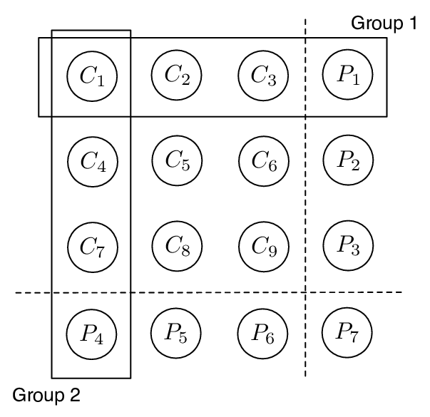
Here, correspond to the content stored at the 16 nodes. In particular, we might interpret that are the systematic bits while are the parity check bits. The code can also be represented by Figure 3. In this case, the parity check equations are equivalent to that the sum of rows and the sum of columns are all zero.
According to (37)-(43), every failed node (either systematic or parity) can be repaired by two different repair groups of size . For instance, if is failed, it can be repaired by repair group or repair group . Notice that the two repair groups are disjoint. Therefore, even if one of the repair groups is not available, there exists an alternative repair group to locally repair the failed node.
It can be verified easily that our code has a minimum distance of 4 and it is a robust locally repairable code. Therefore, any failed node can be repaired by at least repairing group of size in the presence of any extra failure. Also, the original data can be recovered even if there are simultaneous failure. In fact, it is also a robust locally repairable code.
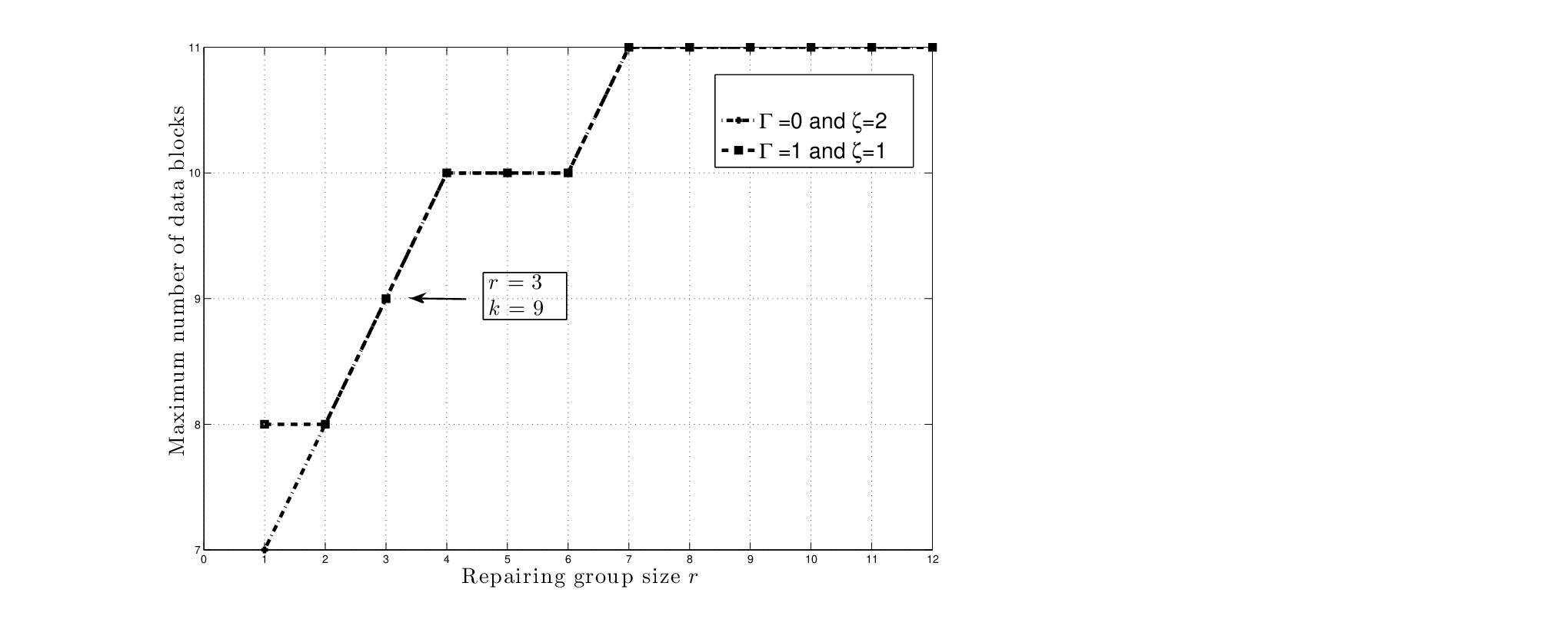
Now, we will use the bound obtained earlier to show that our code is optimal. We have plotted our bound in Figure 4 when and . The horizontal axis is the code locality (i.e., ) and the vertical axis is the dimension of the code (or ). From the figure, when , the dimension of a robust locally repairable code is at most 9. And our constructed code has exactly 9 dimensions. Therefore, our code meets the bound and is optimal. In fact, our bound also indicates that the dimension of a robust locally repairable code is also at most 9. Therefore, our code is in fact an optimal and robust locally repairable code.
Example 2.
Consider a binary linear code of length and dimension defined by the following parity check equations:
| (44) | ||||
| (45) | ||||
| (46) | ||||
| (47) |
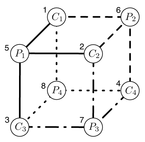
Again, are the information bits while are the parity check bits. The code can be represented by Figure 5. The above parity check equations imply that the sum of any node and its three adjacent nodes in Figure 5 is always equal to zero.
This code has a minimum distance of 4. According to the Equations (44)-(47), for every single node failure, there exists 7 repair groups with size . For example, suppose fails. Then, the repair groups are
Hence, our code is a robust locally repairable code. Furthermore, it can be directly verified that for any distinct ,
| (48) |
and
| (49) |
Therefore, if any one of the surviving nodes is not available, (48) implies that there are still 4 alternative repair groups. This means that our code is also a robust locally repairable code. Similarly, by (49), our code is also a robust locally repairable code.
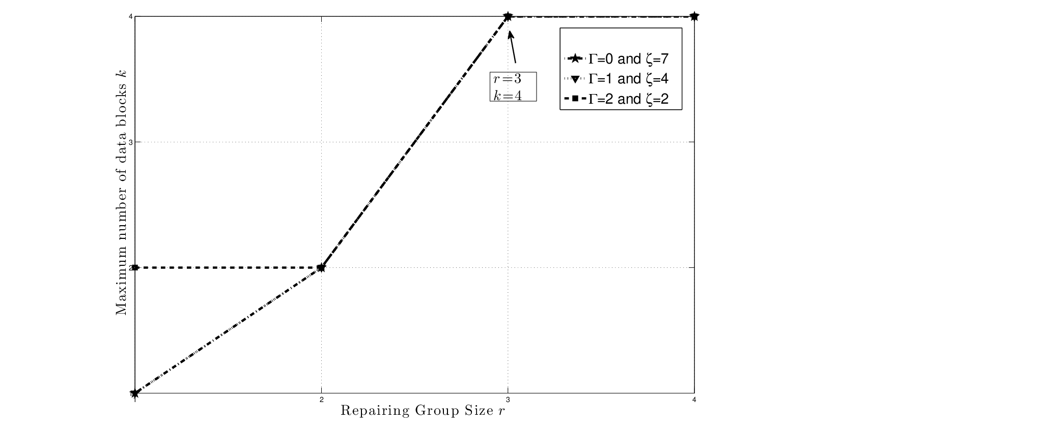
As shown in our bound (see Figure 6), our code has the highest codebook size for the given parameters among all binary , and robust locally repairable codes.
7. Conclusion
In this paper, we characterised the coding scheme for robust locally repairable storage codes. This coding scheme overcomes a significant issue of the locally repairable codes which is their repair inefficiency under the circumstances when there exist extra failures or unavailability in the network. This coding scheme guarantees the local repairability of any failure at the presence of extra failures by constructing multiple local repair groups for each node in the network. In this case, if any of the repair groups is not available during the repair process, there exist alternative groups to locally repair the failed node. We also established a linear programming problem to upper bound the size of these codes. This practical bound can optimise the trade-off between different parameters of the code such as minimum distance, code length, locality, the number of alternative repair groups, and the number of the extra failures. We also provided two optimal robust locally repairable code examples.
The update efficiency of the storage networks was addressed. We characterised an update efficient storage code such that any changes in the stored data will result in a small number of node updates. The necessary conditions for existence of update-efficient storage codes was established.
We also showed how the symmetries in the codes can be exploit to significantly reduce the complexity of the constraints in the linear programming problem and in the necessary conditions.
References
- [1] A. Agarwal, A. Barg, S. Hu, A. Mazumdar and I. Tamo, Combinatorial alphabet-dependent bounds for locally recoverable codes, IEEE Trans. Inf. Theory, 64 (2018), 3481–3492.
- [2] R. Bhagwan, K. Tati, S. S. Y. Cheng and G. Voelker, Total recall: System support for automated availability management, in Proc. NSDI ’04.
- [3] M. Blaum, J. Brady, J. Bruck and J. Menon, Evenodd: An efficient scheme for tolerating double disk failures in raid architectures, IEEE Trans. Inf. Theory, 44 (1995), 192–202.
- [4] M. Blaum, J. Bruck and A. Vardy, MDS array codes with independent parity symbols, IEEE Trans. Inf. Theory, 42 (1996), 529–542.
- [5] M. Blaum, J. L. Hafner and S. Hetzler, Partial-mds codes and their application to raid type of architectures, IEEE Transactions on Information Theory, 59 (2013), 4510–4519.
- [6] W. J. Bolosky, J. R. Douceur, D. ELY and M. Theimer, Feasibility of a serverless distributed file system deployed on an existing set of desktop pcs, in Proc. of Sigmetrics, 2000.
- [7] V. Cadambe and A. Mazumdar, An upper bound on the size of locally recoverable codes, in proc. Int. Symp. Network Coding (NetCod), Calgary, AB, 2013, 1–5.
- [8] V. R. Cadambe and A. Mazumdar, Bounds on the size of locally recoverable codes, IEEE Trans. Inf. Theory, 61 (2015), 5787–5794.
- [9] G. Calis and O. O. Koyluoglu, A general construction for pmds codes, IEEE Communications Letters, 21 (2017), 452–455.
- [10] T. H. Chan, M. A. Tebbi and C. W. Sung, Linear programming bounds for storage codes, in 9th International Conference on Information, Communication, and Signal Processing (ICICS 2013), 2013.
- [11] B. Chen, S.-T. Xia and J. Hao, Locally repairable codes with multiple -localities, in Proc. IEEE Int. Symp. Information Theory (ISIT), Aachen, Germany, 2017, 2038–2042.
- [12] Y. Chen, J. Edler, A. Goldberg, S. S. A. Gottlieb and P. Yianilos, Prototype implementation of archival intermemory, in Proc. of IEEE ICDE, 1996, 485–495.
- [13] A. G. Dimakis, P. B. Godfrey, Y. Wu, M. J. Wainwright and K. Ramchandran, Network coding for distributed storage systems, IEEE Trans. Inf. Theory, 56 (2010), 4539–4551.
- [14] P. Druschel and A. Rowstron, Storage management and caching in past, a large-scale, persistent peer-to-peer storage utility, in Proc. of ACM SOSP, 2001.
- [15] R. Gabrys, E. Yaakobi, M. Blaum and P. H. Siegel, Constructions of partial mds codes over small fields, in 2017 IEEE International Symposium on Information Theory (ISIT), 2017, 1–5.
- [16] P. Gopalan, C. Huang, B. Jenkins and S. Yekhanin, Explicit maximally recoverable codes with locality, IEEE Transactions on Information Theory, 60 (2014), 5245–5256.
- [17] P. Gopalan, C. Huang, H. Simitci and S. Yekhanin, On the locality of codeword symbols, IEEE Trans. Inf. Theory, 58 (2012), 6925–6934.
- [18] C. Huang, M. Chen and J. Li, Pyramid Codes: Flexible Schemes to Trade Space for Access Efficiency in Reliable Data Storage Systems, Technical Report MSR-TR-2007-25, Microsoft Research, 2007.
- [19] S. Kadhe and A. Sprintson, Codes with unequal locality, in Proc. IEEE Int. Symp. Information Theory (ISIT), Barcelona, Spain, 2016, 435–439.
- [20] S. Kadhe and R. Calderbank, Rate optimal binary linear locally repairable codes with small availability, in Proc. IEEE Int. Symp. Information Theory, Aachen, Germany, 2017, 166–170.
- [21] G. M. Kamath, N. Prakash, V. Lalitha and P. V. Kumar, Codes with local regeneration and erasure correction, IEEE Transactions on Information Theory, 60 (2014), 4637–4660.
- [22] O. Khan, R. Burns, J. Park and C. Huang, In search of i/o-optimal recovery from disk failures, in Proceedings of the 3rd USENIX Conference on Hot Topics in Storage and File Systems, HotStorage’11, USENIX Association, Berkeley, CA, USA, 2011, 6–6, URL http://dl.acm.org/citation.cfm?id=2002218.2002224.
- [23] J. Kubiatowicz, D. Bindel, Y. Chen, S. Czerwinski, P. Eaton, D. Geels, R. Gummadi, S. Rhea, H. Weatherspoon, W. Weimer, C. Wells and B. Zhao, Oceanstore: An architecture for global-scale persistent storage, in Proc. 9th Int. Conf. Architectural Support Programm. Lang. Oper. Syst., Boston, MA, 2000, 190–201.
- [24] F. J. Macwilliams and N. J. A. Sloane, The Theory of Error Correcting Codes, North Holland, Amsterdam, 1977.
- [25] U. Martnez-Penas and F. R. Kschischang, Universal and dynamic locally repairable codes with maximal recoverability via sum-rank codes, in 2018 56th Annual Allerton Conference on Communication, Control, and Computing (Allerton), IEEE, 2018, 792–799.
- [26] F. Oggier and A. Datta, Self-repairing homomorphic codes for distributed storage systems, in proc. IEEE INFOCOM, 2011, 1251–1223.
- [27] L. Pamies-Juarez, H. D. Hollmann and F. Oggier, Locally repairable codes with multiple repair alternatives, in proc. IEEE Int. Symp. Information Theory, 2013, 892–896.
- [28] D. S. Papailiopoulos and A. G. Dimakis, Locally repairable codes, in proc. IEEE Int. Symp. Information Theory, Cambridge, MA, 2012, 2771–2775.
- [29] D. Papailiopoulos, J. Luo, A. Dimakis, C. Huang and J. Li, Simple regenerating codes: Network coding for cloud storage, in proc. IEEE INFOCOM, 2012, 2801–2805.
- [30] D. A. Patterson, G. Gibson and R. Katz, A case for redundant arrays of inexpensive disks (raid), Tech. Rep. CSD-87-391, Computer Science Division, Department of Electrical Engineering and Computer Science, University of California, Berkeley, CA 94720, 1987.
- [31] N. Prakash, V. Lalitha and P. Kumar, Codes with locality for two erasures, in Proc. IEEE Int. Symp. Information Theory (ISIT), 2014, 1962–1966.
- [32] A. S. Rawat, O. O. Koyluoglu, N. Silberstein and S. Vishwanath, Optimal locally repairable and secure codes for distributed storage systems, IEEE Transactions on Information Theory, 60 (2014), 212–236.
- [33] A. S. Rawat, A. Mazumdar and S. Vishwanath, On cooperative local repair in distributed storage, in 48th Annual Conference on Information Sciences and Systems (CISS), 2014, 1–5.
- [34] A. S. Rawat, D. S. Papailiopoulos, A. G. Dimakis and S. Vishwanath, Locality and availability in distributed storage, in proc. IEEE Int. Symp. Information Theory, 2014, 681–685.
- [35] S. Rhea, C. Wells, P. Eaton, D. Geels, B. Zhao, H. Weatherspoon and J. Kubiatowicz, Maintenance free global storage in oceanstore, in Poc. of IEEE Internet Computing, 2001, 40–49.
- [36] I. Tamo and A. Barg, Bounds on locally recoverable codes with multiple recovering sets, in proc. IEEE Int. Symp. Information Theory, Honolulu, HI, 2014, 691–695.
- [37] I. Tamo and A. Barg, A family of optimal locally recoverable codes, IEEE Trans. Inf. Theory, 60 (2014), 4661–4676.
- [38] I. Tamo, D. Papailiopoulos and A. Dimakis, Optimal locally repairable codes and connections to matroid theory, in proc. IEEE Int. Symp. Information Theory, Istanbul, 2013, 1814–1818.
- [39] M. A. Tebbi, T. H. Chan and C. Sung, Linear programming bounds for robust locally repairable storage codes, in proc. Information Theory Workshop (ITW), 2014 IEEE, 2014, 50–54.
- [40] A. Wang and Z. Zhang, Repair locality from a combinatorial perspective, in proc. IEEE Int. Symp. Information Theory, 2014, 1972–1976.
- [41] H. Weatherspoon and J. D. Kubiatowicz, Erasure coding vs. replication: A quantitative comparison, in Proc. Int. Workshop Peer-to-Peer Syst., 2002.
- [42] S. B. Wicker, Error Control Systems for Digital Communication and Storage, Prentice Hall, Englewood Cliffs, NJ, 1995.
- [43] A. Zeh and E. Yaakobi, Bounds and constructions of codes with multiple localities, in Proc. IEEE Int. Symp. Information Theory (ISIT), Barcelona, Spain, 2016, 640–644.
Received xxxx 20xx; revised xxxx 20xx.