Automatic Salient Object Detection for Panoramic Images Using Region Growing and Fixation Prediction Model
Abstract
Almost all previous works on saliency detection have been dedicated to conventional images, however, with the outbreak of panoramic images due to the rapid development of VR or AR technology, it is becoming more challenging, meanwhile valuable for extracting salient contents in panoramic images.
In this paper, we propose a novel bottom-up salient object detection framework for panoramic images. First, we employ a spatial density estimation method to roughly extract object proposal regions, with the help of region growing algorithm. Meanwhile, an eye fixation model is utilized to predict visually attractive parts in the image from the perspective of the human visual search mechanism. Then, the previous results are combined by the maxima normalization to get the coarse saliency map. Finally, a refinement step based on geodesic distance is utilized for post-processing to derive the final saliency map.
To fairly evaluate the performance of the proposed approach, we propose a high-quality dataset of panoramic images (SalPan). Extensive evaluations demonstrate the effectiveness of our proposed method on panoramic images and the superiority of the proposed method against other methods.
Index Terms:
Saliency detection, eye fixation, region growing, panoramic images.I Introduction
An inherent and powerful ability of human eyes is to quickly capture the most conspicuous regions from a scene, and passes them to high-level visual cortexes. The neurobiological attention mechanism reduces the complexity of visual analysis and thus makes human visual system considerably efficient in complex scenes.
Early work [17] on computing saliency aimed to model and predict human gaze on images. Recently the field has expanded to include the segmentation of entire salient regions or objects [1]. Most works [22, 56, 57, 55, 60, 54, DBLP:journals/corr/abs-1711-00322] extract salient regions which exhibit highly distinctive features compared to their surrounding regions, based on the concept of center-surround contrast. Moreover, additional prior knowledge for spatial layout of foreground objects and background can be also used [46, 61, 33, 7]. These assumptions have been successfully employed to improve the performance of saliency detection for conventional images with common aspect ratios. However, existing bottom-up methods [32] show somewhat poor performance for complex situations. With the development of neural networks, some algorithms [50] adopt deep learning based methods to deal with this problem. This trend is analogous to the biological evolution process, which can be regarded as evolutionary theory of saliency detection (shown in the right of Fig.1).

Recently, panoramic images, which yield wide fields of view, become popular in all kinds of media contents and draw much attention in many practical applications. However, to accurately calculate visual saliency of panoramic images, both traditional methods and deep learning based methods proposed in recent years would fail in some cases of panoramic images, where complex background is present (shown in the left of Fig.1). Thus we propose an effective saliency detection framework for panoramic images.
In this work, we propose an automatic salient object detection framework for panoramic images using a dual-stage region growing and fixation prediction model. Panoramic images exert several distinct characteristics compared to conventional images. We find that spatial density patterns is useful for images with high resolutions. Therefore, we first employ a spatial density pattern detection method for the panoramic image to roughly extract the proposal regions, and use a dual-stage region growing process to get the proposed regions. Meanwhile, the eye fixation model is deployed in the framework to locate the focus of visual attention in images, which is inspired by the mechanisms of the human vision system. Then, the previous saliency information is combined by the maxima normalization to get the coarse saliency map. Finally, a geodesic refinement is employed to derive the final saliency map.
The main contributions of this paper are listed as follows:
1. A new automatic salient object detection framework is proposed for panoramic images, which combines the usage of region growing and eye fixation model. Density map is first introduced in our work as a feature representation for saliency calculation.
2. To fairly evaluate the performance of the proposed method, we build a new high-quality panoramic dataset (SalPan) with an accurate ground truth annotation method which can eliminate the ambiguous of salient objects. This SalPan dataset will be released publicly after publication.
3. Compared with both conventional algorithms and deep learning based algorithms, the proposed method achieves the state-of-the-art performance on SalPan dataset and other large-scale salient object detection datasets including the recent ECSSD [36], DUT-OMRON [51] and SED [4]. In addition, the proposed algorithm is fast on both modern CPUs and GPUs.
4. The proposed framework can also be tailored for small target detection.
To our thoughts, this research may help to exploit the perception characteristics of the human visual system for large-scale visual contents over a wide field of view.
The rest of this paper is organized as follows. Section 2 briefly reviews related work. Sections 3 explains the proposed framework. Section 4 presents the experimental results. Section 5 discusses some practical guidelines. Section 6 concludes this paper.
II Related Works
In this section, we have a brief review of classical eye fixation models, traditional saliency algorithms and deep learning based saliency detection methods.
II-A Eye Fixation Model
The first models for saliency prediction were biologically inspired and based on a bottom-up computational model that extracted low-level visual features such as intensity, color, orientation, texture and motion at multiple scales. Itti et al. [17] proposed a model that combines multiscale low-level features to create a saliency map. Harel et al. [6] presented a graph-based alternative that starts from low-level feature maps and creates Markov chains over various image maps, treating the equilibrium distribution over map locations as activation and saliency values. Since the eye fixation model can mimic the process of the human visual system, thus, we embed the fixation prediction model into our framework.
II-B Traditional Saliency Algorithm
Saliency detection for conventional images could be implemented based on either top-down or bottom-up models. Top-down models [31, 11, 10, 49, chen2017m] required high level interpretation usually provided by training sets in supervised learning. Contextual saliency was formulated according to the study of visual cognition: global scene context of an image was highly associated with a salient object [31]. The most distinct features were selected by information theory based methods [10]. Salient objects were detected by joint learning of a dictionary for object features and conditional random field classifiers for object categorization [49]. While these supervised approaches can effectively detect salient regions and perform overall better than bottom-up approaches, it is still expensive to perform the training process, especially data collection.
In contrary, bottom-up models [32, 37, 58, 23, 59, crm2016spl, crm2018tip] did not require prior knowledge such as object categories, but obtained saliency maps by using low level features based on the center-surround contrast. They computed feature distinctness of a target region, e.g., pixel, patch or superpixel, compared to its surrounding regions locally or globally. For example, feature difference was computed across multiple scales, where a fine scale feature map represented the feature of each pixel while a coarse scale feature map described the features of surrounding regions [17]. Also, to compute center-surround feature contrast, spatially neighboring pixels were assigned different weights [13], or random walk on a graph was used [19].
Bottom-up based approaches did not need data collection and training process, consequently requiring little prior knowledge. These advantages make bottom-up approaches more efficient and easy to implement in a wide range of real computer vision applications. A complete survey of these methods is beyond the scope of this paper and we refer the readers to a recent survey paper [5] for details. In this paper, we focus on the bottom-up approach.
II-C Deep Learning based Saliency Detection Method
With the performance of deep convolutional neural achieving near human-level performance in image classification and recognition task. Many algorithms adopt deep learning based methods [50, 43, 21, 12, 44, 20, 53]. Instead of constructing hand-craft features, this kind of top-down methods have achieved state-of-the-art performance on many saliency detection datasets. However, deep learning based algorithms exist the following limitations: 1) need a large number of annotated data for training. (2) very time-consuming in the learning process even with GPU of high computation ability. (3) training instances are not uniformly sampled. (4) sensitive to noise in training samples and image resolution.
Bottom-up based approaches do not need data collection and training process, consequently requiring little prior knowledge. These make bottom-up approaches more suitable for real-time applications. Meanwhile, bottom-up methods are not sensitive to image scale, capacity and type. These advantages make bottom-up approaches more efficient and easy to panoramic saliency detection. In this paper, we focus on the bottom-up approach.
III The Proposed Framework
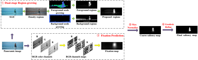
Here we describe the proposed framework in four main steps. First, we employ a dual-stage region-growing algorithm for salient regions proposal. Second, an eye fixation prediction model is used to find visually attractive locations in the image, which is then combined with proposal regions in the previous step to form a reliable saliency map. Third, a maxima normalization is utilized to optimize the previous saliency information. Fourth, the final saliency map is obtained after a refinement step based on geodesic distance. The main framework is depicted in Fig. 2s.
III-A A Dual-stage Region-growing Based Detection
In this section, we first use the efficient Simple Linear Iterative Clustering (SLIC) algorithm [28] to segment the image into smaller superpixel elements in order to capture the essential local structural information of the image. Then , we roughly extract regions that have significant and different densities compared with its neighbors. After obtaining the proposal regions, we use a dual-stage seed estimation and growing to improve previous map. One is the foreground seeds based ranking process, the other is the background seeds based ranking process. Finally, we merge the two detection results to get the proposed salient regions.
III-A1 Density Map
The notion of density comes from fractal theory. Density measures locally the variation of a quantity over a number of scales. It has been used before for texture classification [30]. The idea is that at small scales naturally occurring objects (here the texture) change over scale in a way, that can be modeled as an exponential function of the scale. Thus the exponent of the function is a good statistical descriptor of the object which is invariant to a wide range of spatial transformations. In this work we focus on the density variation property of the density map.
Let be a grayscale image and let be a measure on . For our purposes we choose to be the sum of image intensities in a disk of radius around point , i.e. . We use the power law to express as a function of :
| (1) |
| (2) |
| (3) |
We define the exponent , also known as Holder exponent, to be the local density function of image at point . Intuitively, it measures the degree of regularity of intensity variation in a local neighbourhood around point .
The density map values are the same within regions of different intensity as well as within regions of smoothly varying intensity. In essence, the density map preserves important textural features by responding to abrupt intensity discontinuities and avoiding smoothly varying regions. In our work, the obtained density map is utilized as a feature map for coarse salient region proposals. We adopt the region-based contrast method for this purpose. GrabCut [35]is used to segment the image into a number of regions, then saliency computation is performed on these regions. The saliency value of each regions is derived as follows:
| (4) |
where is the weight of region and is the density distance metric between the two regions.
| (5) |
where is the probability of the -th density among all densities in the -th region , .
In the end, the map is binarized to obtain a mask, which could be treated as object region proposals. The mask map is denoted .
III-A2 Foreground Seeds based Region Growing
We denote the map generated by previous section, , which indicates proposed density regions.
Unlike previous works[24, 48] that treat some regions as certain seeds, we provide a more flexible scheme for seeds estimation. We define two types of seed elements: strong seeds and weak seeds. Strong seeds have high probability of belonging to foreground/background while weak seeds have relatively low probability of belonging to foreground/background. For foreground seeds, the two types of seeds are selected by:
| (6) |
| (7) | ||||
where denotes the set of strong seeds and weak seeds, represent th superpixel. mean(.) is the averaging function. It is obvious from formula (6)(7) that elements of higher degree of surroundedness are more likely to be chosen as strong foreground seeds, which is consistent with intuition.
For saliency calculation based on given seeds, a ranking method in [52] that exploits the intrinsic manifold structure of data for graph labelling is utilized. The ranking method is to rank the relevance of every element to the given set of seeds. We construct a graph that can represent an whole image as in work [48], where each node is a superpixel generated by SLIC.
The ranking procedure is as follows: Given a graph ,where the nodes are and the edges are weighted by an affinity matrix . The degree matrix is defined by , where . The ranking function is given by:
| (8) |
The is the resulting vector which stores the ranking results of each element. The is a vector indicating the seed queries.
In this work, the weight between two nodes is defined by:
| (9) |
where and denote the mean of the superpixels corresponding to two nodes in the CIE LAB color space, and is a constant that controls the strength of the weight.
Different from [48] that define if is a query and otherwise, we define as the strength of the query extra. That is, if is a strong query, and if is a weak query, and otherwise.
III-A3 Background Seeds based Region Growing
Complementary to foreground seeds estimation and growing, background seeds estimation and growing aims to extract regions that are different from background in feature distribution. We first select a set of background seeds and then calculate saliency of every image element according to its relevance to these seeds. We divide the elements on image border into two categories(strong seeds and weak seeds) as in foreground situation. We denote the average value of all border elements as . The euclidean distance between each feature vector and the average feature vector is computed by , the average of is denoted by . The background seeds are estimated by:
| (10) |
| (11) |
where denotes strong background seeds, denotes weak background seeds.
Similar to foreground situation, the value of indication vector for background seeds is if belongs to , if belongs to and 0 otherwise. Relevance of each element to background seeds is computed by formula (8). Elements in resulting vector indicates the relevance of a node to the background queries, and its complement is the saliency measure.The saliency map using these background seeds can be written as:
| (12) |
The background saliency map and foreground saliency map is combined by multiplication to form a coarse saliency map, as shown in the end of stage 1 in Fig.2.
III-B Fixation prediction
Whether a location is salient or not largely depends on how much it attracts human attention. A large number of recent works on eye fixation prediction have revealed more or less the nature of this issue. Eye fixation prediction models simulate the mechanisms of the human visual system, and thus can predict the probability of a location to attract human attention. So in this section, we use eye fixation model to help us ensure which region has more power to grab human attention.
Panoramic images are often with wide fields of view, and consequently are computationally more expensive compared with conventional images. Algorithms based on color contrast, local information are not suitable for being a preprocessing step for panoramic images, for these algorithms are time-consuming and would spend a lot of computational resources. Thus we are seeking a more efficient method to help us to rapidly scan the image and roughly locate where attract human attention. Obviously Fixation prediction models in frequency domain fit this demand, for these models are computationally efficient and easy to implement.
The signature model approximately isolate the spatial support of foreground by taking the sign of the mixture signal x in the transformed domain and then transform it back to spatial domain, i.e., by computing the reconstructed image . stands for DCT transform of . The image signature is defined as
| (13) |
And the saliency map is formed by smoothing the squared reconstructed image defined above
| (14) |
where is a Gaussian kernel.
The image signature is a simple yet powerful descriptor of natural scenes, and it can be used to approximate the spatial location of a sparse foreground hidden in a spectrally sparse background. Compared with other eye fixation models, image signature has a more efficient implementation, which runs faster than all other competitors.
To combine the proposed salient regions in previous section with saliency map produced by image signature, we assign the saliency value of the proposed salient regions by averaging the saliency values of all its pixels inside. For convenience we denote the resulted saliency map as . That is, for a proposed region , its saliency value is defined as
| (15) |
where denote the number of pixels in the th region.
As shown in Fig.3, fixation prediction model reliably locate visually attractive positions, while density detection pops out a number of proposal regions. One is for reliable but fuzzy locating saliency, while the other is for rich pop-out object proposals. These two step are therefore complementary.

III-C Maxima Normalization
Fusing saliency detection results of multiple models has been recognized as a challenging task since the candidate models are usually developed based on different cues or assumptions. Fortunately, in our case, the integration problem is relatively easier since we only consider the outputs from two pathways. Since there is no prior knowledge or other top-down guidance can be used, it is safer to utilize the map statistics to determine the importance of each pathway. Intuitively in the final integration stage, we combine the results from two pathways by summing them after Maxima Normalization (MN) (Algorithm 1).
Input: Previous map , thresh of local maxima ;
Output: Normalized Saliency Map ;
The Maxima Normalization operator (.) was originally proposed for the integration of conspicuous maps from multiple feature channels [17], which has been demonstrated very effective and has a very convincing psychological explanation.
III-D Geodesic refinement
The final step of our proposed approach is refinement with geodesic distance [39]. The motivation underlying this operation is based on thought that determining saliency of an element as weighted sum of saliency of its surrounding elements, where weights are corresponding to Euclidean distance, has a limited performance in uniformly highlighting salient object. We tend to find a solution that could enhance regions of salient object more uniformly. From recent works [61], we found the weights may be sensitive to geodesic distance.
The input image is first segmented into a number of superpixels based on linear spectral clustering method [13] and the posterior probability of each superpixel is calculated by maxima normalization operation of all its pixels inside. For th superpixel, if its posterior probability is labeled as , thus the saliency value of the th superpixel is refined by geodesic distance as follows:
| (16) |
where is the total number of superpixels, and will be a weight based on geodesic distance [61] between th superpixel and th superpixel.
First, an undirected weight graph has been constructed connecting all adjacent superpixels and assigning their weight as the Euclidean distance between their saliency values which are derived in the previous section. Then the geodesic distance between two superpixels can be defined as accumulated edge weights along their shortest path on the graph:
| (17) |
In this way we can get geodesic distance between any two superpixels in the image. Then the weight is defined as
| (18) |
where is the deviation for all values. From formula (6) we can easily conclude that when and are in flat region, saliency value of would have a higher contribution to saliency value of , and when and are in different regions between which a steep slope is existed, saliency value of tends to have a less contribution to saliency value of .
Since an object often contains some homogenous parts, the initial saliency value of a superpixel could be spread to the other connected homogenous parts, indicating the propagation may be achieved through connectivity. This can also be observed in the background where image background can be divided into large homogenous regions. Noting that the coarse saliency could render more saliency to the target object while less to the background (Fig.2). Hence, low saliency in background part could be spread over the entire background region after propagation. Eventually, the background could be suppressed to very low saliency values.
IV Experiments
To fairly evaluate the performance of the proposed framework, we build a new dataset of panoramic landscape images (SalPan), and evaluate the performance of the proposed saliency detection algorithm compared with 12 state-of-the-arts methods. More experimental analysis on the effectiveness of our method are given as follows.
IV-A Datasets
We collect a new panoramic dataset SalPan composed of 123 panoramic images. In general, saliency may be ambiguous in images with highly complex scenes and wide fields of view, thus we propose an accurate ground truth annotation method to eliminate the ambiguous.
To build a ground-truth for SalPan dataset we first conducted a comprehensive user study. To identify where participants were looking while watching the films, we monitor their eye movements using a Gazepoint GP3 Eye Tracker. Image presentation was controlled using the Gazepoint Analysis Standard software. For the purpose of the study we recruited 10 participants (5 males, 5 females). Ages ranged from 20 to 57 with the mean age of 25. All the participants had normal or corrected-to-normal vision and were naive to the underlying purposes of the experiment. Then, we record the tracking path and allocate values to each eye movement location according to the times of visual attention. Finally, we pick up those values above the average and label the ground truth with complete objects corresponding attention points.
Meanwhile, we make the image acquisition and image annotation independent to each other, we can avoid dataset design bias, namely a specific type of bias that is caused by experimenters’ unnatural selection of dataset images. After picking up the salient regions, we adhere to the following rules to build the ground truth:
disconnected regions of the same objects are labeled separately;
solid regions are used to approximate hollow objects, such as bike wheels.
The process of labeling the ground truth is shown in Fig. 4.

IV-B Evaluation indicators
Experimental evaluations are based on standard measurements including precision-recall curve, precision value, recall value, AUC value, MAE (Mean Absolute Error) value, time-consuming with coding type and F-measure.
Besides, We also adopt a new structural similarity measure known as Structure-measure (S-measure, proposed in ICCV17) [8] which simultaneously evaluates region-aware and object aware structural similarities between a saliency map and a ground-truth map.
The precision is defined as:
| (19) |
where indicates the set that binarized from a saliency map using threshold . is the set of pixels belonging to groundtruth salient object.
The recall is defined as:
| (20) |
The precision-recall curve is plotted by connecting the P-R scores for all thresholds.
The MAE is formulated as:
| (21) |
where is the number of the testing images, is the area of the ground truth of an image , is the area of the result of an image .
The F-measure is formulated as:
| (22) |
where is set to 0.3 as did in many literatures.
The S-measure is formulated as:
| (23) |
where and are region-aware and object-aware structural similarity evaluation value, respectively.

IV-C Ablation study
We first validate the effectiveness of each step in our method: foreground seeds based region-growing (R-F), background seeds based region-growing (R-B),a dual-stage region-growing based detection (R-M), fixation prediction saliency detection (FP), maxima normalization fusion (MN) and geodesic refinement (GR). Table.I shows the validation results on SalPan dataset. We can clear see the accumulated processing gains after each step, and the final saliency results shows a good performance. After all, it proves that each steps in our algorithm is effective for generating the final saliency maps.
| * | Step 1 | Step 2 | Step 3 | Step 4 | ||
|---|---|---|---|---|---|---|
| R-F | R-B | R-M | FP | MN | GR | |
| MAE | .291 | .287 | .271 | .311 | .256 | .231 |
| F-m | .689 | .694 | .715 | .646 | .734 | .767 |
| S-m | .727 | .731 | .737 | .694 | .752 | .783 |
Fig. 8 show two group visual process of each steps of the proposed method. Step 1: Dual-stage Region growing. Step 2: Fixation Prediction. Step 3: Max Normalization. Step 4: Geodesic Refinement. From the process shown in the figure, we can see the details of our framework and how each step contribute to the final result.
| * | MAE Value | AUC Value | Precision Value | Recall Value | F-measure | S-measure | Time(s) | Code Type |
| FT | 0.3868 | 0.5072 | 0.4942 | 0.4286 | 0.4643 | 0.5580 | 0.593 | C |
| NPS | 0.3613 | 0.4213 | 0.3973 | 0.4195 | 0.4053 | 0.4722 | 2.397 | M C |
| CB | 0.4238 | 0.6515 | 0.5112 | 0.5398 | 0.5125 | 0.6095 | 4.196 | M C |
| SPL | 0.3125 | 0.4517 | 0.4324 | 0.3861 | 0.4060 | 0.5156 | 1.926 | M C |
| MSS | 0.4627 | 0.5221 | 0.5185 | 0.4234 | 0.4621 | 0.5912 | 3.893 | M C |
| BSCA | 0.4137 | 0.5115 | 0.4716 | 0.4067 | 0.4360 | 0.6079 | 1.876 | M C |
| LPS | 0.3697 | 0.5184 | 0.4867 | 0.4794 | 0.4810 | 0.5812 | 2.193 | M C |
| HS | 0.4090 | 0.6816 | 0.5212 | 0.5692 | 0.5597 | 0.6395 | 2.896 | M C |
| DRFI | 0.3592 | 0.7021 | 0.6319 | 0.5710 | 0.6072 | 0.6402 | 1.903 | M C |
| KSR | 0.3222 | 0.4608 | 0.4345 | 0.3507 | 0.4056 | 0.5397 | 2.537 | M C |
| WSS | 0.3090 | 0.6507 | 0.6687 | 0.6380 | 0.6546 | 0.7579 | 2.751 | M C |
| Amulet | 0.3179 | 0.6321 | 0.5962 | 0.6119 | 0.6069 | 0.7121 | 3.216 | M C |
| OURS | 0.2744 | 0.8024 | 0.7614 | 0.6753 | 0.7142 | 0.7832 | 1.075 | M C |
IV-D Comparison
To illustrate the effectiveness of our algorithm, we compare our proposed methods with other 12 state-of-the-art ones including 9 conventional algorithms (FT [1], NPS [15], CB [18], SPL [26], MSS [41], BSCA [32], LPS [23], HS [37], DRFI [42]) and 3 deep learning based algorithms (KSR [45], WSS [43] and Amulet [50]). We use the codes provided by the authors to reproduce their experiments. For all the compared methods, we use the default settings suggested by the authors.
Fig. 5 compares the PR curves, where we see that the proposed algorithm achieves a much higher performance than that of the existing methods.
As observed in Fig. 5, we see that the proposed algorithm has a higher F-measure score and S-measure score than any other competitors.
We measure the MAE value, precision value, recall value, AUC value, F-measure value and S-measure value using a resulting saliency map against the ground truth saliency map, which are shown in Table.II. We have seen that the proposed algorithm also achieves the best performance and outperforms all other compared methods.
We also compare the average execution times of the proposed algorithm and the other methods in Table II. Most of the methods including the proposed one are implemented using MATLAB and executed on an Intel i7 3.4 GHz CPU with 16 GB RAM. Results show that most of the existing methods consume more time than the proposed algorithm.
In summary, from the comparison, we can conclude that our saliency results are more robustness and efficient on SalPan dataset. Besides, the visual comparisons shown in Fig. 6 clearly demonstrate the advantages of the proposed method. We can see that our method can extract both single and multiple salient objects precisely. In contrast, the compared methods may fail in some situations.
V Discussion
Comparison in conventional datasets. To further fairly verify the performance of the proposed method. We also compare our algorithm with other 12 state-of-the-art ones on 3 public saliency detection datasets, including ECSSD [36], DUT-OMRON [51] and SED [4].
Visual comparisons of salient region detection results are shown in Fig. 9. GT represents Ground Truth. The proposed method also shows good results on conventional datasets, which is in consistent with panoramic datasets.

Small target detection. It is very interesting to find that the proposed automatic salient object detection algorithm for panoramic images using region growing and eye fixation model is also valid for small target detection. We present a part of our experimental results on the small target dataset [27]. Small target detection plays an important role in many computer vision tasks, including early alarming system, remote sensing and visual tracking. The experimental results by applying the proposed algorithm to small target detections in Fig. 5, respectively, which support our claim.
The underlying reason why the proposed algorithm can be applied in small target detection and conventional images’ saliency detection is that: the panoramic images also contain small objects and big objects, so, the image with the small target and conventional image can be seen as the part of its.
Therefore, we claim that the proposed automatic salient object detection algorithm is not only confined to panoramic images but also conventional images and the images with small target.


Limitation of the proposed method. Since our method is bottom-up methods, which is not sensitive to the edge information. It sometimes fails to render complete boundary information in very complex scenarios. We hope to mitigate this issue by exploring various forms of edge processing methods in the future.
VI Conclusion
In this paper, we proposed a novel bottom-up saliency detection framework for panoramic images. We first employed a spatial density pattern detection method based on dual-stage region growing for the panoramic image to obtain the proposal regions. Meanwhile, the fixation prediction model was embedded into the framework to locate the focus of attention in images. Then, the previous saliency information was combined by the maxima normalization to obtain the coarse saliency map. Finally, a geodesic refinement was utilized to get the final saliency map.
Experimental results demonstrated that the proposed saliency detection algorithm provided reliable saliency maps for panoramic images, and outperformed the recent state-of-the-art saliency detection methods qualitatively and quantitatively. Moreover, the proposed algorithm also yielded competitive performance to the existing saliency detection methods on the conventional image dataset with common aspect ratios.
Our future research efforts include the extension of SalPan dataset and the evaluation of algorithm performance on more diverse panoramic scenes. To encourage future work, we will make the source codes, experiment data, SalPan dataset for the research community public.
Acknowledgment
This work was supported by the grant of National Natural Science Foundation of China(No.U1611461), the grant of Science and Technology Planning Project of Guangdong Province, China(No.2014B090910001) and the grant of Shenzhen PeacockPlan(No.20130408-183003656).
References
- [1] R. Achanta, S. Hemami, F. Estrada, and S. Susstrunk. Frequency-tuned salient region detection. In Computer Vision and Pattern Recognition, 2009. CVPR 2009. IEEE Conference on, pages 1597–1604, 2009.
- [2] B. Alexe, T. Deselaers, and V. Ferrari. Measuring the objectness of image windows. IEEE Transactions on Pattern Analysis and Machine Intelligence, 34(11):2189, 2012.
- [3] A. Borji. Boosting bottom-up and top-down visual features for saliency estimation. In Computer Vision and Pattern Recognition, pages 438–445, 2012.
- [4] A. Borji. What is a salient object? a dataset and a baseline model for salient object detection. IEEE Transactions on Image Processing, 24(2):742, 2015.
- [5] A. Borji, M. M. Cheng, H. Jiang, and J. Li. Salient object detection: A survey. Eprint Arxiv, 16(7):3118, 2014.
- [6] M. Cerf, J. Harel, W. Einh?user, and C. Koch. Predicting human gaze using low-level saliency combined with face detection. In International Conference on Neural Information Processing Systems, pages 241–248, 2008.
- [7] M. M. Cheng, J. Warrell, W. Y. Lin, S. Zheng, V. Vineet, and N. Crook. Efficient salient region detection with soft image abstraction. In IEEE International Conference on Computer Vision, pages 1529–1536, 2013.
- [8] D.-P. Fan, M.-M. Cheng, Y. Liu, T. Li, and A. Borji. Structure-measure: A new way to evaluate foreground maps. In Proceedings of the IEEE Conference on Computer Vision and Pattern Recognition, pages 4548–4557, 2017.
- [9] S. Frintrop. General object tracking with a component-based target descriptor. In IEEE International Conference on Robotics and Automation, pages 4531–4536, 2010.
- [10] D. Gao, S. Han, and N. Vasconcelos. Discriminant saliency, the detection of suspicious coincidences, and applications to visual recognition. IEEE Transactions on Pattern Analysis and Machine Intelligence, 31(6):989–1005, 2009.
- [11] D. Gao and N. Vasconcelos. Discriminant saliency for visual recognition from cluttered scenes. Advances in Neural Information Processing Systems, 17:481–488, 2004.
- [12] K. He, X. Zhang, S. Ren, and J. Sun. Delving deep into rectifiers: Surpassing human-level performance on imagenet classification. In IEEE International Conference on Computer Vision, pages 1026–1034, 2016.
- [13] A. Hornung, Y. Pritch, P. Krahenbuhl, and F. Perazzi. Saliency filters: Contrast based filtering for salient region detection. In IEEE Conference on Computer Vision and Pattern Recognition, pages 733–740, 2012.
- [14] X. Hou and L. Zhang. Saliency detection: A spectral residual approach. In IEEE Conference on Computer Vision and Pattern Recognition, pages 1–8, 2007.
- [15] X. Hou and L. Zhang. Dynamic visual attention: Searching for coding length increments. In Conference on Neural Information Processing Systems, Vancouver, British Columbia, Canada, December, pages 681–688, 2009.
- [16] L. Itti. Automatic foveation for video compression using a neurobiological model of visual attention. IEEE Transactions on Image Processing A Publication of the IEEE Signal Processing Society, 13(10):1304, 2004.
- [17] L. Itti, C. Koch, and E. Niebur. A model of saliency-based visual attention for rapid scene analysis. IEEE Transactions on Pattern Analysis and Machine Intelligence, 20(11):1254–1259, 1998.
- [18] H. Jiang, J. Wang, Z. Yuan, T. Liu, N. Zheng, and S. Li. Automatic salient object segmentation based on context and shape prior. In British Machine Vision Conference, 2011.
- [19] J. S. Kim, J. Y. Sim, and C. S. Kim. Multiscale saliency detection using random walk with restart. IEEE Transactions on Circuits and Systems for Video Technology, 24(2):198–210, 2014.
- [20] G. Li and Y. Yu. Visual saliency based on multiscale deep features. In Computer Vision and Pattern Recognition, pages 5455–5463, 2015.
- [21] G. Li and Y. Yu. Deep contrast learning for salient object detection. In Computer Vision and Pattern Recognition, pages 478–487, 2016.
- [22] G. Li and C. Zhu. A three-pathway psychobiological framework of salient object detection using stereoscopic technology. In 2017 ICCVW, pages 3008–3014, Oct 2017.
- [23] H. Li, H. Lu, Z. Lin, X. Shen, and B. Price. Inner and Inter Label Propagation: Salient Object Detection in the Wild. New Park Pub.,, 2015.
- [24] X. Li, H. Lu, L. Zhang, R. Xiang, and M. H. Yang. Saliency detection via dense and sparse reconstruction. In IEEE International Conference on Computer Vision, pages 2976–2983, 2013.
- [25] C. C. Lin, S. U. Pankanti, K. N. Ramamurthy, and A. Y. Aravkin. Adaptive as-natural-as-possible image stitching. In IEEE Conference on Computer Vision and Pattern Recognition, pages 1155–1163, 2015.
- [26] Z. Liu, X. Zhang, S. Luo, and O. L. Meur. Superpixel-based spatiotemporal saliency detection. IEEE Transactions on Circuits and Systems for Video Technology, 24(9):1522–1540, 2014.
- [27] J. Lou, W. Zhu, H. Wang, and M. Ren. Small target detection combining regional stability and saliency in a color image. Multimedia Tools and Applications, 76(13):14781–14798, 2017.
- [28] A. Lucchi, K. Smith, R. Achanta, G. Knott, and P. Fua. Supervoxel-based segmentation of mitochondria in em image stacks with learned shape features. IEEE Transactions on Medical Imaging, 31(2):474–486, 2012.
- [29] Y. Luo, J. Yuan, P. Xue, and Q. Tian. Saliency density maximization for efficient visual objects discovery. IEEE Transactions on Circuits and Systems for Video Technology, 21(12):1822–1834, 2011.
- [30] D. R. G. J. Miller. Viewpoint invariant texture description using fractal analysis. International Journal of Computer Vision, 83(1):85–100, 2009.
- [31] A. Oliva, A. Torralba, M. S. Castelhano, and J. M. Henderson. Top-down control of visual attention in object detection. In International Conference on Image Processing, 2003. ICIP 2003. Proceedings, pages I–253–6 vol.1, 2003.
- [32] Y. Qin, H. Lu, Y. Xu, and H. Wang. Saliency detection via cellular automata. In Computer Vision and Pattern Recognition, pages 110–119, 2015.
- [33] M. Ran, A. Tal, and L. Zelnikmanor. What makes a patch distinct? In IEEE Conference on Computer Vision and Pattern Recognition, pages 1139–1146, 2013.
- [34] R. Rosenholtz, A. Dorai, and R. Freeman. Do predictions of visual perception aid design? Acm Transactions on Applied Perception, 8(2):1–20, 2011.
- [35] C. Rother, V. Kolmogorov, and A. Blake. ”grabcut”: interactive foreground extraction using iterated graph cuts. In ACM SIGGRAPH, pages 309–314, 2004.
- [36] J. Shi, Q. Yan, X. Li, and J. Jia. Hierarchical image saliency detection on extended cssd. IEEE Transactions on Pattern Analysis and Machine Intelligence, 38(4):717–729, 2016.
- [37] J. Shi, Q. Yan, X. Li, and J. Jia. Hierarchical image saliency detection on extended cssd. IEEE Transactions on Pattern Analysis and Machine Intelligence, 38(4):717, 2016.
- [38] C. Siagian and L. Itti. Biologically inspired mobile robot vision localization. IEEE Transactions on Robotics, 25(4):861–873, 2009.
- [39] J. B. Tenenbaum, S. V. De, and J. C. Langford. A global geometric framework for nonlinear dimensionality reduction. Science, 290(5500):2319, 2000.
- [40] J. Tilke, K. Ehinger, F. Durand, and A. Torralba. Learning to predict where humans look. 30(2):2106–2113, 2009.
- [41] N. Tong, H. Lu, L. Zhang, and R. Xiang. Saliency detection with multi-scale superpixels. IEEE Signal Processing Letters, 21(9):1035–1039, 2014.
- [42] J. Wang, H. Jiang, Z. Yuan, M.-M. Cheng, X. Hu, and N. Zheng. Salient object detection: A discriminative regional feature integration approach. International Journal of Computer Vision, 123(2):251–268, Jun 2017.
- [43] L. Wang, H. Lu, Y. Wang, M. Feng, D. Wang, B. Yin, and X. Ruan. Learning to detect salient objects with image-level supervision. In Proceedings of the IEEE Conference on Computer Vision and Pattern Recognition, pages 136–145, 2017.
- [44] L. Wang, L. Wang, H. Lu, P. Zhang, and R. Xiang. Saliency detection with recurrent fully convolutional networks. In European Conference on Computer Vision, pages 825–841, 2016.
- [45] T. Wang, L. Zhang, H. Lu, C. Sun, and J. Qi. Kernelized subspace ranking for saliency detection. In European Conference on Computer Vision, pages 450–466. Springer, 2016.
- [46] Y. Wei, F. Wen, W. Zhu, and J. Sun. Geodesic Saliency Using Background Priors. Springer Berlin Heidelberg, 2012.
- [47] C. Yang, L. Zhang, and H. Lu. Graph-regularized saliency detection with convex-hull-based center prior. IEEE Signal Processing Letters, 20(7):637–640, 2013.
- [48] C. Yang, L. Zhang, H. Lu, X. Ruan, and M. H. Yang. Saliency detection via graph-based manifold ranking. In IEEE Conference on Computer Vision and Pattern Recognition, pages 3166–3173, 2013.
- [49] J. Yang. Top-down visual saliency via joint crf and dictionary learning. In Computer Vision and Pattern Recognition, pages 2296–2303, 2012.
- [50] P. Zhang, D. Wang, H. Lu, H. Wang, and X. Ruan. Amulet: Aggregating multi-level convolutional features for salient object detection. In Proceedings of the IEEE Conference on Computer Vision and Pattern Recognition, pages 202–211, 2017.
- [51] R. Zhao, W. Ouyang, H. Li, and X. Wang. Saliency detection by multi-context deep learning. In Computer Vision and Pattern Recognition, pages 1265–1274, 2015.
- [52] Zhou, Dengyong, Weston, Jason, Gretton, Arthur, Bousquet, Olivier, Sch?lkopf, and Bernhard. Ranking on data manifolds. Advances in Neural Information Processing Systems, pages 169–176, 2013.
- [53] C. Zhu, X. Cai, H. Kan, L. Thomas.H, and L. Ge. Pdnet: Prior-model guided depth-enhanced network for salient object detection. In 2018 International Conference on Multimedia and Expo, 2018.
- [54] C. Zhu, K. Huang, and G. Li. An innovative saliency guided roi selection model for panoramic images compression. In DCC, pages 438–438, 2018.
- [55] C. Zhu and G. Li. A multilayer backpropagation saliency detection algorithm and its applications. Multimedia Tools and Applications, Mar 2018.
- [56] C. Zhu, G. Li, X. Guo, W. Wang, and R. Wang. A multilayer backpropagation saliency detection algorithm based on depth mining. In CAIP, pages 14–23, 2017.
- [57] C. Zhu, G. Li, W. Wang, and R. Wang. An innovative salient object detection using center-dark channel prior. In 2017 ICCVW, pages 1509–1515, Oct 2017.
- [58] C. Zhu, G. Li, W. Wang, and R. Wang. An innovative salient object detection using center-dark channel prior. In The IEEE International Conference on Computer Vision (ICCV), Oct 2017.
- [59] C. Zhu, G. Li, W. Wang, and R. Wang. Salient object detection with complex scene based on cognitive neuroscience. In 2017 IEEE Third International Conference on Multimedia Big Data (BigMM), pages 33–37, April 2017.
- [60] C. Zhu, T. H. Li, and G. Li. Towards automatic wild animal detection in low quality camera-trap images using two-channeled perceiving residual pyramid networks. In 2017 ICCVW, pages 2860–2864, Oct 2017.
- [61] W. Zhu, S. Liang, Y. Wei, and J. Sun. Saliency optimization from robust background detection. In Computer Vision and Pattern Recognition, pages 2814–2821, 2014.