General notions of regression depth function

Equipping the data set with a proper ordering can bring great convenience to statistical inferences. For one dimensional data, a linear ordering exists. Hence, it is easy for practitioners to construct some descriptive as well as inferential procedures based on this ordering. However, since no natural ordering exists in spaces with dimension $d>1$, how to order the multivariate observations is not trivial.

To this end, Tukey (1975) heuristically introduced a center-outward ordering. He first defined a so-called depth function, i.e.,

$\displaystyle{\mbox{\bf HD}}(\textbf{{x}},P)=\inf_{\textbf{{u}}\in\mathcal{S}^{d-1}}P(\textbf{{u}}^{\top}X\leq\textbf{{u}}^{\top}\textbf{{x}})\text{ with }\mathcal{S}^{d-1}=\{\textbf{{v}}\in\mathbb{R}^{d}:\|\textbf{{v}}\|=1\}\text{ and }d\geq 1,$

to measure the centrality of an any given point $\textbf{{x}}\in\mathbb{R}^{d}$ with respect to the probability measure $P$ related to the random vector $X$. This measure of the centrality of x is actually a score for x, which is one dimensional. Using this score, one then is able to order the $d$-variate observations. In the literature, this function is usually referred to as halfspace depth, but also Tukey depth in order to reflect the seminal work of Tukey. Simply replacing $P$ with its empirical version $P_{n}$, one may obtain the sample halfspace depth.

It is well known that halfspace depth enjoys many desirable properties. Using it, it is easy to extend many famous univariate estimators to the multivariate setting, such as univariate median, i.e.,

$\displaystyle\text{Med}(\mathbf{p}_{n})=\frac{\mathbf{z}_{(\lfloor(n+1)/2\rfloor)}+\mathbf{z}_{(\lfloor(n+2)/2\rfloor)}}{2}.$

(1)

Note that it happens to be the average of all points that maximize the halfspace depth function related to the univariate random sample $\mathbf{z}^{n}=\{\mathbf{z}_{1},\mathbf{z}_{2},\cdots,\mathbf{z}_{n}\}$ with $\mathbf{z}_{(1)},\mathbf{z}_{(2)},\cdots,\mathbf{z}_{(n)}$ being the corresponding ordered statistics such that $\mathbf{z}_{(1)}\leq\mathbf{z}_{(2)}\leq\cdots\leq\mathbf{z}_{(n)}$, where $\lfloor\cdot\rfloor$ denotes the floor function, and $\mathbf{p}_{n}$ the empirical probability measure related to $\mathbf{z}^{n}$. Hence, it is naturally to define the average of all maximizers of ${\mbox{\bf HD}}(\textbf{{x}},P)$ as the median for a given $P$ for $d\geq 1$. Compared to the sample mean, one merit of $\text{Med}(\mathbf{p}_{n})$ is its high breakdown point robustness against to a great proportion of outliers (Liu et al., 2017).

Following the same fashion to Tukey (1975), many other depth notions have also been proposed in the literature. Among them, the most famous are simplicial depth (Liu, 1990), zonoid depth (Koshevoy and Mosler, 1997), projection depth (Zuo, 2003), Rayleigh depth (Zuo, 2003; Hu et al., 2011), and so on. These depth notions differ themselves from each other in properties like robustness, continuity, and sensitivity regarding the data. For example, the sample version of halfspace depth, simplicial depth, and zonoid depth is discontinuous, while that of both projection depth and Rayleigh depth is continuous. The median-like estimators related to zonoid depth and Rayleigh depth is the sample mean, which is sensitive to few outliers. In constant, similar estimators related to the halfspace depth, simplicial depth and projection depth are well known to be robust (Zuo, 2003), etc. To be convenient for preferring one such function over another among different depth notions, an axiomatic definition for the general notions of statistical depth function is given in Zuo and Serfling (2000b).

Since their introduction, statistical depth functions have proved extremely useful in various applications. To name but a few, using the depth-based ordering, one may easily weight/trim observations and in turn build many estimators alterative to the conventional sample mean or covariance, and construct some test procedures for multivariate location and scale; see for example Zuo et al. (2004); Massé (2009); Zuo and Cui (2005); Chenouri et al. (2011) and references therein for details.

Furthermore, note that statistical depths play a similar role as quantile, which characterizes the underlying distribution (Kong and Zuo, 2010). Liu et al. (1999) suggested a useful graphical tool, namely, $DD$-plot (depth versus depth plot), which may be utilized to compare two multivariate probability distributions by plotting their depths against each other, generalizing the well-known $QQ$-plot (quantile versus quantile plot) into multivariate descriptive statistics. Yeh and Singh (1997) developed a depth-based bootstrap method for constructing confident regions with the critical value determined by halfspace depths of estimators based on the bootstrap samples. This kind of bootstrap regions has a data-dependent shape, and usually performs better than the elliptical regions derived from the normal distributions; see also Wei and Lee (2012) for similar discussions for some other depth functions. Zuo and Serfling (2000a) proposed using the area of the depth region, which is actually a generalization of the length of the interval formed by two quantiles, to measure the dispersion of a distribution, etc.

Observe that the smaller the depth of a point is, the more outside the position of this point lies related to the data cloud. Using this fact, many classifiers have been developed based on depth functions (Liu, 1990; Ghosh and Chaudhuri, 2005; Li et al., 2012; Lange et al., 2014). Bagdistance has also been suggested by Hubert et al. (2016) as an alternative to the Euclidean distance to measure the distance of a point to classes. Using this kind of distance, depth-based kNN-methods can be developed (Paindaveine and Van Bever, 2015). Usually, these classifiers are affine-invariant, and robust if a robust depth, such as halfspace depth and projection depth, is employed.

Other applications of depth functions and their induced ordering, including risk measurement (Cascos and Molchanov, 2007), have also been intensively investigated in the literature. Recently, Einmahl et al. (2015) successfully applied extreme value statistics to refine the empirical half-space depth in “the tail”. Extreme depth-based quantile regions are also induced, and applied to extreme analysis (He and Einmahl, 2017). For more discussions about depth functions, we refer readers to Mosler (2013) for a early summary. An updated short survey about this topic can be found in Rousseeuw and Hubert (2015).

Since statistical depth functions have found themselves so useful in the location setting, a natural question that arises is: How to extend the aforementioned depth notions into the regression setting? Excellent works in that direction have been pioneered by Rousseeuw and Hubert (1999), which extended halfspace depth to the regression setting and introduced “regression depth” with a connection to the Daniels’s test. This regression depth has been paid much attention since its introduction. It turns out that the median-like regression estimator induced from this depth is robust with breakdown point value converging almost surely to $1/3$ in any dimension (Van Aelst et al., 2002). Using this depth, one is also able to build classification methods (Christmann et al., 2002), and test procedures (Wilcox, 2010). However, the possibility of extending the other depth notions to the regression setting is not discussed yet in the literature. This motivates us to further consider the current research in this paper.

The rest of this paper is organized as follows. We first review the statistical depth functions in the location setting in Section 2. Then along the line of Section 2, we present a general concept of regression depth. Through a further look at the halfspace regression depth given by Rousseeuw and Hubert (1999), we obtain a strong relationship between the halfspace regression depth and Tukey’s halfspace depth. This actually shows us a way to extend some other depth notions to the regression setting. A few new regression depth functions are proposed in Section 4, and illustrated in Section 5. The detailed proofs of the main results are provided in the Appendix. Concluding remarks end the paper.

In this section, we review the general concept of statistical depth functions, and some of its instances in the location setting.

Let $X\in\mathbb{R}^{d}$ ($d\geq 1$) be a random vector, $P_{X}$ be its related probability measure, and $X_{1},X_{2},\cdots,X_{n}$ be $n$ i.i.d. random copies of $X$. Following from Zuo and Serfling (2000b), for any $\textbf{{x}}\in\mathbb{R}^{d}$, its depth $\mbox{\bf D}(\textbf{{x}},P_{X})$ with respect to $P_{X}$ is defined as follows.

As mentioned in Introduction, classical instances of this general depth notion include: halfspace depth, simplicial depth, projection depth, Rayleigh depth, and zonoid depth, etc. In the following, we will represent their population version and empirical version. For simplicity, here we denote the random samples as $\mathcal{X}^{n}=\{X_{1},X_{2},\cdots,X_{n}\}$, and the related empirical probability measure as $P_{n}$.

Halfspace depth. Its population version is given in Introduction. Its empirical version is as follows.

	$\displaystyle{\mbox{\bf HD}}(\textbf{{x}},P_{n})$	$\displaystyle=$	$\displaystyle\inf_{\textbf{{u}}\in\mathcal{S}^{d-1}}P_{n}(\textbf{{u}}^{\top}X\leq\textbf{{u}}^{\top}\textbf{{x}})$		(2)
		$\displaystyle=$	$\displaystyle\inf_{\textbf{{u}}\in\mathcal{S}^{d-1}}\frac{1}{n}\#\left\{i:\textbf{{u}}^{\top}X_{i}\leq\textbf{{u}}^{\top}\textbf{{x}},i=1,2,\cdots,n\right\},$

where $\#(A)$ denotes the cardinal number of a set $A$. Clearly, ${\mbox{\bf HD}}(\textbf{{x}},P_{n})$ is equal to the minimum proportion of observations contained in any closed halfspace with x on its boundary.

Simplicial depth. Liu (1990) introduced the following simplicial depth:

	$\displaystyle{\mbox{\bf SD}}(\textbf{{x}},P)$	$\displaystyle=$	$\displaystyle P(\textbf{{x}}\in S[X_{1},X_{2},\cdots,X_{d+1}])$
		$\displaystyle=$	$\displaystyle E(I(\textbf{{x}}\in S[X_{1},X_{2},\cdots,X_{d+1}])),$

i.e., the probability of x covered by the random simplex $S[X_{1},X_{2},\cdots,X_{d+1}]$ formed by $d+1$ i.i.d. random vectors $X_{1},X_{2},\cdots,X_{d+1}$. Its sample version happens to be a $U$-statistics, i.e.,

$\displaystyle{\mbox{\bf SD}}(\textbf{{x}},P_{n})={n\choose d+1}^{-1}\sum_{1\leq i_{1}<i_{2}<\cdots<i_{d+1}\leq n}I(\textbf{{x}}\in S[X_{i_{1}},X_{i_{2}},\cdots,X_{i_{d+1}}]).$

Projection depth. Zuo (2003) proposed the following projection depth:

$\displaystyle{\mbox{\bf PD}}(\textbf{{x}},P)$

$\displaystyle=$

$\displaystyle\frac{1}{1+O(\textbf{{x}},P)}\text{ with }O(\textbf{{x}},P)=\sup_{\textbf{{u}}\in\mathcal{S}^{d-1}}\frac{|\textbf{{u}}^{\top}\textbf{{x}}-\text{Med}(P_{\textbf{{u}}})|}{\text{MAD}(P_{\textbf{{u}}})}.$

Unlike the aforementioned two type of depths, the definition of projection depth relies on the outlyingness of x related to $P$. Its sample version is:

$\displaystyle{\mbox{\bf PD}}(\textbf{{x}},P_{n})=\frac{1}{1+O(\textbf{{x}},P_{n})}\text{ with }O(\textbf{{x}},P_{n})=\sup_{\textbf{{u}}\in\mathcal{S}^{d-1}}\frac{|\textbf{{u}}^{\top}\textbf{{x}}-\text{Med}(P_{\textbf{{u}},n})|}{\text{MAD}(P_{\textbf{{u}},n})}.$

Here $P_{\textbf{{u}}}$ and $P_{\textbf{{u}},n}$ denote the one dimensional probability measure and empirical probability measure related to $\textbf{{u}}^{\top}X$ and $\{\textbf{{u}}^{\top}X_{1},\textbf{{u}}^{\top}X_{2},\cdots,\textbf{{u}}^{\top}X_{n}\}$, respectively. MAD$(P_{\textbf{{u}},n})$ denotes the median absolute deviation of $\textbf{{u}}^{\top}X_{i}$, $i=1,2,\cdots,n$, to their median $\text{Med}(P_{\textbf{{u}},n})$, which is specified in (1).

Rayleigh depth. This depth is actually a hybrid of the projection depth by replacing (Med, MAD) with $(\mu,\sigma)=$ (mean, standard deviation) (Zuo, 2003), namely,

$\displaystyle{\mbox{\bf PD}}^{r}(\textbf{{x}},P)$

$\displaystyle=$

$\displaystyle\frac{1}{1+O^{r}(\textbf{{x}},P)}\text{ with }O^{r}(\textbf{{x}},P)=\sup_{\textbf{{u}}\in\mathcal{S}^{d-1}}\frac{|\textbf{{u}}^{\top}\textbf{{x}}-\mu(P_{\textbf{{u}}})|}{\sigma(P_{\textbf{{u}}})}.$

Since the solution of $O^{r}(\textbf{{x}},P)$ here is that of a Rayleigh quotient problem (Hu et al., 2011), in the sequel we call it Rayleigh depth for convenience. Its sample version is:

$\displaystyle{\mbox{\bf PD}}^{r}(\textbf{{x}},P_{n})=\frac{1}{1+O^{r}(\textbf{{x}},P_{n})}\text{ with }O^{r}(\textbf{{x}},P_{n})=\sup_{\textbf{{u}}\in\mathcal{S}^{d-1}}\frac{|\textbf{{u}}^{\top}\textbf{{x}}-\mu(P_{\textbf{{u}},n})|}{\sigma(P_{\textbf{{u}},n})}.$

Zonoid depth. This depth was introduced by Koshevoy and Mosler (1997). Different from all depth above, zonoid depth is of $L_{2}$ nature. Its population version is:

	$\displaystyle{\mbox{\bf ZD}}(\textbf{{x}},P)$	$\displaystyle=$	$\displaystyle\sup\Bigg\{\alpha:\textbf{{x}}=\int_{\mathbb{R}^{d}}g(X)XdP,~\int_{\mathbb{R}^{d}}g(X)dP=1,$
			$\displaystyle\quad\quad\quad\quad g(\cdot)\text{ is measurable, and }g(\textbf{{t}})\in[0,1/\alpha]\text{ for any }\textbf{{t}}\in\mathbb{R}^{d}\Bigg\}.$

Its sample version is then:

$\displaystyle{\mbox{\bf ZD}}(\textbf{{x}},P_{n})$

$\displaystyle=$

$\displaystyle\sup\Bigg\{\alpha:\textbf{{x}}=\sum_{i=1}^{n}\lambda_{i}X_{i},~\sum_{i=1}^{n}\lambda_{i}=1,~n\lambda_{i}\in[0,1/\alpha],~\forall i\Bigg\},$

if $\textbf{{x}}\in$ the convex hull of $\mathcal{X}^{n}$. Otherwise, its value is defined to be zero.

All instances mentioned above satisfy Properties P1-P4 of defining a general depth function, but for the sample simplicial depth, who does not satisfies Property P3.

In this section, we will first provide a general definition of regression depth, and then give a further look at the halfspace regression depth proposed by Rousseeuw and Hubert (1999). All detailed proofs of the main results can be found in the Appendix.

From Section 2, it is readily to see that many depths in location setting are motivated by Tukey’s halfspace depth. On the other hand, the halfspace regression depth of $\bm{\theta}$ with respect to $\mathcal{Z}^{n}$ proposed by Rousseeuw and Hubert (1999) is equal to the halfspace depth of $\bm{0}$ with respect to $\{(Y_{i}-W_{i}^{\top}\bm{\theta})W_{i})\}_{i=t}^{n}$. Motivated by this, we rewrite the form of the simplicial regression depth given in Rousseeuw and Hubert (1999), extend the usually projection depth, Rayleigh depth and zonoid depth into the regression setting, and then check that whether or not they satisfy all four Properties Q1-Q4 given in Section 3.1. The proofs are given in the Appendix.

Simplicial regression depth. For given $\mathcal{Z}^{n}$, similar to Proposition 1, we rewrite the simplicial regression depth of $\bm{\theta}$ with respect to $\mathcal{Z}^{n}$ given in Rousseeuw and Hubert (1999) in the following form:

$\displaystyle{\mbox{\bf SRD}}(\bm{\theta},\bar{P}_{n})$

$\displaystyle=$

$\displaystyle{\mbox{\bf SD}}(\bm{0},\bar{P}_{\theta,n}).$

Using the central limit theory for $U$-statistics, it is easy to check that, for given $\bm{\theta}$, ${\mbox{\bf SRD}}(\bm{\theta},\bar{P}_{n})$ converges in distribution and hence in probability to

$\displaystyle{\mbox{\bf SRD}}(\bm{\theta},\bar{P})=\bar{P}(\bm{0}\in S[r_{1}(\bm{\theta})W_{1},\cdots,r_{d+1}(\bm{\theta})W_{d+1}]).$

For ${\mbox{\bf SRD}}(\bm{\theta},\bar{P})$, we have the following result.

Once again, the check of whether or not simplicial regression depth satisfying Property Q3 is difficult to achieve without further assumptions.

Projection regression depth. Similarly, we may define the projection regression depth of $\bm{\theta}$ with respect to $\mathcal{Z}^{n}$ as

$\displaystyle{\mbox{\bf PRD}}^{*}(\bm{\theta},\bar{P}_{n})$

$\displaystyle=$

$\displaystyle{\mbox{\bf PD}}(\bm{0},\bar{P}_{\theta,n}).$

However, note that the denominator part in the outlyingness function contains the coefficient $\bm{\theta}$. It may bring inconvenience to its theoretical derivation. Hence, we need to avoid this.

Observe that the main purpose of adding the denominator part to the outlyingness function is to make the depth function to be scale equivariant. Hence, we modify the definition of projection regression depth slightly as follows. That is, we propose to consider instead the following projection regression depth:

$\displaystyle{\mbox{\bf PRD}}(\bm{\theta},\bar{P}_{n})=\frac{1}{1+\tilde{O}(\bm{\theta},\bar{P}_{n})}$

with

$\displaystyle\tilde{O}(\bm{\theta},\bar{P}_{n})=\sup_{\textbf{{u}}\in\mathcal{S}^{d}}\frac{\left|\text{Med}(\bar{P}_{\textbf{{u}},\theta,n})\right|}{\text{MAD}(\tilde{P}_{\textbf{{u}},n})}=\sup_{\textbf{{u}}\in\mathcal{S}^{d}}\frac{\left|\textbf{{u}}^{\top}\bm{0}-\text{Med}(\bar{P}_{\textbf{{u}},\theta,n})\right|}{\text{MAD}(\tilde{P}_{\textbf{{u}},n})},$

where $\bar{P}_{\textbf{{u}},\theta,n}$ and $\tilde{P}_{\textbf{{u}},n}$ denotes the empirical probability measure related to $\{(Y_{i}-W_{i}^{\top}\bm{\theta})\textbf{{u}}^{\top}W_{i}\}_{i=1}^{n}$ and $\{\textbf{{u}}^{\top}Y_{i}W_{i}\}_{i=1}^{n}$, respectively.

Under some regular conditions similar to Zuo (2003), we can derive that ${\mbox{\bf PRD}}(\bm{\theta},\bar{P}_{n})$ converges in probability to its population version as follows:

$\displaystyle{\mbox{\bf PRD}}(\bm{\theta},\bar{P})=\frac{1}{1+\tilde{O}(\bm{\theta},\bar{P})},\text{ with }\tilde{O}(\bm{\theta},\bar{P})=\sup_{\textbf{{u}}\in\mathcal{S}^{d}}\frac{\left|\text{Med}(\bar{P}_{\textbf{{u}},\theta})\right|}{\text{MAD}(\tilde{P}_{\textbf{{u}}})}.$

About ${\mbox{\bf PRD}}(\bm{\theta},\bar{P})$, we have the following result.

Rayleigh regression depth. Similar to the projection regression depth, we define the sample Rayleigh regression depth as

$\displaystyle{\mbox{\bf PRD}}^{r}(\bm{\theta},\bar{P}_{n})=\frac{1}{1+\tilde{O}^{r}(\theta,\bar{P}_{n})}$

with

$\displaystyle\tilde{O}(\bm{\theta},\bar{P}_{n})=\sup_{\textbf{{u}}\in\mathcal{S}^{d}}\frac{\left|\mu(\bar{P}_{\textbf{{u}},\theta,n})\right|}{\sigma(\tilde{P}_{\textbf{{u}},n})}=\sup_{\textbf{{u}}\in\mathcal{S}^{d}}\frac{\left|\textbf{{u}}^{\top}\bm{0}-\mu(\bar{P}_{\textbf{{u}},\theta,n})\right|}{\sigma(\tilde{P}_{\textbf{{u}},n})}.$

Correspondingly, its population version is

$\displaystyle{\mbox{\bf PRD}}^{r}(\bm{\theta},\bar{P})=\frac{1}{1+\tilde{O}^{r}(\bm{\theta},\bar{P})}$

with

$\displaystyle\tilde{O}(\bm{\theta},\bar{P})=\sup_{\textbf{{u}}\in\mathcal{S}^{d}}\frac{\left|\mu(\bar{P}_{\textbf{{u}},\theta})\right|}{\sigma(\tilde{P}_{\textbf{{u}}})}=\sup_{\textbf{{u}}\in\mathcal{S}^{d}}\frac{|E\left(\textbf{{u}}^{\top}(Y-W^{\top}\theta)W\right)|}{\sqrt{\text{Var}(\textbf{{u}}^{\top}YW)}}.$

Theorem 4 indicates that Rayleigh regression depth can serve as the usual depth function in the location setting to provide a fully center-outward ordering for the coefficient parameters.

Zonoid regression depth. Similar to the discussions above, the sample zonoid regression depth can be given as

$\displaystyle{\mbox{\bf ZRD}}(\bm{\theta},\bar{P}_{n})={\mbox{\bf ZD}}(\bm{0},\bar{P}_{\theta,n}),$

and its population version is

$\displaystyle{\mbox{\bf ZRD}}(\bm{\theta},\bar{P})={\mbox{\bf ZD}}(\bm{0},\bar{P}_{\theta}).$

In fact, when proving Q2 in Theorem 5, it is easy to check that the maximizer of the sample zonoid regression depth ${\mbox{\bf ZRD}}(\bm{\theta},\bar{P}_{n})$ is the conventional least squares estimator $\hat{\bm{\theta}}=(\sum_{i=1}^{n}W_{i}W_{i}^{\top})^{-1}\sum_{i=1}^{n}W_{i}Y_{i}$ with ${\mbox{\bf ZRD}}(\hat{\bm{\theta}},\bar{P}_{n})=1$.

To gain more insight into various regression depth notions mentioned above, we provide some illustrations in this section. The data set is generated from the following linear model:

$\displaystyle Y=0.5+0.5X+\varepsilon,$

where $X\sim N(0,1)$ and $\varepsilon\sim N(0,0.2)$. The sample size $n$ is 300. Its scatter plot is given in Figure 1.

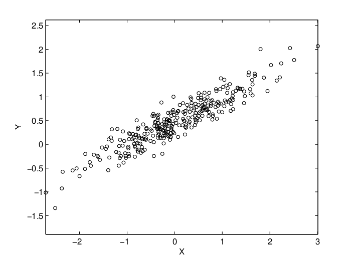
For each notion of the aforementioned regression depths, we plot two figures, namely, a 3-dimensional depth plot and its corresponding contours over $\bm{\theta}=(\beta_{0},\beta_{1})^{\top}\in[0,1]\times[0,1]$; see Figures 2 - 6. Seven contours, as well a maximizer of each regression depth function (see the big point in the center), are reported. The figures shows that, except the sample Rayleigh regression depth, all reported depth contours of these four depth functions are not convex, but still roughly nested, and their shape is data-dependent. Generally speaking, among these four depths, the contours of projection regression depth appears to be smoother than those of the halfspace and simplicial regression depth, but rougher than those of the zonoid regression depth. Furthermore, the roughly nested construction of contours indicates that the value of all regression depths tends to become smaller when $\bm{\theta}$ is moving from the center to outside, although it may be not strictly decreasing for, e.g., halfspace regression depth. One exception is the Rayleigh regression depth. Its sample contours are some nested ellipses, which coincides with the Theorem 4.

Furthermore, all maximizers of these five regression depth functions are very closed to the true coefficient parameter $\bm{\theta}_{0}=(0.5,0.5)^{\top}$ in this example. It indicates that, relying on any of them, we are able to develop a proper median-like estimator for the unknown regression efficient.

In this paper, we investigated the possibility of generalizing some usual depths into the regression setting. A general concept of regression depth was proposed. Several new regression depth notions, such as projection regression depth, were suggested relying on a further look at the relationship between the halfspace regression depth of Rousseeuw and Hubert (1999) and Tukey’s location depth.

Unfortunately, it turns out that the halfspace, simplicial, projection, zonoid regression do not satisfy Q3 of 2. Hence, using these four depth notions, it is probably impossible to induce a strictly decreasing ordering when the parameter $\bm{\theta}$ is moving along any line stemming from the center $\bm{\theta}_{0}$ to outside.

However, the results of Theorems 1-5, as well as the illustrations given in Section 5, indicate that it is still possible to induce some median-like estimators relying on these depth nations. In the literature, it is well known that the breakdown point robustness of the projection median is much higher than that of Tukey’s halfspace median (Zuo, 2003). Hence, we anticipate that this is also the case for projection regression depth, and will pursuit it in the future. On the other hand, the Rayleigh regression depth satisfies Property Q3, confirmed by Figure 5. In this sense, if the main purpose is to provide a full ordering like in the location setting, one may use the Rayleigh regression depth.

Observe that the computational issue is usually concerned by practitioners related to statistical depth functions. Fortunately, the depth value of all regression depth notions mentioned in this paper is computable, because their definitions are based on their counterparts in the location setting, thanking to the latest developments of the computation of halfspace depth (Liu and Zuo, 2014a; Dyckerhoff and Mozharovskyi, 2016), projection depth (Liu and Zuo, 2014b), and zonoid depth (Mosler et al., 2009), and so on. We refer reads to Pokotylo et al. (2016) for details of a R package ddalpha, which includes implementations of most depth notions in the location setting.

The research is supported by NNSF of China (Grant No.11601197, 11461029), China Postdoctoral Science Foundation funded project (2016M600511, 2017T100475), NSF of Jiangxi Province (No.20171ACB21030, 20161BAB201024), and the Key Science Fund Project of Jiangxi provincial education department (No.GJJ150439).

In this appendix, we provided the detailed proofs of the main proposition and theorems.

References

- Bai and He (1999) Bai, Z.D., He, X.M., (1999). Asymptotic distributions of the maximal depth estimators for regression and multivariate location. Ann. Statist., 27: 1617-1637.
- Cascos and Molchanov (2007) Cascos, I., Molchanov, I. (2007). Multivariate risks and depth-trimmed regions. Finance and stochastics, 11(3), 373.
- Chenouri et al. (2011) Chenouri, S., Small, C., Farrar, T. (2011). Data depth-based nonparametric scale tests. Canadian Journal of Statistics, 39(2), 356-369.
- Christmann et al. (2002) Christmann, A., Fischer, P., Joachims, T. (2002). Comparison between various regression depth methods and the support vector machine to approximate the minimum number of misclassifications. Comput Stat 17:273-287.
- Dyckerhoff and Mozharovskyi (2016) Dyckerhoff, R., Mozharovskyi, P., (2016). Exact computation of the halfspace depth. Comput. Statist. Data Anal., 98, 19-30.
- Einmahl et al. (2015) Einmahl, J. H., Li, J., Liu, R. Y. (2015). Bridging centrality and extremity: Refining empirical data depth using extreme value statistics. The Annals of Statistics, 43(6), 2738-2765.
- Ghosh and Chaudhuri (2005) Ghosh, A. K., Chaudhuri, P. (2005). On maximum depth and related classifiers. Scandinavian Journal of Statistics, 32(2), 327-350.
- He and Einmahl (2017) He, Y., Einmahl, J. H. (2017). Estimation of extreme depth-based quantile regions. Journal of the Royal Statistical Society: Series B (Statistical Methodology), 79(2), 449-461.
- Hu et al. (2011) Hu, Y., Wang, Y., Wu, Y. (2011). Tensor-based projection depth. Bernoulli, 17(4), 1386-1399.
- Hubert et al. (2016) Hubert, M., Rousseeuw, P., Segaert, P. (2016). Multivariate and functional classification using depth and distance. Advances in Data Analysis and Classification, 1-22.
- Lange et al. (2014) Lange, T., Mosler, K., Mozharovskyi, P. (2014). Fast nonparametric classification based on data depth. Statistical Papers, 55(1), 49-69.
- Li et al. (2012) Li, J., Cuesta-Albertos, J.A. and Liu, R.Y. (2012). -classifier: nonparametric classification procedure based on -plot. Journal of the American Statistical Association, 107, 737-753.
- Liu (1990) Liu, R. Y. (1990). On a notion of data depth based on random simplices. Ann. Statist., 18: 191-219.
- Liu et al. (1999) Liu, R. Y., Parelius, J. M., Singh, K. (1999). Multivariate analysis by data depth: descriptive statistics, graphics and inference, (with discussion and a rejoinder by Liu and Singh). The annals of statistics, 27(3), 783-858.
- Liu and Zuo (2014a) Liu, X., Zuo, Y. (2014a). Computing halfspace depth and regression depth. Communications in Statistics-Simulation and Computation, 43, 969-985.
- Liu and Zuo (2014b) Liu, X., Zuo, Y. (2014b). Computing projection depth and its associated estimators. Statistics and Computing, 24(1), 51-63.
- Liu et al. (2017) Liu, X., Zuo, Y., Wang, Q. (2017). Finite sample breakdown point of Tukey’s halfspace median. Science China Mathematics, 60(5), 861-874.
- Kong and Zuo (2010) Kong, L., Zuo, Y. (2010). Smooth depth contours characterize the underlying distribution. Journal of Multivariate Analysis, 101(9), 2222-2226.
- Koshevoy and Mosler (1997) Koshevoy, G., Mosler, K. (1997). Zonoid trimming for multivariate distributions. The Annals of Statistics, 1998-2017.
- Massé (2009) Massé, J.C. (2009). Multivariate Trimmed means based on the Tukey depth. Journal of Statistical Planning and Inference, 139(2), 366-384.
- Mosler (2013) Mosler, K. (2013). Depth statistics. In Robustness and complex data structures (pp. 17-34). Springer Berlin Heidelberg.
- Mosler et al. (2009) Mosler, K., Lange, T., Bazovkin, P. (2009). Computing zonoid trimmed regions of dimension . Comput. Statist. Data Anal. 53, 2500-2510.
- Paindaveine and Van Bever (2015) Paindaveine, D., Van Bever, G. (2015). Nonparametrically consistent depth-based classifiers. Bernoulli, 21(1), 62-82.
- Pokotylo et al. (2016) Pokotylo, O., Mozharovskyi, P., Dyckerhoff, R. (2016). Depth and depth-based classification with R-package ddalpha. arXiv preprint arXiv:1608.04109.
- Rousseeuw and Leroy (1987) Rousseeuw, P.J. Leroy, A. (1987). Robust regression and outlier detection. Wiley New York, 1987.
- Rousseeuw and Hubert (1999) Rousseeuw, P.J., Hubert, M. (1999). Regression depth (with discussion). J. Amer. Statist. Assoc., 94: 388-433.
- Rousseeuw and Hubert (2015) Rousseeuw, P. J., Hubert, M. (2015). Statistical depth meets computational geometry: a short survey. arXiv preprint arXiv:1508.03828.
- Tukey (1975) Tukey, J.W. (1975). Mathematics and the picturing of data. In Proceedings of the International Congress of Mathematicians, 523-531. Cana. Math. Congress, Montreal.
- Van Aelst et al. (2002) Van Aelst, S., Rousseeuw, P. J., Hubert, M., Struyf, A. (2002). The deepest regression method. Journal of Multivariate Analysis, 81(1), 138-166.
- Wei and Lee (2012) Wei, B., Lee, S. M. (2012). Second-order accuracy of depth-based bootstrap confidence regions. Journal of Multivariate Analysis, 105(1), 112-123.
- Wilcox (2010) Wilcox, R. R. (2010). Comparing non-parametric regression lines via regression depth. Journal of Statistical Computation and Simulation, 80(4), 379-387.
- Yeh and Singh (1997) Yeh, A., Singh, K. (1997). Balanced confidence regions based on Tukey’s depth and the bootstrap. Journal of the Royal Statistical Society: Series B (Statistical Methodology), 59: 639-652.
- Zuo and Cui (2005) Zuo, Y., Cui, H. (2005). Depth weighted scatter estimators. Annals of Statistics, 381-413.
- Zuo and Serfling (2000a) Zuo, Y., Serfling, R. (2000a). Nonparametric notions of multivariate “scatter measure” and “more scattered” based on statistical depth functions. Journal of Multivariate analysis, 75(1), 62-78.
- Zuo and Serfling (2000b) Zuo, Y., Serfling, R. (2000b). General notions of statistical depth function. Ann. Statist., 28: 461-482.
- Zuo and Serfling (2000c) Zuo, Y., Serfling, R. (2000c). On the performance of some robust nonparametric location measures relative to a general notion of multivariate symmetry. Journal of Statistical Planning and Inference, 84(1), 55-79.
- Zuo (2003) Zuo, Y. (2003). Projection based depth functions and associated medians. Ann. Statist., 31: 1460-1490.
- Zuo et al. (2004) Zuo, Y., Cui, H., He, X.M. (2004). On the Stahel-Donoho estimators and depth-weighted means for multivariate data. Ann. Statist. 32(1), 189-218.