MULTI-WAVELENGTH STELLAR POLARIMETRY OF THE FILAMENTARY CLOUD IC5146: I. DUST PROPERTIESFacilities: ARIES:ST, LO:1m, Perkins
Abstract
We present optical and near-infrared stellar polarization observations toward the dark filamentary clouds associated with IC5146. The data allow us to investigate the dust properties (this paper) and the magnetic field structure (Paper II). A total of 2022 background stars were detected in -, -, -, and/or -bands to mag. The ratio of the polarization percentage at different wavelengths provides an estimate of , the wavelength of peak polarization, which is an indicator of the small-size cutoff of the grain size distribution. The grain size distribution seems to significantly change at 3 mag, where both the average and dispersion of decrease. In addition, we found 0.6–0.9 m for mag, which is larger than the 0.55 m in the general ISM, suggesting that grain growth has already started in low regions. Our data also reveal that polarization efficiency (PE ) decreases with as a power-law in -, -, and -bands with indices of -0.710.10, -1.230.10 and -0.530.09. However, -band data show a power index change; the PE varies with steeply (index of -0.950.30) when mag but softly (index of -0.250.06) for greater values. The soft decay of PE in high regions is consistent with the Radiative Aligned Torque model, suggesting that our data trace the magnetic field to mag. Furthermore, the breakpoint found in -band is similar to the where we found the dispersion significantly decreased. Therefore, the flat PE- in high regions implies that the power index changes result from additional grain growth.
Keywords:
dust, extinction — ISM: clouds — ISM: magnetic fields — ISM: structure — ISM: individual objects (IC5146) — PolarizationI INTRODUCTION
The linearly polarized background starlight observed in early studies [29, 33], was suggested to result from dichroic absorption by non-spherical dust grains aligned to B-fields [34]. Hence, polarized starlight is commonly used as a tracer of the B-field structure in the plane of sky [9, 15, 25, e.g.,]. The first theory to explain dust alignment utilized a paramagnetic mechanism (DG alignment) [20]. However, later studies revealed time-scale and efficiency problems, so other alignment mechanisms were offered, including superparamagnetic grains [39] and superthermal rotation rates [61]. But most of these are efficient only for particular physical conditions and fail to explain the polarization observed across the wide variety of environments (see review in Andersson et al. 4).
Radiative Aligned Torques (RATs) [21, 22, 23, 48] is currently the best model to explain how dust grains align with B-fields. The RATs theory assumes an anisotropic radiation field impacting non-spherical dust grains. The radiation field can generate net torque on the grains and induce both spin of the grains and precession about the B-field. For typical interstellar radiation fields, the RATs alignment timescale is much faster than DG alignment [48], and superthermal rotation tends to enhance RATs alignment more than DG alignment [36]. In addition, RATs is efficient across a variety of environments, and thus more likely dominating the grain alignment process.
A key prediction of RATs theory is the decreasing polarization efficiency (PE, Pλ/) with increasing , because the radiation field required to align the dust grains is decreased due to extinction [47]. In order to examine whether the RATs theory can explain observed polarizations, Whittet et al. [82] performed a numerical simulation, based on RATs theory, and assuming a starless core with only an external radiation field and a fixed dust grain size distribution for all . Their simulation results matched their -band polarimetry data toward Taurus up to at least mag; the -band polarization degree varied with as a power-law, with . In addition, their simulation predicted the RATs mechanism would cease as approached 10 mag, since the radiation that can penetrate to such high column densities has wavelengths too long to effectively align the grains. However, the single power-law well matched their data over the 0–30 mag range, which was inconsistent with the predicted cessation of alignment at 10 mag. To explain the inconsistency, Whittet et al. [82] argued that the RAT mechanism may still work in high regions if: (1) the dust grains have undergone significant growth, and so can couple to longer wavelength radiation, or; (2) embedded stars are present to provide radiation at shorter wavelength to enhance the alignment of small dust grains.
To further test the RATs theory in dense clouds, Jones et al. [42] used both infrared and submillimeter polarimetry data to trace the variation of polarization efficiency up to mag within starless cores. They found a change of power-law index for polarization efficiency versus extinction from -0.5 to -1 at mag, consistent with the cessation of alignment predicted by Whittet et al. [82]. In addition, Jones et al. [43] found a deeper break point at hundreds mag and a reversed trend such that the power-law index of polarization efficiency versus changed from -1 to -0.5 within the Class 0 YSO G034.43+00.24 MM1. The opposite trends shown in these two cases suggest that dust alignment in dense clouds could be strongly affected by environmental effects.
In the RATs paradigm, the polarization degree is expected to be wavelength-dependent, because the cloud extinction penetration is wavelength-dependent and because the highest alignment efficiency occurs at wavelengths similar to the sizes of the grains [11, 48]. Therefore, the polarization wavelength-dependence is determined by both the extinction and the size of dust grains, resulting in a polarization spectrum exhibiting a single peak (). Kim & Martin [44] showed that is sensitive to the small-size cutoff of the grain size distribution, since the dust size distribution is a power-law and the small-size cutoff will effectively determine the mean size of the dust grains. Whittet et al. [82] calculated the variation with using a RATs model with a fixed grain size distribution over , and showed that the RATs theory can explain their observed dependence of increasing with to 6 mag, but that RATs predicts should flatten for larger in the Taurus cloud.
Recent observational results are mostly consistent with RATs theory (Whittet et al. 82, Alves et al. 2, Cashman & Clemens 8), although the dust alignment efficiency varies from source to source. As an extreme case, Goodman et al. [27] found a constant near-infrared polarization degree toward L1755 for of 1–10 mag, and argued that near-infrared polarization can only trace the B-field on the surfaces of dark clouds. In contrast, other observations mostly showed polarization degree increasing with , such as toward Taurus [82] and toward L204 cloud 3 [8], suggesting that the constant polarization degree found in Goodman et al. [27] represented a special case and was not the norm.
It is still unclear why the P- relation found in L1755 is different from the relation found for other clouds. Whittet et al. [82] re-analyzed the L1755 polarimetry data with better background star selection and extinction estimation, but still found the same relation. They speculated that this unique relation might result from a lack of the typical physical conditions leading to grain alignment inside this cloud or a reduction of observed polarization due to complex B-field structure within the L1755 filaments. To examine these possibilities, more polarimetry observations covering both a wider area and more wavebands could help to reveal the alignment conditions for dust grains with different sizes and to probe the detailed B-field structure. In addition, since the Goodman et al. [27] polarization detections only spanned a small range of (2–8 mag), it would be of interest to perform polarization observations with higher sensitivity to investigate this relation to higher values.
An ideal target for detailed testing the RATs paradigm is the system of dark cloud filaments associated with the reflection and emission nebula IC5146, a nearby ( 460 pc) star-forming region in Cygnus. The system consists of a young cluster inside an HII region and a long, main, dark cloud filament with several sub-filaments branching out from the main filament. The Herschel Gould Belt Survey [5] revealed a complex network of filaments within the long dark cloud highlighting the locations of young forming stars. The Planck polarization map of IC5146 [60] revealed that the B-field is nearly uniform, with the mm-wavelength-traced B-field oriented perpendicular to the elongation orientation of the main filament. Such an apparently uniform B-field gives the IC5146 dark cloud system an advantage for testing the RATs model, because the high angular resolution of stellar polarizations can be used to test for, and quantify, complex B-fields along the multiple line of sights.
In a series of papers, we will report measurements and analyses of the polarizations of stars behind the IC5146 filamentary cloud. The polarimetry of background starlight was performed at both optical and infrared wavelengths to probe the large-scale B-field in the cloud. In this paper, we focus on the dust properties and the dust alignment conditions revealed by our data in order to identify where the B-fields were accurately probed by our observations. The observations and data reduction are described in Section II. In Section III, we present the polarization measurements toward IC5146. Section IV presents an initial analysis of the data to show how the dust grain alignment conditions vary with and regions. In Section V, we discuss the evolution of dust grains and how the dust properties influence the polarization efficiency. The consequences of these results to the investigations of the role of B-fields in cloud evolution will be offered in the forthcoming Paper II.
II OBSERVATIONS AND DATA REDUCTION
We measured the polarization of background stars toward the IC5146 filamentary cloud system with several instruments; Aryabhatta Research Institute of Observational Sciences (ARIES) Imaging Polarimeter (AIMPOL; Rautela et al. 62) and Triple-Range (, , ) Imager and POLarimeter (TRIPOL; Sato et al. 65, Sato et al. 66) provided optical - and -band polarimetry data, respectively. Mimir [13] measured the - and -band polarizations at near-infrared wavelengths. Figure 1 shows the target fields for each instrument overlaid on the Herschel archive 250 m image [28, 5]. The dust continuum map shows an east-west main filament connected to the bright cluster complex, known as the Cocoon Nebula. Numerous “sub-filaments” are extended from the main filament, with the largest sub-filament located on the north-west side of the main filament. Almost all parts of the cloud were observed with Mimir, while the fields observed with AIMPOL were chosen to be mainly in the edge of the cloud in order to cover as many optically bright stars as possible. The TRIPOL observations focused on the northwestern region, with longer exposure time, where bright stars are rare both at optical and infrared wavelengths. The detailed information of the observations with the different instruments are described below.
II.1 AIMPOL Polarimetry
The -band (0.67m, bandwidth=0.14 m) polarimetric observations were carried out toward the IC5146 filamentary cloud system using AIMPOL mounted at the Cassegrain focus of the 104-cm Sampurnanand telescope of the ARIES, Nainital, India. AIMPOL consisted of a half-wave plate (HWP) modulator and a Wollaston prism beam-splitter illuminating a fraction (370370 pixel2) of the Tektronics 10241024 pixel2 CCD camera. The pixel size of the CCD was 1.73″ and the typical seeing was 2″. The observations spanned the nights of 2011 November 4–8 and 2012 November 8–15 and covered 37 fields (see Figure 1) with each field having a useful diameter of 8′. In order to obtain Stokes Q and U, we took images at four independent HWP orientations (, , , and ; Schaefer et al. 69). The Wollaston prism analyzer produced offset, but simultaneous, ordinary and extraordinary overlapping images for each HWP orientation. Hence, each image resulted in one measurement of Stokes Q or U. The integration time was set to 10 minutes for each HWP orientation, so the total integration time for each field was 40 minutes.
The polarization measurements were calibrated for instrumental polarization and offset angle by observing standard polarized and unpolarized stars drawn from Schmidt et al. [70]. The data were reduced using standard IRAF procedures 11 1 IRAF is distributed by the National Optical Astronomy Observatory, which is operated by the Association of Universities for Research in Astronomy (AURA) under a cooperative agreement with the National Science Foundation.. The fluxes in the ordinary and extraordinary beams for each observed source were extracted using standard aperture photometry. Sources with stellar overlap, less than 10% of the total sources, were excluded. The polarization degree and angle for each star were derived from the relative fluxes in the ordinary and extraordinary beams. We removed the Ricean bias with the asymptotic estimator
| (1) |
where is the debiased degree of polarization, and are normalized Stokes and , and is the uncertainty in the polarization percentage [78]. The details of the observing facility and procedures used to estimate the polarization degree and polarization angles (P.A.) are described in Eswaraiah et al. [24], Eswaraiah et al. [25].
II.2 TRIPOL Polarimetry
Polarimetric observations focused on the northwestern region of IC5146 in -bands (0.77 m, bandwidth 0.15 m) on 2012 July 27–28 and 2014 July 6 with TRIPOL installed on the Lulin-One-meter Telescope in Lulin Observatory, Taiwan. Seven fields, each with size of 4′4′, were observed (see Figure 1). TRIPOL consisted of dichroic mirrors and three ST-9 512512 pixel2 CCD cameras, which enabled simultaneous observations in -, -, and - bands; however, only the -band data were able to detect background stars behind this dark cloud. The pixel sizes of the CCDs were 0.5 arcsec and the average seeing was 1.5″. A rotatable achromatic half wave-plate and a fixed wire-grid were used to analyze the incoming light. Each field was measured at four HWP orientations (, , , and , with pairs of images yielding stellar Stokes Q and U values.). The integration time for each position angle was 22.5 minutes, so each field required a total of 1.5 hours.
Standard reduction procedures were applied using IRAF, and the photometry of each background star was obtained using Source Extractor [7]. The debiased polarization degree and angle for each background star were derived from the fluxes measured through each of the four HWP orientation angles and calibrated against observations of polarized and unpolarized standard stars from Schmidt et al. [70].
II.3 Mimir Polarimetry
We carried out - (1.6 m) and -band (2.2 m) polarization observations toward IC5146 on 2013 September 17–27, using the Mimir instrument [13] mounted on the 1.8 m Perkins telescope located near Flagstaff, AZ and operated by Lowell Observatory. Fifty-seven fields covering IC5146 cloud were observed in -band, and twelve fields were observed in -bands toward the dense regions (see Figure 1). The pixel size of the InSb detector array was 0.58 arcsec and the average seeing was 1.5″. The field of view was 10′10′ for Mimir, and we set 1′ overlap between adjacent fields. Each field was observed in six sky dither positions where images were taken at 16 orientation angles of the HWP. A total of 96 (166) images were taken for each field with 10 sec of integration time for each image for both - and -bands, and thus the total integration time was 16 minutes for each field. We took an additional short integration for those fields with bright stars, which took 4 minutes per field.
In order to calibrate the non-linearities of the InSb detector array, a series of images were taken with an increasing exposure time toward an illuminated flat-field screen, and the response curve of each pixel was fitted with a polynomial model to obtain a linearity correction. Flat fields for each HWP position were taken using a lights-on/lights-off method toward a flat field screen inside the closed dome during the observation run. The data were calibrated using the Mimir Software Package Basic Data Processing (MSP-BDP), and the Photo POLarimetry tool (MSP-PPOL) was used to extract Stokes Q and U values for each observed source from the calibrated data. The detailed processes used in the Mimir Software Package are described in Clemens et al. [15], Clemens et al. [16], Clemens et al. [17].
III RESULTS
III.1 The Polarization Catalog
We matched the polarization data to the 2MASS catalog [71] to obtain positions accurate to 0.5 arcsec. Table 1 lists all the observed polarization properties as well as photometric magnitudes from 2MASS and WISE [84]. Column 1 lists the star number, and column 2 and 3 list the RA and Dec. The measured Stokes Q, U, debiased P, and position angle P.A. in -, -, -, and -bands with their uncertainties are listed in columns 4–35. The J-, -, -, W1-, and W2-band magnitudes and uncertainties are listed in columns 36–45. Column 46 presents the estimated visual extinction described in Section IV.1. Column 47 present the Usage Flag (UF; stars with UF=1 were selected for further analyses, and stars with UF=0 were not used). The usage data were selected with polarization degree divided by its uncertainty for - and -bands, and and 5 % for - and -bands; the selection criteria were relaxed for near-infrared data, since the number of 3 near-infrared detections were too few for adequate statistics.
In total, 2022 independent background stars have polarization detections in at least one of the four bands, 239 stars were detected in 2 bands, 24 stars were detected in 3 bands, and only 3 stars were detected in all four bands. About 71 of the background stars were detected in -band, 24 in -band, 10 in -band, and 8 in -band.
Figure 2shows all of the polarization measurements on the Herschel SPIRE 250 m image. The inferred B-field is seemingly perpendicular to the main filament on large scales but parallel to the sub-filaments. The bimodal perpendicular or parallel alignment is similar to that seen in previous polarimetry work toward filamentary clouds, and has been ascribed to B-field confinement of sub-Alfvénic turbulence or gravitational contraction channeled by strong B-fields [50]. We will discuss the B-field structure in detail and estimate the B-field strengths with the Chandrasehkar-Fermi method to determine the dynamical importance of the B-fields in Paper II.
III.2 Consistency in P.A. between Multiple Wavelengths
To test whether the results from AIMPOL, TRIPOL and Mimir were consistent, and thereby capable of revealing wavelength-dependent effects in the probed dust columns, we selected the stars with detections at multiple wavelengths, and examined their P.A.s in the different wavelength in Figure 3. In total, 143, 31, and 65 stars were selected in -, -, and - band pairs. The mean P.A. differences in these three band pairs were -4.60.8°, 6.20.8°, and -2.91.6°, respectively. The standard deviation of the measured P.A. differences were 8.7°, 16.3°, and 26.6° for -, -, and - band pairwise samples. The average expected uncertainties of P.A. difference, propagated from observational uncertainties (), were 4.2°, 9.3°, and 12.3° for -, -, and - band pairwise samples. The P.A. difference standard deviations obtained from these sets are 1–2 times to the propagated instrumental uncertainties, which are acceptable values since the P.A.s may be intrinsically different at different wavelength because they may trace the polarizations to different depths.
III.3 Negligible Foreground Contamination
We attempted to identify and exclude foreground stars whose polarizations are not tracing the B-field of the IC5146 cloud system. To obtain enough star samples to represent the foreground polarization near IC5146, we selected stars having known distances, and -band polarization measurements from van Leeuwen [75] and Heiles [31], within a 10° radius sky area near IC5146. Figure 4 shows the -band polarization degree (PV) vs. distance for these 41 stars. The distance of pc to the IC5146 cloud system [46] was used to separate these stars into foreground and background groups. The polarization degree rises significantly at a distance of pc, possibly due to nearby clouds in the Gould Belt. For most of the stars with distances less than 400 pc, the polarization degrees are below 0.3. This value was chosen as the upper limit of the foreground -band polarization for the sky area near IC5146.
In the ISM, the polarization in the -band is greater than in the Rc-, - or -bands [67]. Hence, based on the foreground star values in Figure 4, the foreground polarization in the Rc-, -, and -bands are expected to be less than %. This foreground polarization upper limit is similar to the instrumental uncertainties of our data (). Hence, any foreground stars were likely to have been already excluded by our selection criteria ( 3 for - and -bands and 2 for - and -bands). Thus, we concluded that contamination by foreground stars was negligible in our sample set, and further that no foreground polarization correction to the remaining data was necessary.
IV ANALYSIS
IV.1 NICER Extinction
Visual extinction provides an estimate of how many dust grains are responsible for the observed starlight polarization, and thus is required for estimating dust alignment efficiency and testing RATs theory. We used the Near-Infrared Color Excess Revisited (NICER) technique [51]22 2 Using the PNICER python package developed by Meingast et al. [56] to calculate the visual extinction over the IC5146 cloud system. The NICER technique utilizes multi-band colors to obtain extinction for a target field, using extinction coefficients derived from Indebetouw et al. [37]. We selected a total of 186,319 stars from the 2MASS catalog and 46,100 stars from the WISE catalog covering the IC5146 cloud system. To estimate the stellar intrinsic colors, a square control field, centered at RA=330.153°, Dec=+47.794° with a side length of 15′, was compared to the target field.
To examine the quality of the extinctions estimated, the NICER extinction map shown in Figure 5 was created and compared with the Herschel map. The extinction map was created from the variance-weighted mean of NICER extinction of each individual star within a pixel grid having a pixel size of 30″. The pixel grid was smoothed using a Gaussian weighting kernel with FWHM of 90″. The black contours in Figure 5 show the Herschel 250 m data. The morphology of the extinction map is almost identical to that of the 250 m map.
Figure 6shows the histogram of values derived from the NICER analysis. The uncertainties in arise both from the uncertainties of the spectral types and from the propagated photometric uncertainties. In order to estimate the overall uncertainty of , we selected all the stars that NICER assigned with negative , and assumed that the negative values were only due to uncertainties. This negative portion of the full distribution was duplicated and reflected about =0 to generate a new pseudo distribution. Fitting this with a Gaussian centered at =0, we derived a standard deviation of 0.93 mag. Because this includes uncertainties from both spectral typing and observations, we adopted this value as our uncertainty.
IV.2 Polarization Efficiency
To test whether the polarization measurements trace the magnetic field structure inside the IC5146 cloud system, we examined whether embedded dust grains align with the B-fields via estimating how the degree of polarization varied with extinction. Polarization efficiency (PE) is defined as polarization percentage divided by . It describes how much polarization is contributed by dust grains in the line of sight. We used PE versus to test whether the dust grains are better aligned in the diffuse region, as predicted by the RATs model.
Figure 7shows PE versus for the -band data. The data probability density over the PE- space, represented by the contours, was calculated using Kernel Density Estimation [64, 59]; for each source, the probability distribution function was described by a Gaussian kernel, and the width of the Gaussian kernel was determined by the uncertainties of PE and . The probability density for the entire data set was represented by the summation of the Gaussian kernels.
To reduce the uncertainty from and also avoid the bias due to uneven sampling over , the variance-weighted means of PE and were calculated in bins of width log() = 0.1. The uncertainties of the weighted mean of PE and for each bin were propagated from the instrumental uncertainty and uncertainty for each sample. Those stars that NICER assigned with negative were not used for PE determination, since their extinctions were negligible.
Similarly, PE versus plots for the -, -, and -bands are shown in Figure 8, Figure 9, and Figure 10, respectively. In -band, the last bin ( = 5 mag) was found to have significantly higher PE and the bin only contained two stars. This bin was judged to be an outlier, and was excluded from further analysis. In the four bands, PE always decreased with but with different slopes. In addition, the PE at mag is still half of the PE at mag, suggesting that the dust grains in high regions are still being aligned with some degree of efficiency.
The power-law behavior of PE- has been shown in previous studies [82, 9, 8, e.g.,], and apears to be well matched to the prediction of RATs theory. However, recent studies have also discovered changes in the index of the power-law for high extinction regions [2, 4]. To test whether, in the IC5146 dark cloud system, the power-law index changes with , we fit Pλ/ versus with both a single power-law (hereafter, Model 1):
| (2) |
and with a broken power-law (hereafter, Model 2):
| (3) |
where =. The four parameters, , , and , and , were all taken as free parameters in the fit to the Model 2.
The goodness of fit on the binned data to the two models was examined using the F-test and the bias-corrected Akaike information criterion (AICc, Akaike 1, Sugiura 73). The two different model comparison methods may exhibit different preferences. For example, Ludden et al. [52] used Monte Carlo simulations to examine the performance of these methods, finding that the F-test tends to choose the simpler model more often than does the AICc even when the more complex model is correct. To avoid possible bias, we used both methods to compare the model fits, and the preferred Model was chosen to be the one which (1) the F-test probability is below 0.05 (95% confidence level) and (2) has lower AICc value. The results of the fitting and model comparisons are listed in Table 2. Both the F-test and AICc show consistent results; the broken power-law is the better model for -bands, and the single power-law is the better model for -, -, and -bands.
The PE- relations were empirically found to be insensitive to observing wavelengths [e.g., 4, and references therein], although our observed PE- relations might be expected to show some differences among the observing bands, since each data set covered different and spatial ranges. The - and -band data mostly probed the regions with 4 mag, and thus the derived PE indices mainly characterize the low regions. The power index of for -band is very different from the index for the -band, namely . In addition, the power index of for -band for low values is in between the indices for -band and -band. For high regions, the index of for -band is softer than the index for -band (), and both are flatter than all of the indices characterizing low regions. This finding may indicate that the physical properties of grains, as well as their alignment efficiencies, change significantly beyond –4 mag (see Section V.4)
The -, -, and -band data all covered the mag regime; however, the power-law indices for these three bands were all different. One major difference between the -, -, and -band data was that the -band observations covered almost all of the IC5146 cloud system while the -band observations mostly covered the main filament, and the -band observations only probed the north-west filament (see Figure 1).
To test whether the indices characterizing low regions differ from region to region, the stars with -band detections and mag were assigned to one of the five zones delineated in Figure 11. Within each zone, single power-law indices were derived and are shown in Figure 11. Power-law indices ranging from to were fit to the assigned -band data within the different zones. The indices were significantly softer in the eastern part of the cloud than in the western and northern part. In addition, the index derived within the northern zone was -1.180.14, nearly identical to the index for -band, namely , covering a substantially similar region. Hence, the PE- relation varies by region in the low extinction regions. The different indices derived for the different wavelengths for the whole cloud could then merely arise from the combination of a variety of PE- relations. The possible origin of the diverse PE relation is discussed further in Section V.3.
IV.3 Wavelength Dependence of Polarization using the Serkowski relation
The polarization of starlight is known to be wavelength-dependent, resulting in a polarization spectrum. Since this wavelength-dependence originates from dust properties and alignment conditions, the polarization spectrum can be used to investigate the evolution of dust grains. The polarization spectrum is well-fit by the empirical “Serkowski relation,”
| (4) |
where is the peak polarization degree at wavelength [67]. In later studies, the parameter K was shown to follow the relation c [83], where c was found to depend on dust properties, such as geometric shape [76, 77, e.g.,].
To fit the Serkowski relation for its three parameters, detections in at least four bands are required to obtain uncertainties in the parameters. However, it is difficult to do so in the presence of high extinction. Thus, most of the previous studies have been limited to low extinction regions. Even among our data, only three stars were detected in all four wavebands. The Serkowski relation fit results for these stars are shown in Figure 12. The range of fitted is 0.72–0.83 m, significantly greater than the typical value m characterizing the general diffuse interstellar medium [68].
IV.4 “Polarization color” as a constraint on
It is difficult to obtain the necessary multiple wavelength polarization detections needed to fit Serkowski relations in the presence of strong extinction. In order to have more samples to constrain , we examined the “polarization color” (ratio of polarization degrees at two bands) as a partial descriptor of the polarization spectrum. Polarization color can be easily obtained from a limited set of wavebands without presumption of the spectrum shape. The Serkowski relation has been suggested to be only valid for a limited wavelength range, mostly UV through optical. Martin [53] found the polarization spectrum between 1.6–5 m wavelength behaved more like a power-law than like the Serkowski relation, and Clayton et al. [12] found the polarization spectrum in the ultraviolet showed an excess with respect to the Serkowski relation.
In the wavelengths where the Serkowski relation is valid, polarization color can constrain . Following the Serkowski relation, the ratio of polarization degree of a star at two wavelengths can be written as:
| (5) |
To reduce the free parameters, we also assumed the relation K= c, where c is expected to be a constant over . Via Equation 5 and the assumptions regarding K, polarization color (ratio) is determined by only one free parameter, . Thus, only one polarization color is required to constrain , although for wavebands right near , the uncertainties will be large. Clemens et al. [18] used this approach with Mimir - and -band data to identify grain growth in the moderate to high extinction regions of L1544, finding in the 1.0-1.2 m range.
The polarization color versus values shown in Figure 13 reveal how the polarization spectrum varies with . The observed distribution seems diverse and could be hardly described with a simple function. To try to find some order, we separated the stars into four groups by eye, based on the similarities in the distribution. They span ranges of , 1.0–2.5, 2.5–4.0, and 4.0 mag, labelled as regions “A”, “B”, “C”, and “D”, respectively. The blue horizontal lines show the unweighted averagestandard deviation (STD) of for each group. The intrinsic dispersions of were derived using , where was the average observational uncertainty. The statistical properties of for each group are presented in Table 3.
Group A had significantly lower mean than the other regions. Since the of this region was comparable to expected foreground extinction 0.3 mag [45], the depolarization due to any foreground medium might significantly affect the polarization spectrum. Thus, the polarization color in this group might not accurately trace the dust properties. The average values for group B, C, and D were similar to each other, although significant intrinsic dispersion was found for group B.
The value of directly determines the value of if the parameter c in Equation 5 is known. The variance-weighted mean c of 2.3 was derived from the four-band fitting to the three stars shown in Figure 12. This c value was higher than the value of 1.66 found in Wilking et al. [83] and the value of 1.86 found in Whittet et al. [80]. Figure 14 shows how maps to for different value of c. The black horizontal dashed lines delimit the span of the distribution of values found in Figure 13. The curves in Figure 14 characterized by c 2.1 cannot cover the full range of the distribution of observed values, suggesting that the parameter c value in IC5146 cloud system is likely higher than it is in other clouds. Hence, we assumed c 2.3 to estimate the from observed .
The range of versus , for c 2.3, is shown in Figure 15. The mean for the mean in each of the four groups is listed in Table 3. For each , two possible solutions from the Serkowski relation are possible, as can been seen in Figure 14. These two solution regions were colored in gray regions for the lesser values and in red for the greater values. If we assume that across the cloud system does not dramatically change within a few magnitudes of extinction, then only one set of solutions is likely to be true. Since the values of derived from the four-band fitting to the three stars shown in Figure 12 were all in the range of 0.72–0.83 m, 0.4 m selects the better solutions.
Hence, the average values correspond to of 0.75, 0.78, and 0.73 m for groups B, C, and D, respectively. These are all greater than the average value for the ISM of 0.55 m [68], suggesting that the dust grains across most of the IC5146 cloud system have grown significantly with respect to dust grains in the diffuse ISM. In addition, the large dispersion of in group B implies that the dust grain size distributions are more diverse in this range than in the other extinction regions.
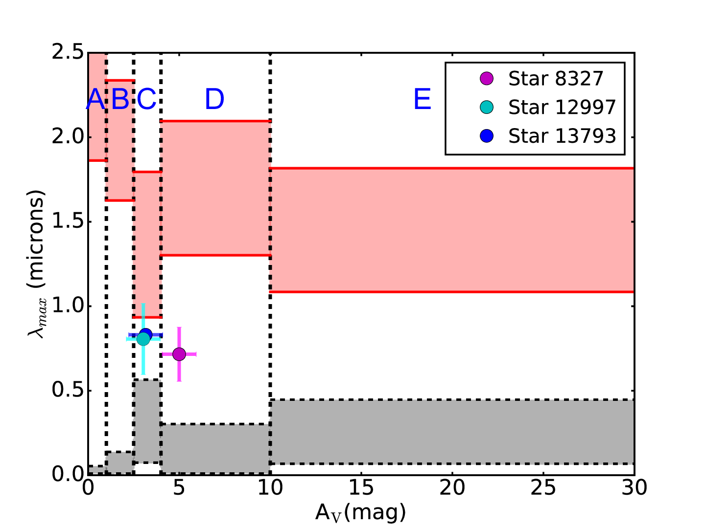
Similarly, we plotted versus in Figure 16 to trace the variation of the polarization spectrum in the infrared. The data were separated into five groups, in a fashion similar to Figure 13 (, 1.0–2.5, 2.5–4.0, 4.0–10.0, and 10.0 mag, labelled as A, B, C, D, and E, respectively). The statistical properties of for these groups are listed in Table 4. The average changes significantly with , with the greatest value being found in group B.
The values of converted from were listed in Table 4. The range of derived from the group averaged was 1.46–1.93 m, significantly higher than the 0.73–0.78 m range derived from . The inconsistency implies that the Serkowski relation may not well describe the polarization spectrum at near-infrared wavelengths. Martin [53] suggested that the near-infrared polarization spectrum can be better described by a power-law
| (6) |
where 1.6–2.0. In the infrared, polarization color can still constrain the power-law index by
| (7) |
The derived from our data are listed in Table 4. These indices probably vary with and have a peak at 2.5–4 mag, as shown by Figure 16. Kim & Martin [44] showed that the index could depend on the amount of micron-size dust grains. Our results hint that the population of micron-size dust grains might evolve with , and a significant change occurs at of 2.5–4 mag.
V DISCUSSION
V.1 Evolution of Dust Grains
The derived values obtained in previous studies [79, 83, e.g.,] are expected to be related to the small-size cutoff of the grain size distribution. Whittet & van Breda [79] found that is related to the ratio of total to selective extinction () by an empirical relation , tracing the reddening changes with grain size distribution changes. However, with more observations, Andersson & Potter [3] found no correlation between and for individual clouds; the empirical relation could only be recovered by combining the data for all of their observed clouds. They further argued that may depend on both grain size distributions and dust alignment conditions.
Whittet et al. [82] showed, in their RATs simulations with constant grain size distribution, that increases with because small dust grains become less aligned due to the decaying and reddening of the external radiation field by extinction. Their model predicts a smooth increase of from 0.45 to 0.75 m as increases from 0 to 6 mag. However, our derived values, 0.73–0.78 m, do not significantly change with . In addition, our data show significant decrease of the intrinsic dispersion of from 0.110.08 (1.0–2.5 mag) to 0.07 (2.5–4.0 mag) possibly due to changes of the grain size distribution.
The change in the dispersion of implies that the grain size distribution in the dense regions could be more uniform than in the diffuse regions. We speculate that the difference is due to the evolution of dust grain size. In grain-grain collision models [40, 35, 58], the grain size distributions are expected to be modified by the competing effects of fragmentation and coagulation. Steady-state grain size distributions are eventually reached when these two effects achieve equilibrium. As a result, the apparent uniform grain size distribution in the dense regions may hint at the existence of stabilized grain-grain collision processes. Together with the increase of , this non-evolution of grains in the dense regions favors the notion that grain growth has already taken place before reaches 2.5-4.0 mag.
In Figure 17, we show that the derived from a Serkowski relation based on analysis of yielded an average of 1.46–1.93 m. This was inconsistent with derived from , which yielded an average of 0.73–0.78 m. To reach a of 0.73–0.78 m, would need to be 2.3, which is much higher than the observed range of mean values from 0.960.28 to 1.710.21. This indicates that at least the measured -band infrared polarization exceeds the predictions of the Serkowski relation. This excess infrared polarization was also found in early studies [54, 57, 38, e.g.,], and is better fit by a power-law (Equation 7). We found that a power-law with ranging from to can explain our data for different . The index appears to vary with , and has its highest value for 2.5–4.0 mag. Our are similar to, or smaller than, the value of measured toward ScO-Oph and CyG OB2 [55], and measured toward the Galactic center [30].
Two models have tried to explain the physical origin of the excess infrared polarization over the Serkowski relation. Kim & Martin [44] showed that a model with a dust grain mixture with sizes of 0.3 m and 0.6–1 m can reproduce the observational Serkowski relation while also exhibiting a power-law excess infrared polarization. Li & Greenberg [49] showed that an organic refractory mantled dust grain model with a Gaussian grain size distribution could reproduce the observed excess infrared polarization without requiring a high abundance of micron-size dust grains. Our results show that the observed power-law index might vary with , providing new constraints for future models.
V.2 How Deep Into a Cloud Can Polarization Be Used to Reveal B-fields?
Polarization efficiency has been used to indicate how deep into a cloud, in , the dust grains remain aligned. Goodman et al. [27] found a PE- power-law index of in L1755 in the JHK bands. This constancy of P with was used to argue that near-infrared polarization does not trace the B-field within dense clouds. In contrast, Whittet et al. [82] found an index of in Taurus at -band, showing that polarization can trace the B-field, at least up to mag.
The power-law PE versus indices characterizing these two cases can be found in our data, but for different ranges. The power index of measured for -band in low regions is similar to the results found in L1755 at -band [27] for 8–10 mag . Our index of for -band is close to the value found in Taurus at -band () by Whittet et al. [82] and the value found in numerous starless cores at -band () for 20 mag by Jones et al. [42]. In addition, the intermediate index found in the -band is similar to the results found in Pipe-109 using -band (, Alves et al. 2) and in L204 using -band (, Cashman & Clemens 8). We found our steepest index, of , in the -band and our softest index, of , in the -band in high regions.
The softer indices of to are only found in high regions in - and -bands, while a variety of steeper indices are found in low regions. The indices match predictions of RATs models with constant grain size distributions [82]. The same models predicts a steepening of PE as approaches 10 mag, due to the strong extinction of external radiation. Here, however, the indices we measure for high regions show that the dust with up to 20 mag still contributes to the measured polarization: the polarization efficiency at mag is only a factor of 2 lower than that at 4 mag. Thus, the notion that only the dust on the surfaces of clouds is aligned, as concluded by Goodman et al. [27], is not supported here.
V.3 The Diverse PE in Low Regions
It is interesting that a variety of PE versus power-law behaviors are seen across the IC5146 cloud system. We showed that the indices derived using -band varied with region location in Figure 11. The diverse PE- relations likely depend more on and region choice and less on wavelength, as the indices derived from - and -bands in the same region are almost the same. If all the stellar values from all of the low regions are combined into a single plot and fitted, the location dependence of the PE- relation would be mixed and thereby lost. The index of derived from -band using all data with low is merely the average from the mixed PE- relation shown in Figure 11. This is different from the suggestion by Goodman et al. [27] that the power-law index of -1 indicates that starlight polarization only traces the dust grains on the surfaces of clouds.
Three possibilities could explain the origin of the wide variation of the PE- relation.
i) The grain size distributions could be diverse and vary greatly from region to region for low . In Section IV.3, we showed that the dispersion of , estimated from , is significantly larger for mag, suggesting that grain size distributions are diverse. This diversity is likely region-dependent, since the different values were derived from different sightlines. The grain size distribution is a key element of the RATs theory; radiation can efficiently align dust grains having sizes comparable to its wavelength, and wavelength determines radiation penetration ability.
ii) Depolarization effects may occur if multiple polarizing layers exist. In Figure 11, we showed that the PE vs indices derived in the western part of IC5146 cloud were steeper than , hence the polarization percentage must decrease with . This may be a result of depolarization. If a multiple layer structure, with the layers having different B-field orientations, exists along a line of sight, the net transferred polarization from the different layers would be reduced. Arzoumanian et al. [5] found rich and hierarchical filamentary structure in the IC5146 cloud system. These filaments can naturally produce a multiple layer structure if the projections of such structures overlap along the line of sight. In addition, they further found that most of the filaments in the western part of the IC5146 cloud system were supercritical, which might twist to cause complex B-fields. This could explain the steeper indices found in the western part of the cloud.
iii) The degree of dust alignment may be affected by one or more bright illuminators, such as the stars in the Cocoon Nebula. Cashman & Clemens [8] found a possible dependence of PE- index for regions in the L204 cloud 3 with distance from a nearby illuminator. Brighter stellar radiation can boost alignment of the dust, and the alignment efficiency will mainly depend on the optical depth to the illuminator. In IC5146, the Cocoon Nebula stellar cluster could be a strong illuminator that is able to affect grain alignment. However, the radiation from the Cocoon Nebula is also highly shadowed by the main filament structure, making the optical depth from the Cocoon Nebula to the other regions difficult to estimate.
V.4 The Breakpoint in PE- Relations
In Section IV.2, we showed that PE decays with and a breakpoint (BP) of mag separates two different power-law slopes of in -band. Breakpoints of PE near –3 mag are rarely seen. Pipe-109 shows a breakpoint at 9.5 mag with power index changing from -1.00 to -0.34 [2]. LDN 183 shows a breakpoint at mag with power index changing from -0.6 to -1 [19, 14, 4]. Jones et al. [42] also found a break point at mag with power index changing from -0.5 to -1 toward several starless cores. Jones et al. [43] found an break point at very high , hundreds mag, in the Class 0 YSO G034.43+00.24 MM1 with a change of power index from -1 to -0.5.
Three mechanisms could change the power-law indices with , though in opposite directions. Radiation into the deepest regions could be too faint to align the dust grains, so the power-law index for high regions should steepen [82]. But, if grains grow at higher , the alignment efficiency will be higher for dust with size comparable to the wavelength [48], hence the power-law index will become flatter in the dense regions where only radiation with longer wavelengths can penetrate and the dust grains are believed to grow. In addition to the change of dust properties, internal radiation fields from embedded sources within dense clouds could also enhance dust alignment, and flatten the power-law index.
Andersson et al. [4] suggest that the origin of the breakpoint found in LDN 183 is likely due to the extinction of external radiation, because their power-law index in low regions, of -0.6, is consistent with prediction of the RATs model assuming constant grain size [82]. Similar trends were also found within several starless cores by Jones et al. [42], and they further showed that the RATs theory can explain the break point of mag, where the dust optical depth, for the wavelength comparable to the maximum grain size, becomes optically thick.
Our results showed an opposite trend as compared to the case of LDN183: steeper indices ranging from -0.71 to -1.23 were found in low regions while flatter indices ranging from -0.25 to -0.53, consistent with the Whittet et al. [82] model, were found in high regions, for all observed wavebands. The results from Alves et al. [2] toward the Pipe-109 and Jones et al. [43] in G034.43+00.24 MM1 show similar trends as ours, but with different breakpoints. The flattened slopes in high regions more likely originate from efficient grain alignment due to either grain growth or internal radiation fields. Because Pipe-109 is a starless object but G034.43+00.24 MM1 is a Class 0 YSO, the change of slope for the former likely results mainly from grain growth while internal radiation might play an important role in the latter. Since the breakpoint of 2.8 mag shown in our data is consistent with the of the regions where the intrinsic dispersion of drops significantly (=2.5–4.0 mag), our observed trend is more likely caused by grain growth.
An open question is why the breakpoint we measure is so different from the 9.5 mag value in Alves et al. [2], although both breakpoints likely result from grain growth. The difference could originate from two possible reasons. First, Alves et al. [2] lacked samples in low regions, and thus a broken power-law with breakpoint at mag would be difficult to identify. Second, the difference may come from different grain growth conditions. Ormel et al. [58] simulated the evolution of dust grain size, based on grain-grain collisions. They found that dust grains with ice-coatings are more likely to aggregate and grow than are grains without ice-coatings, due to the increased surface stickiness. Chiar et al. [10] found that -ice in IC5146 only exists in regions exhibiting extinctions exceeding 4 mag, a value quite similar to the breakpoint we found. Thus, H2O-ice mantling could induce a breakpoint via enhanced grain growth. Similarly, Whittet et al. [81] found the observed in Taurus changed from 3 to 4 around 3.2 mag, coincident with the extinction threshold for H2O-ice mantling in Taurus, and suggest that mantle growth is an important process in initial grain growth. We conclude that such mantling also enables greater efficiency of dust grain alignment, permitting magnetic field to be traced deeper into clouds than if such mantling is not present.
VI CONCLUSIONS
We performed optical and infrared polarimetry observations toward background stars seen through the IC5146 dark cloud system using AIMPOL at the ARIES Observatory, TRIPOL at the Lulin Observatory, and Mimir at the Lowell Observatory Perkins Telescope. A total of 2022 stars showed significant polarization detection in at least one of the four wavebands observed. From analysis of these data, we found:
- 1.
Polarization efficiency (PE ) decreases with as a power-law or broken power-law. The values of the power-law indices likely depend more on the choice of targeted regions and local extinction, and less on observing wavelength.
- 2.
A cloud averaged power-law index of for PE vs. was found in -band for low , the same as the index found in L1755 by Goodman et al. [27]. However, we showed that the index of resulted from the admixture of a variety of PE- relations, whose local-regional indices varied from -0.8 to -1.8, different from the suggestion by Goodman et al. [27] that the index of -1 indicates that background starlight polarization only traces the dust grains on the surface of clouds.
- 3.
A broken power-law relation for PE vs. in -band exhibits a breakpoint at about 2–3 mag. The power-law index in high regions is shallow and consistent with predictions from RATs models [82], while the indices in low regions are steeper and vary with region. The shallow index in high regions is likely due to grain growth.
- 4.
Excess infrared polarization, over that predicted by the Serkowski relation, was observed in , possibly resulted from abundance enhancements of large, micron-size dust grains. The average varies with from 0.960.20 to 1.710.21, and exhibits its highest value of 1.710.21 for in the 2.5–4.0 mag range. This implies that the abundance of such micron-size dust grains might change with .
- 5.
Polarization color () is a useful tool to constrain , the peak of the Serkowski relation, which may trace the small-size cutoff of the grain size distribution. We found both the average and dispersion of decreased from the 1.0 2.5 mag range to the 2.5 4.0 mag range. These variations suggest that the small-size cutoffs of grain size distributions are most likely due to efficient grain-grain collisions, and thus hint that grain growth could already take place by 2.5–4.0 mag, possibly enhanced at this relatively low range by the presence of ice mantles on the grains.
In conclusion, this study revealed that dust grains in the diffuse molecular regions ( mag) of the IC5146 dark cloud system have diverse size distributions. As approaches mag, sub-micron dust grains grow significantly due to grain-grain collisions. The size distributions may also become more uniform as increases as a balance is reached between fragmentation and coagulation. In addition, the larger, micron-sized grains likely already exist in the diffuse regions, and their abundances and sizes likely change with . In the next paper of this series, we will use these polarization data to characterize the magnetic field morphology and strength across this system of filamentary dark molecular clouds associated with IC5146.
ccccccccccccccccBccccccccccccccccccBccccccccccccc
-band Polarimetry -band Polarimetry -band Polarimetry -band Polarimetry 2MASS Catalog WISE Catalog
ID R.A. Dec. J H K W1 W2 aaThe uncertainties of are 0.93 mag, estimated in Section 3.1 UF
(deg) (deg) (%) (%) (%) (%) (%) (%) (deg) (deg) (%) (%) (%) (%) (%) (%) (deg) (deg) (%) (%) (%) (%) (%) (%) (deg) (deg) (%) (%) (%) (%) (%) (%) (deg) (deg) (mag) (mag) (mag) (mag) (mag) (mag) (mag) (mag) (mag) (mag) (mag)
(1) (2) (3) (4) (5) (6) (7) (8) (9) (10) (11) (12) (13) (14) (15) (16) (17) (18) (19) (20) (21) (22) (23) (24) (25) (26) (27) (28) (29) (30) (31) (32) (33) (34) (35) (36) (37) (38) (39) (40) (41) (42) (43) (44) (45) (46) (47)
8327 326.3935 47.6311 1.68 0.32 1.94 0.33 2.54 0.34 24.51 3.44 1.59 0.07 2.18 0.07 2.70 0.07 26.90 0.70 0.41 0.11 0.65 0.11 0.76 0.11 28.62 4.28 0.03 0.22 0.53 0.20 0.49 0.20 43.34 11.76 10.861 0.019 9.727 0.028 9.352 0.017 9.163 0.023 9.314 0.019 5.00 1
12997 326.6920 47.4848 0.98 0.24 0.90 0.24 1.31 0.25 21.34 4.86 0.54 0.05 1.40 0.05 1.50 0.05 34.46 0.97 0.47 0.23 0.47 0.22 0.62 0.23 22.28 10.49 0.31 0.25 0.44 0.16 0.51 0.20 27.36 11.20 11.483 0.025 10.745 0.03 10.462 0.023 10.257 0.022 10.35 0.021 3.03 1
13793 326.7371 47.4965 2.11 0.18 1.40 0.18 2.53 0.18 16.75 1.97 2.16 0.05 1.75 0.05 2.78 0.05 19.55 0.50 0.98 0.21 0.70 0.23 1.19 0.22 17.82 5.33 0.37 0.24 0.36 0.13 0.48 0.19 21.98 11.66 11.205 0.023 10.333 0.028 10.075 0.022 9.894 0.022 9.961 0.021 3.16 1
| Band | F-value | p-value | AICc | AICc | Preferred Model |
|---|---|---|---|---|---|
| (model 1 model 2) | (model 1) | (model 2) | |||
| 0.30 | 0.75 | 22.30 | 30.00 | ||
| i’ | 0.40 | 0.68 | -5.64 | 5.74 | |
| H | 3.95 | 0.04 | 40.68 | 39.92 | |
| K | 1.13 | 0.36 | 8.90 | 14.57 | |
Note. — This table is available in its entirety in a machine-readable form in the online journal. A portion is shown here for guidance regarding its form and content.
Note. — The preferred model is determined if (1) the p value from F-test is below 0.05 (95% confidence level) or (2) the model has lower AICc value
| Group | range | Mean | STD | Intrinsic | aaThe calculated from the mean . Uncertainties were calculated from the means and the propagated uncertainties of the means, assuming c=2.3. | |
|---|---|---|---|---|---|---|
| (mag) | DispersionbbThe intrinsic dispersions and the uncertainties of the dispersions. The intrinsic dispersion cannot be defined if the observed dispersion is less than instrumental uncertainty. | (m) | ||||
| A | -2.0–1.0 | 0.53 | ||||
| B | 1.0–2.5 | 0.97 | ||||
| C | 2.5–4.0 | 0.80 | … | |||
| D | 4.0 | 0.78 | ||||
| Group | range | Mean | STD | Intrinsic | aaThe calculated from the mean . Uncertainties were calculated from the means and the propagated uncertainties of the means, assuming c=2.3. | Power-law index | |
|---|---|---|---|---|---|---|---|
| (mag) | DispersionbbThe intrinsic dispersions and the uncertainties of the dispersions. The intrinsic dispersion cannot be defined if the observed dispersion is less than instrumental uncertainty. | (m) | |||||
| A | -2.0–1.0 | 0.660.12 | 0.390.21 | 0.31 | 0.270.30 | ||
| B | 1.0–2.5 | 0.960.20 | 0.420.31 | 0.52 | … | ||
| C | 2.5–4.0 | 1.710.21 | 0.570.24 | 0.72 | … | ||
| D | 4.0–10.0 | 1.310.13 | 0.540.20 | 0.54 | … | ||
| E | 10.0 | 1.630.16 | 0.510.19 | 0.58 | … | ||


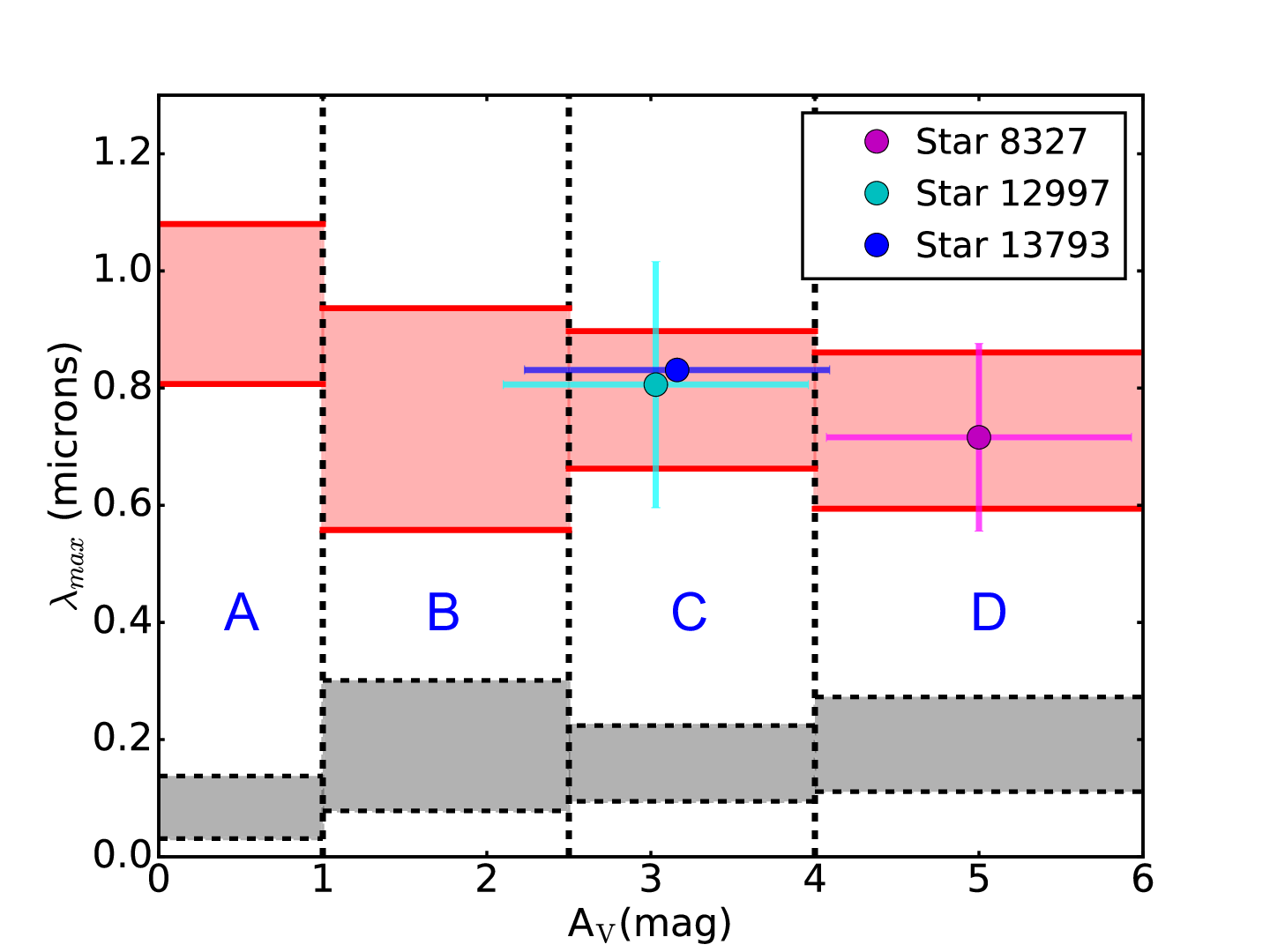
. The red and grey sets of zones identify the two degenerate sets of solutions to the Serkowski relation. The three stars whose four-band polarimetry data were fitted to the Serkowski relation (see Figure 12) are plotted as filled, colored circles with error bars and are consistent with the set of red zone solutions corresponding to greater values of .

References
- [1] Akaike, H. 1974, IEEE Transactions on Automatic Control, 19, 716
- [2] Alves, F., Frau, P., Girart, J. M., et al. 2014, A&A, 569,
- [3] Andersson, B.-G., & Potter, S. B. 2007, ApJ, 665, 369
- [4] Andersson, B.-G., Lazarian, A., & Vaillancourt, J. E. 2015, ARA&A, 53, 501
- [5] Arzoumanian, D., André, P., Didelon, P., et al. 2011, A&A, 529, L6
- [6] Astropy Collaboration, Robitaille, T. P., Tollerud, E. J., et al. 2013, A&A, 558, A33
- [7] Bertin, E., & Arnouts, S. 1996, A&AS, 117, 393
- [8] Cashman, L. R., & Clemens, D. P. 2014, ApJ, 793, 126
- [9] Chapman, N. L., Goldsmith, P. F., Pineda, J. L., et al. 2011, ApJ, 741, 21
- [10] Chiar, J. E., Pendleton, Y. J., Allamandola, L. J., et al. 2011, ApJ, 731, 9
- [11] Cho, J., & Lazarian, A. 2005, ApJ, 631, 361
- [12] Clayton, G. C., Anderson, C. M., Magalhaes, A. M., et al. 1992, ApJ, 385, L53
- [13] Clemens, D. P., Sarcia, D., Grabau, A., et al. 2007, PASP, 119, 1385
- [14] Clemens, D. P. 2012, ApJ, 748, 18
- [15] Clemens, D. P., Pinnick, A. F., Pavel, M. D., Taylor, B. W., 2012a, ApJS, 200, 19
- [16] Clemens, D. P., Pinnick, A. F., & Pavel, M. D. 2012b, ApJS, 200, 20
- [17] Clemens, D. P., Pavel, M. D., & Cashman, L. R. 2012c, ApJS, 200, 21
- [18] Clemens, D. P., Tassis, K., & Goldsmith, P. F. 2016, ApJ, 833, 176
- [19] Crutcher, R. M. 2004, Ap&SS, 292, 225
- [20] Davis, L., Jr., & Greenstein, J. L. 1951, ApJ, 114, 206
- [21] Dolginov, A. Z., & Mitrofanov, I. G. 1976, Ap&SS, 43, 291
- [22] Draine, B. T., & Weingartner, J. C. 1996, ApJ, 470, 551
- [23] Draine, B. T., & Weingartner, J. C. 1997, ApJ, 480, 633
- [24] Eswaraiah, C., Pandey, A. K., Maheswar, G., et al. 2011, MNRAS, 411, 1418
- [25] Eswaraiah, C., Pandey, A. K., Maheswar, G., et al. 2012, MNRAS, 419, 2587
- [26] Fisher R. A., 1925, Nat, 123, 866
- [27] Goodman, A. A., Jones, T. J. B., Lada, E. A. , & Myers, P. C. 1995, ApJ, 448, 748
- [28] Griffin, M.J., Abergel, A., Abreu, A., et al. 2010, Å, 518, L3
- [29] Hall, J. S. 1949, Sci, 109, 166
- [30] Hatano, H., Nishiyama, S., Kurita, M., et al. 2013, AJ, 145, 105
- [31] Heiles, C. 2000, AJ, 119, 923
- [32] Herbig, G. H., & Dahm, S. E. 2002, AJ, 123, 304
- [33] Hiltner, W. A. 1949a, ApJ, 109, 471
- [34] Hiltner, W. A. 1949b, Sci, 109, 165
- [35] Hirashita, H., & Yan, H. 2009, MNRAS, 394, 1061
- [36] Hoang, T., & Lazarian, A. 2009, ApJ, 695, 1457
- [37] Indebetouw, R., Mathis, J. S., Babler, B. L., et al. 2005, ApJ, 619, 931
- [38] Jones, T. J. 1990, AJ, 99, 1894
- [39] Jones, R. V., & Spitzer, L., Jr. 1967, ApJ, 147, 943
- [40] Jones, A. P., Tielens, A. G. G. M., & Hollenbach, D. J. 1996, ApJ, 469, 740
- [41] Jones, E., Oliphant, E., Peterson, P., et al. 2001, http://www.scipy.org/
- [42] Jones, T. J., Bagley, M., Krejny, M., Andersson, B.-G., & Bastien, P. 2015, AJ, 149, 31
- [43] Jones, T. J., Gordon, M., Shenoy, D., et al. 2016, AJ, 151, 156
- [44] Kim, S.-H., & Martin, P. G. 1995, ApJ, 444, 293
- [45] Lada, C. J., Lada, E. A., Clemens, D. P., & Bally, J. 1994, ApJ, 429, 694
- [46] Lada, C. J., Alves, J., & Lada, E. A. 1999, ApJ, 512, 250
- [47] Lazarian, A., Goodman, A. A., & Myers, P. C. 1997, ApJ, 490, 273
- [48] Lazarian, A., & Hoang, T. 2007, MNRAS, 378, 910
- [49] Li, A., & Greenberg, J. M. 1997, A&A, 323, 566
- [50] Li, H.-b., Fang, M., Henning, T., & Kainulainen, J. 2013, MNRAS, 436, 3707
- [51] Lombardi, M., & Alves, J. 2001, A&A, 377, 1023
- [52] Ludden, Thomas M., Beal, Stuart L., & Sheiner, Lewis B, C. 1994, Journal of Pharmacokinetics and Biopharmaceutics, 22, 5, 431
- [53] Martin, P. 1989, Interstellar Dust, 135, 55
- [54] Martin, P. G., & Whittet, D. C. B. 1990, ApJ, 357, 113
- [55] Martin, P. G., Adamson, A. J., Whittet, D. C. B., et al. 1992, ApJ, 392, 691
- [56] Meingast, S., Lombardi, M., & Alves, J. 2017, A&A, 601, A137
- [57] Nagata, T. 1990, ApJ, 348, L13
- [58] Ormel, C. W., Paszun, D., Dominik, C., & Tielens, A. G. G. M. 2009, A&A, 502, 845
- [59] Parzen, E. 1962, Ann. Math. Statist., 33, 1065
- [60] Planck Collaboration, Ade, P. A. R., Aghanim, N., et al. 2016, A&A, 586, A138
- [61] Purcell, E. M. 1979, ApJ, 231, 404
- [62] Rautela, B. S., Joshi, G. C., & Pandey, J. C., 2004, Bull. Astron. Soc. India, 32, 159
- [63] Robitaille, T., & Bressert, E. 2012, Astrophysics Source Code Library, ascl:1208.017
- [64] Rosenblatt, M. 1956, Ann. Math. Statist., 27, 832
- [65] Sato, S., T. Zenno, T. Nagayama, et al., APRIM 2011, NARIT Conference Series, 1, 413
- [66] Sato, S., T. Zenno, T. Nagayama, et al., 2017, submitted to PASJ
- [67] Serkowski, K. 1973, Interstellar Dust and Related Topics, 52, 145
- [68] Serkowski, K., Mathewson, D. S., & Ford, V. L. 1975, ApJ, 196, 261
- [69] Schaefer, B., Collett, E., Smyth, R., et al. Am. J. Phys. 75, 163 (2007).
- [70] Schmidt, G. D., Elston, R., & Lupie, O. L., 1992, AJ, 104, 1563
- [71] Skrutskie, M. F., Cutri, R. M., Stiening, R., et al. 2006, AJ, 131, 1163
- [72] Sugitani, K., Nakamura, F., Watanabe, M., et al. 2011, ApJ, 734, 63
- [73] Sugiura, N. 1978, Comm. Statist., A7, 13
- [74] van der Walt, S., Colbert, S. C., & Varoquaux, G. 2011, “The NumPy array: A structure for efficient numerical computation,” Comput. Sci. Eng. 13(2), 22–30
- [75] van Leeuwen, F. 2007, A&A, 474, 653
- [76] Voshchinnikov, N. V., Das, H. K., Yakovlev, I. S., & Il’in, V. B. 2013, Astronomy Letters, 39, 421
- [77] Voshchinnikov, N. V., & Hirashita, H. 2014, MNRAS, 445, 301
- [78] Wardle, J. F. C., & Kronberg, P. P. 1974, ApJ, 194, 249
- [79] Whittet, D. C. B., & van Breda, I. G. 1978, A&A, 66, 57
- [80] Whittet, D. C. B., Martin, P. G., Hough, J. H., et al. 1992, ApJ, 386, 562
- [81] Whittet, D. C. B., Gerakines, P. A., Hough, J. H., & Shenoy, S. S. 2001, ApJ, 547, 872
- [82] Whittet, D. C. B., Hough, J. H., Lazarian, A., & Hoang, T. 2008, ApJ, 674, 304
- [83] Wilking, B. A., Lebofsky, M. J., & Rieke, G. H. 1982, AJ, 87, 695
- [84] Wright, E. L., Eisenhardt, P. R. M., Mainzer, A. K., et al. 2010, AJ, 140, 1868-1881