Admissible multi-arm stepped-wedge cluster randomized trial designs

We designate a MA-SW as any trial conforming to the following requirements

• •

  The trial is carried out in $C\geq 2$ clusters, over $T\geq 2$ time periods, with $m>1$ measurements made in each cluster in each time period;

• •

  In each time period, each cluster receives a combination of a set of $D$ interventions (indexed by $d=0,\dots,D-1$);

• •

  The sequence of intervention allocations for each cluster is specified randomly.

We make no assumptions about whether the $m$ measurements from each time period are on different patients; a cross-sectional design, or the same patients; a cohort design. We do not require each cluster to begin on, receive, or conclude the trial on any particular intervention. We also do not enforce the usual one-directional switching associated with conventional SW-CRTs, so as to allow for transitions between experimental interventions in any order, if this is desired. As a consequence of this, the methodology we describe is applicable to the design of multi-arm cluster randomized crossover trials. We keep in mind, however, that each of the interventions must be received by at least one cluster in some time period for its effect to be estimable.

Throughout we assume that the accrued data from the trial will be normally distributed, and an identifiable linear mixed model will be utilized for data analysis, denoted as

$$\boldsymbol{y}=A\boldsymbol{\beta}+Z\boldsymbol{u}+\boldsymbol{\epsilon},$$

where

• •

  $\boldsymbol{y}$ is the vector of responses;

• •

  $\boldsymbol{\beta}=(\beta_{1},\dots,\beta_{p})^{\top}$ is a vector of $p$ fixed effects;

• •

  $A$ is the design matrix which links $\boldsymbol{y}$ to $\boldsymbol{\beta}$;

• •

  $\boldsymbol{u}$ is a vector of random effects, with $\boldsymbol{u}\sim N(\boldsymbol{0},G)$, where $G$ is a specified (assumed known) matrix;

• •

  $Z$ is the design matrix which links $\boldsymbol{y}$ to $\boldsymbol{u}$;

• •

  $\boldsymbol{\epsilon}$ is a vector of residuals, with $\boldsymbol{\epsilon}\sim N(\boldsymbol{0},R)$, where $R$ is a specified (assumed known) matrix.

We suppose that $\boldsymbol{\beta}$ has been specified such that its first $q$, $q\leq p$, elements, $(\beta_{1},\dots,\beta_{q})^{\top}$, are our parameters of interest. Typically, we may have that $q=D-1$, with these parameters representing either the direct effects of a set of experimental interventions relative to some control, or the direct effect of intervention arm $d$ relative to intervention arm $d-1$, for $d=1,\dots,D-1$. However, we do not require that this be the case. Then, we assume that we will test the following one-sided hypotheses

$$H_{0f}:\beta_{f}\leq 0,\qquad H_{1f}:\beta_{f}>0,\qquad f=1,\dots,q.$$

We note though that the determination of MA-SW designs for alternative hypotheses of interest, e.g., two-sided hypotheses, is also easily achievable by adapting what follows.

To test these hypotheses, following trial completion, we estimate $\boldsymbol{\beta}$ using the maximum likelihood estimator of a linear mixed model

$$\hat{\boldsymbol{\beta}}=(\hat{\beta}_{1},\dots,\hat{\beta}_{p})^{\top}=\{A(ZGZ^{\top}+R)^{-1}A\}^{-1}A^{\top}(ZGZ^{\top}+R)^{-1}\boldsymbol{y}.$$

Then

$$\text{cov}(\hat{\boldsymbol{\beta}},\hat{\boldsymbol{\beta}})=\Lambda=\{A(ZGZ^{\top}+R)^{-1}A\}^{-1}.$$

We set $\hat{\boldsymbol{\beta}}_{q}=(\hat{\beta}_{1},\dots,\hat{\beta}_{q})^{\top}$, and denote the covariance matrix of $\hat{\boldsymbol{\beta}}_{q}$ by $\Lambda_{q}$. That is, $\text{cov}(\hat{\boldsymbol{\beta}}_{q},\hat{\boldsymbol{\beta}}_{q})=\Lambda_{q}$.

Our conclusions are then based upon the following Wald test statistics

$$Z_{f}=\frac{\hat{\beta}_{f}}{\sqrt{\text{var}(\hat{\beta}_{f})}}=\hat{\beta}_{f}\Lambda^{-1/2}_{[f,f]}=\hat{\beta}_{f}I_{f}^{1/2},\qquad f=1,\dots,q.$$

Explicitly, we reject $H_{0f}$ if $Z_{f}>e$, for critical boundary $e$. Given $e$, we can determine for any vector of true fixed effects $\boldsymbol{\beta}_{q}$ the probability each particular $H_{0f}$ is rejected, and the probability we reject at least one of $H_{01},\dots,H_{0q}$, via the following integrals

	$\displaystyle\mathbb{P}(\text{Reject }H_{0f}\mid\beta_{f})$	$\displaystyle=\int_{e}^{\infty}\phi(x,\beta_{f}I_{f}^{1/2},1)\mathrm{d}x,$
	$\displaystyle\mathbb{P}(\text{Reject at least one of }H_{01},\dots,H_{0q}\mid\boldsymbol{\beta}_{q})$	$\displaystyle=1-\int_{-\infty}^{e}\dots\int_{-\infty}^{e}\phi\{\boldsymbol{x},\boldsymbol{\beta}_{q}\circ\boldsymbol{I}^{1/2},\text{diag}(\boldsymbol{I}^{1/2})\Lambda_{q}\text{diag}(\boldsymbol{I}^{1/2})\}\mathrm{d}x_{q}\dots\mathrm{d}x_{1}.$

Here

• •

  $\phi(\boldsymbol{x},\boldsymbol{\mu},\Sigma)$ is the probability density function of a multivariate normal distribution with mean $\boldsymbol{\mu}=(\mu_{1},\dots,\mu_{k})^{\top}$ and covariance matrix $\Sigma$, $\text{dim}(\Sigma)=k\times k$, evaluated at vector $\boldsymbol{x}=(x_{1},\dots,x_{k})^{\top}$;

• •

  $(a_{1},\dots,a_{n})^{\top}\circ(b_{1},\dots,b_{n})^{\top}=(a_{1}b_{1},\dots,a_{n}b_{n})^{\top}$;

• •

  $\boldsymbol{I}^{1/2}=(I_{1}^{1/2},\dots,I_{q}^{1/2})^{\top}$ is the element-wise square root of the vector of information levels for $\boldsymbol{\beta}_{q}$;

• •

  $\text{diag}(\boldsymbol{v})$ for a vector $\boldsymbol{v}$ indicates the matrix formed by placing the elements of $\boldsymbol{v}$ along the leading diagonal.

Determining an appropriate value for $e$ depends upon whether a correction for multiple testing is to be utilized. Without such a correction, $e$ can be chosen to control the per-hypothesis error-rate to $\alpha$ by setting $e$ as the solution to

$$\alpha=\int_{e}^{\infty}\phi(x,0,1)\mathrm{d}x.$$

Alternatively, the familywise error-rate, the probability of one or more false rejections, can be controlled for example using the Bonferroni correction, which sets in this instance $e$ to be the solution of

$$\frac{\alpha}{q}=\int_{e}^{\infty}\phi(x,0,1)\mathrm{d}x.$$

The choice of whether to utilize a multiple testing correction is not a simple one, with much debate in the literature around when it is necessary. It seems reasonable for MA-SWs however to extrapolate from previous discussions, and note that one should correct in confirmatory settings, but should not always feel the need to in exploratory settings.[30]

The above fully specifies a hypothesis testing procedure for a MA-SW. However, at the design stage, it is important to be able to determine values of $m$, $C$, and $T$ that provide both the desired per-hypothesis or familywise error-rate, and the desired power. Here, we describe two types of power that could be required, since power is not a simple concept in multi-arm trials.

We suppose that power of at least $1-\beta$ is required either to reject each $H_{0f}$ (individual power), or at least one of $H_{01},\dots,H_{0q}$ (combined power), when $\boldsymbol{\beta}_{q}=\boldsymbol{\delta}=(\delta_{1},\dots,\delta_{q})^{\top}$. The element $\delta_{f}$ here represents a clinically relevant difference for the effect $\beta_{f}$. Using our notation from earlier, these requirements can be written as

	$\displaystyle\min_{f\in\{1,\dots,q\}}\mathbb{P}(\text{Reject }H_{0f}\mid\delta_{f})$	$\displaystyle\geq 1-\beta,$
	$\displaystyle\mathbb{P}(\text{Reject at least one of }H_{01},\dots,H_{0q}\mid\boldsymbol{\delta})$	$\displaystyle\geq 1-\beta.$

The choice between these requirements should be made based on several considerations. The latter will likely require smaller sample sizes, however it would leave a trial less likely to reject all false null hypotheses. Therefore, trialists must weigh up the cost restrictions and goals of their trial.

We can now return to our considerations on determining appropriate values for $m$, $C$, and $T$. We must also determine as part of the same process a matrix $X$ that indicates the planned allocation of interventions to each cluster across the time periods. Extending the notation commonly utilised for SW-CRTs, $X$ is a $C\times T$ matrix, with $X_{ij}$ indicating which intervention(s) cluster $i$ receives in time period $j$. If only a single intervention is given to each cluster in each time period, then $X_{ij}$ will be a single number. Otherwise, it may be some combination of values, indicating allocation to multiple interventions. With this, it will now be useful to denote the design utilized by a trial by $\mathscr{D}=\{m,C,T,X\}$, and the associated covariance matrix for $\boldsymbol{\beta}_{q}$ by $\Lambda_{\mathscr{D}}$. Our goal is then to optimize $\mathscr{D}$.

Most of the work on sample size determination for SW-CRTs pre-supposes that two of the three parameters $m$, $C$, and $T$ are fixed (with one usually $T$), and then looks to identify the third. In addition, the matrix $X$ is usually specified, if not explicitly (in the case where $C$ and $T$ are fixed), then through some rule such as balanced stepping. Here, we take an alternate approach to the determination of the preferred design. We assume that a set of allowed values for $T$ has been specified, $\mathfrak{T}=\{T_{1},\dots,T_{|\mathfrak{T}|}\}$. We then suppose that sets of allowed values for $C$, for each element of $\mathfrak{T}$, have been specified. We denote these by $\mathfrak{C}=\{\mathfrak{C}_{T_{1}},\dots,\mathfrak{C}_{T_{|\mathfrak{T}|}}\}$, with $\mathfrak{C}_{T_{i}}=\{C_{1},\dots,C_{|\mathfrak{C}_{T_{i}}|}\}$. Furthermore, we suppose that for each allowed $C$,$T$ combination, a set of allowed values for $m$ have been provided; $\mathfrak{M}_{C,T}=\{m_{1},\dots,m_{|\mathfrak{M}_{C,T}|}\}$. We then take $\mathfrak{M}=\{\mathfrak{M}_{C,T}:T\in\mathfrak{T},C\in\mathfrak{C}_{T}\}$. We allow for such an interrelated specification of the values for $m$, $C$, and $T$ to cover many possible design scenarios. For example, increasing the value of $T$ may mean logistical constraints force only lower values of $m$ and $C$ to be possible. In actuality, it is likely a trialist would not need such a complicated structure. For example, the classical case of fixed $T$ and $m$, searching for the correct value for $C$, would require only $\mathfrak{T}=\{T\}$, $\mathfrak{M}_{C,T}=\{m\}$, and $\mathfrak{C}=\{\mathfrak{C}_{T}\}$, with $\mathfrak{C}_{T}=\{2,\dots,C_{\text{max}}\}$, and $C_{\text{max}}$ some suitably large value.

Finally, for each $C,T$ combination, we also specify a set of allowed $X$, which we denote by $\mathfrak{X}_{C,T}$. Similar to the above, we then take $\mathfrak{X}=\{\mathfrak{X}_{C,T}:T\in\mathfrak{T},C\in\mathfrak{C}_{T}\}$. Shortly, we will describe several possible ways in which $\mathfrak{X}_{C,T}$ could be specified.

Now, with $\mathfrak{T}$, $\mathfrak{C}$, $\mathfrak{M}$, and $\mathfrak{X}$ chosen, formally our set $\mathfrak{D}$ of all allowed possible designs is

$$\mathfrak{D}=\{\mathscr{D}:T\in\mathfrak{T},C\in\mathfrak{C}_{T},m\in\mathfrak{M}_{C,T},X\in\mathfrak{X}_{C,T}\}.$$

As was discussed, previous research has assessed which is the optimal SW-CRT design to maximize power in an array of possible design scenarios. This was achieved by developing formulae for the efficiency of designs under particular linear mixed models. Such considerations could in theory be extended to MA-SWs, or to alternate analysis models. However, it is not practical to conduct such derivations for every value of $D$, or every analysis model that may need to be utilized. In addition, it is not actually necessary following specification of the set $\mathfrak{D}$: preferable designs can be determined using exhaustive or stochastic heuristic searches.

Explicitly, for some $\mathfrak{D}$, modern computing makes an exhaustive search possible using parallelisation. Alternatively, in the case where $C$ and $T$ are fixed (either in advance or after some initial design identification), we can employ a different method to determine our final design: a stochastic search. This is sensible when, even with $C$ and $T$ fixed, the design space $\mathfrak{D}$ remains large. Here, we accomplish this optimization using CEoptim in R.[3]

To perform a search, an optimality criterion is required. Previous research on SW-CRTs has focused on determining designs that minimize the variance of the treatment effect estimator. Here, we extend this to consider designs that minimize some weighted combination of a trial cost function, and some factor formed from the covariance matrix of the treatment effect estimators, $\Lambda_{\mathscr{D}}$.

Specifically, we allocate a function $f(\mathscr{D})$ that sets the cost associated with a trial using design $\mathscr{D}$. This could be as simple as the required number of observations, or something more complex that factors in the speed the interventions would need to be rolled out according to $X$, for example.

For $\Lambda_{\mathscr{D}}$, numerous possible optimality criteria have been suggested in the literature. We consider D-, A-, and E-optimal designs, which all have a long history within the field of experimental design. D-optimality corresponds to minimizing the determinant of $\Lambda_{\mathscr{D}}$, $\text{det}(\Lambda_{\mathscr{D}})$. This can be interpreted as minimizing the volume of the confidence ellipsoid for the $\beta_{f}$. For A-optimality the average value of the elements along the diagonal of $\Lambda_{\mathscr{D}}$, $\text{tr}(\Lambda_{\mathscr{D}})/q$, is minimized. That is, we minimize the average variance of the $\beta_{f}$. And finally, in E-optimality, we minimize the maximal value of the elements along the diagonal of $\Lambda_{\mathscr{D}}$, $\max Diag(\Lambda_{\mathscr{D}})$, i.e., we minimize the most extreme, or largest, of the variances of the $\beta_{f}$. We refer the reader elsewhere for greater detail on these criteria.[1, 6]

Then, for example, our admissible design using the D-optimality criteria will be the $\mathscr{D}_{*}$, conforming to the trials power requirements, that minimizes

$$w\frac{f(\mathscr{D}_{*})-\min_{\mathscr{D}\in\mathfrak{D}}f(\mathscr{D})}{\max_{\mathscr{D}\in\mathfrak{D}}f(\mathscr{D})-\min_{\mathscr{D}\in\mathfrak{D}}f(\mathscr{D})}+(1-w)\frac{\text{det}(\Lambda_{\mathscr{D}_{*}})-\min_{\mathscr{D}\in\mathfrak{D}}\text{det}(\Lambda_{\mathscr{D}})}{\max_{\mathscr{D}\in\mathfrak{D}}\text{det}(\Lambda_{\mathscr{D}})-\min_{\mathscr{D}\in\mathfrak{D}}\text{det}(\Lambda_{\mathscr{D}})}.$$

(2.1)

Here, $f(\mathscr{D}_{*})$ and $\text{det}(\Lambda_{\mathscr{D}_{*}})$ are rescaled precisely because they exist on different scales. Additionally, $0\leq w\leq 1$ is the weight given to minimizing the trials cost relative to the efficiency of $\Lambda_{\mathscr{D}}$. Note that the case $w=1$ should often be ignored since many designs will likely share equal values of $f(\mathscr{D})$. Admissible designs using the A- or E-optimality criteria are formed by replacing $\text{det}(\Lambda_{\mathscr{D}})$ in the above by $\text{tr}(\Lambda_{\mathscr{D}})/q$ or $\max Diag(\Lambda_{\mathscr{D}})$ respectively.

Note that if all of the designs in $\mathfrak{D}$ cannot attain the desired power, no admissible design will exist. To counteract this, we can increase the value of $\beta$. In an extreme scenario where no design will likely meet any reasonable power requirement, we can set $\beta=1$ and $w=0$ and look to determine the design $\mathscr{D}$ that simply minimises some function of $\Lambda_{\mathscr{D}}$.

Finally, the rescaling in Equation 2.1 is only possible in the case of an exhaustive search where minimal and maximal values can be identified. Therefore, in the case of a stochastic search, we consider only meeting the conventional D-, A- and E-optimality criteria, without rescaling.

In what follows, we frame our examples within the context of studies in which there is a nested natural order upon the $D$ interventions. That is, as in Chinbuah et al. (2012)[4] and Pol et al. (2017),[25] for $d=1,\dots,D-1$, intervention $d$ consists of intervention $d-1$ and some additional factor (e.g., intervention $d$ may include additional components of some wider multi-faceted intervention over intervention $d-1$). We therefore now in all instances enforce the restrictions that each cluster receives only a single intervention in each time period, and that if a cluster receives intervention $d$ in time period $j$, it cannot receive interventions $0,\dots,d-1$ in time periods $j+1,\dots,T$. Relating this restriction to our matrix $X$, it implies $X_{ij}\geq X_{ij-1}$ for $j=2,\dots,T$ and $i=1\dots,C$.

Our methodology for the determination of admissible MA-SW designs is now fully specified. Code to implement our methods and replicate our results is available from https://github.com/mjg211/article_code. Next, several example trial design scenarios are considered to demonstrate the efficiency gains our designs could bring. In each we assume that the goal is to compare the efficacy of intervention $1$ to intervention $0$, intervention $2$ to intervention $1$, and so on, giving $q=D-1$. Moreover, in all examples the following linear mixed model, an extension of that used in Girling and Hemming (2016)[9] and Hooper et al. (2016)[13] to a multi-arm setting, is employed for data analysis

$$y_{ijk}=\mu+\pi_{j}+\beta_{1}\mathbb{I}\{X_{ij}\geq 1\}+\dots+\beta_{D-1}\mathbb{I}\{X_{ij}\geq D-1\}+c_{i}+\theta_{ij}+s_{ik}+\epsilon_{ijk}.$$

Here

• •

  $\mathbb{I}(x)$ is the indicator function on event $x$;

• •

  $y_{ijk}$ is the $k$th response ($k=1,\dots,m$), in the $i$th cluster ($i=1,\dots,C$), in the $j$th time period ($j=1,\dots,T$);

• •

  $\mu$ is an intercept term;

• •

  $\pi_{j}$ is the fixed effect for the $j$th time period (with $\pi_{1}=0$ for identifiability);

• •

  $c_{i}$ is the random effect for cluster $i$, with $c_{i}\sim N(0,\sigma_{c}^{2})$;

• •

  $\theta_{ij}$ is a random interaction effect for cluster $i$ and period $j$, with $\theta_{ij}\sim N(0,\sigma_{\theta}^{2})$;

• •

  $s_{ik}$ is a random effect for repeated measures in individual $k$ from cluster $i$, with $s_{ik}\sim N(0,\sigma_{s}^{2})$;

• •

  $\epsilon_{ijk}$ is the residual error, with $\epsilon_{ijk}\sim N(0,\sigma_{\epsilon}^{2})$;

Thus, we specify our model to be applicable to a cohort MA-SW trial. We can then recover a model appropriate for a cross-sectional design by setting $\sigma_{s}^{2}=0$. Note that by the above, the variance of response $y_{ijk}$ is $\sigma^{2}=\sigma_{c}^{2}+\sigma_{\theta}^{2}+\sigma_{s}^{2}+\sigma_{\epsilon}^{2}$. In Section 3, we will make reference to the following three correlation parameters

• •

  $\rho_{0}=(\sigma_{c}^{2}+\sigma_{\theta}^{2})/\sigma^{2}$: the within-period correlation (the correlation between the responses from two distinct individuals, in the same cluster, in the same time period);

• •

  $\rho_{1}=\sigma_{c}^{2}/\sigma^{2}$: the inter-period correlation (the correlation between the responses from two distinct individuals, in the same cluster, in distinct time periods);

• •

  $\rho_{2}=(\sigma_{c}^{2}+\sigma_{s}^{2})/\sigma^{2}$: the individual auto-correlation (the correlation between the responses from the same individual in distinct time periods).

Finally, note that we also restrict the sets $\mathfrak{X}_{C,T}$ in all instances to those $X$ which imply the above model is identifiable, which can be verified for any $X$ using the implied design matrix $A$. However, for brevity, we do not explicitly state this requirement in our forthcoming specifications of the sets $\mathfrak{X}_{C,T}$.

It was previously demonstrated that the efficiency of a conventional SW-CRT (i.e., the case $D=2$), analysed with the above linear mixed model, could be assessed using the cluster mean correlation, given by[9]

$$E(\rho)=\frac{mT\rho}{1+(mT-1)\rho},$$

where $\rho$ is the intra-cluster correlation for the means of the observations at each time-point, in each cluster. The optimal $X$ matrices to minimise the variance of $\hat{\beta}_{1}$, when $T=6$ and $C=10$, were also provided in this paper. We now demonstrate how our exhaustive search procedure can identify such optimal designs.

First, we set $\mathfrak{I}=\{6\}$ and $\mathfrak{C}=\{\mathfrak{C}_{6}\}=\{10\}$. We place no further restrictions on $\mathfrak{X}_{10,6}$ than those outlined in Section 2.5, and thus

$$\mathfrak{X}_{6,10}=\{X:\text{dim}(X)=6\times 10,X_{ij}\geq X_{ij-1}\text{ for }j=2,\dots,6\text{ and }i=1\dots,10\}.$$

To minimize $\text{var}(\hat{\beta}_{1})$, we take $w=0$ and $\beta=1$. Since $D=2$, the D-, A-, and E-optimality criteria are equivalent, and we do not need to specify a multiple comparison correction. Whilst with $\beta=1$, our choices for $\alpha$, $\boldsymbol{\delta}$, and desire for individual or combined power are irrelevant. Finally, for simplicity, we reduce our model to that from Hussey and Hughes (2007)[14] by supposing that $\sigma_{\theta}^{2}=\sigma_{s}^{2}=0$. Then, $\rho=\rho_{0}=\rho_{1}=\rho_{2}$ is the conventional intra-cluster correlation associated with cross-sectional SW-CRTs. Accordingly, to find optimal designs for different ranges of $E(\rho)$, as in Girling and Hemming (2016),[9] we take as an example $\sigma^{2}=1$, $\mathfrak{M}_{6,10}=\{10\}$, and set $\rho$ as those values which imply $E(\rho)\in\{0.1,0.15,0.3,0.45,0.75,0.9\}$.

The results of our exhaustive searches are shown in Table 1. In each instance the optimal design is, as would be expected, identical to that found previously. We have thus confirmed the ability of our search procedure to easily identify optimal designs for a given set of input parameters and chosen linear mixed model. Of course, in this scenario, it would likely in practice be easier to utilize the methodology of Girling and Hemming (2016).[9]

More recently, Thompson et al. (2017)[28] demonstrated that when $\sigma_{\theta}^{2}=\sigma_{s}^{2}=0$, if an equal number of clusters must be allocated to each sequence, then the optimal number of sequences to utilise would be

$$F(\rho)=\frac{1}{1-\sqrt{E(\rho)}}.$$

We now verify their findings by restricting our set $\mathfrak{X}_{6,10}$ as follows

	$\displaystyle\mathfrak{X}_{6,10}$	$\displaystyle=\{X:\text{dim}(X)=6\times 10,X_{ij}\geq X_{ij-1}\text{ for }j=2,\dots,6\text{ and }i=1\dots,10,$
		$\displaystyle\qquad\qquad(X_{i1},\dots,X_{i6})=(X_{i^{\prime}1},\dots,X_{i^{\prime}6})\text{ for }a\text{ values of }i^{\prime}=1,\dots,i-1,i+1,\dots,10\text{ and }i=1,\dots,10\},$

where $a$ can be any value such that $C/a$ is an integer.

For the design parameters utilised to construct Table 1, we repeated our exhaustive searches but with the modified $\mathfrak{X}_{6,10}$ given above. For $E(\rho)\in\{0.10,0.15,0.30\}$ we found that the optimal $X$ was

$$X=\begin{pmatrix}0&0&0&0&0&0\\ 0&0&0&0&0&0\\ 0&0&0&0&0&0\\ 0&0&0&0&0&0\\ 0&0&0&0&0&0\\ 1&1&1&1&1&1\\ 1&1&1&1&1&1\\ 1&1&1&1&1&1\\ 1&1&1&1&1&1\\ 1&1&1&1&1&1\\ \end{pmatrix}.$$

This should not surprise us as for $E(\rho)\in\{0.10,0.15,0.30\}$ we have $F(\rho)\in\{1.46,1.63,2.21\}$ to 2 decimal places, and the $X$ listed above is one of the few matrices belonging to the modified $\mathfrak{X}_{6,10}$ which utilises two sequences.

In contrast, for $E(\rho)=0.45$, we find $F(\rho)=3.04$. However, for $C=10$ the only way equal allocation to sequences can be achieved is to utilize either two or five sequences. It should therefore not surprise us that the optimal $X$ was identified as

$$X=\begin{pmatrix}0&0&0&0&0&0\\ 0&0&0&0&0&0\\ 0&0&0&0&0&1\\ 0&0&0&0&0&1\\ 0&0&0&1&1&1\\ 0&0&0&1&1&1\\ 0&1&1&1&1&1\\ 0&1&1&1&1&1\\ 1&1&1&1&1&1\\ 1&1&1&1&1&1\\ \end{pmatrix},$$

which uses five sequences. Finally, for $E(\rho)\in\{0.75,0.9\}$ we have $F(\rho)\in\{7.46,19.49\}$, and the optimal $X$ was again one which employs five sequences.

It is important to note that our admissible design determination procedure, like the articles on optimal SW-CRTs that have come before, is dependent upon the specification of all relevant variance parameters. It is for this reason that Girling and Hemming (2016)[9] assessed the sensitivity of the performance of their optimised designs to the value of $E(\rho)$, via a simulation study in which $E(\rho)$ was specified using a prior.

Here, we consider an alternative approach to visualising the performance of optimal designs across possible values of the variance parameters. First, in Figure 1, for $w=0$, $\beta=1$, $\sigma_{\theta}^{2}=\sigma_{s}^{2}=0$, $\mathfrak{I}=\{6\}$, $\mathfrak{C}=\{\mathfrak{C}_{6}\}=\{10\}$, and $\mathfrak{M}=\mathfrak{M}_{10,6}=\{10\}$, we present the locations on an equally spaced grid within $(\sigma_{c}^{2},\sigma_{\epsilon}^{2})\in[0.001,0.25]\times[0.25,4]$ at which we identified various designs to be optimal using an exhaustive search (placing no restrictions on $\mathfrak{X}_{6,10}$). In total 11 designs were found to be optimal for at least one $(\sigma_{c}^{2},\sigma_{\epsilon}^{2})$ combination. We list these in full in Appendix A. It would be reasonable to be troubled by this result, as it suggests a design that we believe to be optimal may not in reality be optimal if the variance parameters are even minorly misspecified.

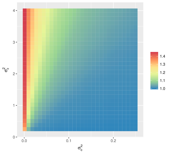
We can, however, inspect how large our concern should be by examining the performance of any of these optimal designs across the possible values of the variance parameters, relative to the performance of the true optimal design at each point. That is, we inspect the ratio of the variance of the intervention effect estimate of a particular design to that of the optimal design at each $(\sigma_{c}^{2},\sigma_{\epsilon}^{2})$ combination. We present such an evaluation in Figure 2 for the following design matrices

$$X_{1}=\begin{pmatrix}0&0&0&0&0&0\\ 0&0&0&0&0&0\\ 0&0&0&0&0&0\\ 0&0&0&0&0&0\\ 0&0&0&0&0&0\\ 1&1&1&1&1&1\\ 1&1&1&1&1&1\\ 1&1&1&1&1&1\\ 1&1&1&1&1&1\\ 1&1&1&1&1&1\\ \end{pmatrix},\qquad X_{2}=\begin{pmatrix}0&0&0&0&0&0\\ 0&0&0&0&0&1\\ 0&0&0&0&0&1\\ 0&0&0&0&1&1\\ 0&0&0&1&1&1\\ 0&0&0&1&1&1\\ 0&0&1&1&1&1\\ 0&1&1&1&1&1\\ 0&1&1&1&1&1\\ 1&1&1&1&1&1\\ \end{pmatrix},$$

which are Designs 8 and 3 from Figure 1 respectively. As must obviously be the case, the value of the ratio of the variances is in all instances at least one. We observe that with the matrix $X_{1}$, the variance of the intervention effect estimate is substantially larger than that for the optimal design when the values of $\sigma_{c}^{2}$ and $\sigma_{\epsilon}^{2}$ are mis-specified, particularly when the value of $\rho$ is in fact large. In contrast, using the matrix $X_{2}$ retains efficient performance in many instances. However, if $\rho$ is small then the variance of the intervention effect provided by this design is still more than 40% larger than that of the optimal design.

Li et al. (2018)[20] recently extended the results of Lawrie et al. (2015)[19] to cohort SW-CRTs. Specifically, they considered a case in which all clusters have to begin in the control condition (intervention 0), and conclude in the experimental (intervention 1). They then demonstrated that the optimal $X$ could be specified by ensuring that the proportion, $p_{t}$, of clusters allocated to a sequence with $t$ ones preceded by $T-t$ zeros satisfies

	$\displaystyle p_{1}$	$\displaystyle=p_{T-1}=\frac{\psi+3\xi}{2\gamma},$
	$\displaystyle p_{t}$	$\displaystyle=\frac{\xi}{\gamma},\qquad\text{ for }t=2,\dots,T-2,$

where

	$\displaystyle\psi$	$\displaystyle=1-(m-1)\rho_{0}-(m-1)\rho_{1}-\rho_{2},$
	$\displaystyle\xi$	$\displaystyle=(m-1)\rho_{1}+\rho_{2},$
	$\displaystyle\gamma$	$\displaystyle=\psi+T\xi.$

Here, we explore their findings for several example design scenarios, again via an exhaustive search. As above, we consider the case in which $\mathfrak{I}=\{6\}$, $\mathfrak{C}=\{\mathfrak{C}_{6}\}=\{10\}$, and $\mathfrak{M}=\mathfrak{M}_{10,6}=\{10\}$, with $\sigma^{2}=1$, $w=0$, and $\beta=1$. To follow their restrictions on the allowed $X$ we enforce that

$$\mathfrak{X}_{6,10}=\{X:\text{dim}(X)=6\times 10,X_{ij}\geq X_{ij-1}\text{ for }j=2,\dots,6\text{ and }i=1\dots,10,X_{i1}=0\text{ and }X_{iT}=1\text{ for }i=1,\dots,C\}.$$

Then, we denote by $\boldsymbol{p}_{\text{th}}=(p_{1},\dots,p_{T-1})^{\top}$ the vector of the $p_{t}$ for the theoretical optimal designs derived by Li et al. (2018),[20] and denote by $\boldsymbol{p}_{\text{emp}}$ the vector of the empirical values of the $p_{t}$ for our identified optimal designs. Our findings are presented in Table 2 for $(\rho_{0},\rho_{1},\rho_{2})\in\{0.05,0.1\}\times\{0.001,0.002\}\times\{0.25,0.5\}$. They illustrate one potential issue with applying the results of Li et al. (2018)[20] in practice; that the theoretically optimal values of the $p_{t}$ will likely not be achievable because $C$ is an integer. However, it is clear that the empirical values of the proportions of clusters changing to the experimental intervention in each time period are close to their theoretical values, even in this case where $C$ is small.

The SO-HIP study is a cross-sectional MA-SW, with $D=3$, to evaluate the effectiveness of sensor monitoring in an occupational therapy rehabilitation program for older people after hip fracture. Specifically, arm 0 corresponds to providing participants with care as usual. Arm 1 then involves the additional use of occupational therapy without sensor monitoring, in contrast to arm 2 that incorporates occupational therapy with cognitive behavioural therapy coaching using sensor monitoring as a coaching tool. Thus, as discussed earlier, intervention $d-1$ is nested within intervention $d$, for $d=1,2$.

SO-HIP plans to enrol six clusters ($C=6$), and have six time periods ($T=6$), with eight observations made per cluster per period ($m=8$), using the following matrix for treatment allocation

$$X=\begin{pmatrix}0&0&0&1&1&2\\ 0&0&0&1&1&2\\ 0&0&1&1&2&2\\ 0&0&1&1&2&2\\ 0&1&1&2&2&2\\ 0&1&1&2&2&2\end{pmatrix}.$$

The trial has $\boldsymbol{\delta}=(1.5\sigma,0.75\sigma)^{\top}$, and assumes that $\sigma_{s}^{2}=\sigma_{\theta}^{2}=0$ and $\rho(=\rho_{0}=\rho_{1}=\rho_{2})=0.05$. With this, when $\sigma^{2}=1$, using our methods described above we can identify that the proposed design will have an individual power of 0.88 ($\beta=0.12$) when the familywise error-rate is controlled to $\alpha=0.05$ using the Bonferroni correction. For further information on this trial, see the published protocol.[25]

We now consider how much efficiency could be gained by utilizing an alternative design. We presume that in the trial any number of time periods two through six could have been employed ($\mathfrak{I}=\{2,\dots,6\}$), and any number of clusters two through six could have actually been utilized ($\mathfrak{C}=\{\mathfrak{C}_{2},\dots,\mathfrak{C}_{6}\}$, with $\mathfrak{C}_{T}=\{2,\dots,6\}$ for each $T\in\mathfrak{T}$). Finally, we assume that the trials plan to recruit 48 patients in total from each cluster would allow $\mathfrak{M}_{C,T}=\{2,\dots,\lfloor 48/T\rfloor\}$. Here, we enforce that

$$\mathfrak{X}_{C,T}=\{X:\text{dim}(X)=C\times T,X_{ij}\geq X_{ij-1}\text{ for }j=2,\dots,T\text{ and }i=1\dots,C\}.$$

Taking our cost function to be the total number of observations, $f(\mathscr{D})=mCT$, we present several admissible designs in Table 3. Explicitly, in this case, we find that the optimal designs when using the D-, A-, and E-optimality criteria coincide for $w=0$ and $w=0.5$. Note that we also considered the optimal designs for $w=1-10^{-4}$, but they were found to be identical to those for $w=0.5$.

We can see that the individual power of the trial could be increased by as much as 12.1%, as a result of reducing the maximum value of the variances of the treatment effect estimators by 44.3% ($w=0$). Alternatively, the individual power could be maintained and the required number of observations reduced by up to 58.3% ($w=0.5$).

References

- [1] A. Atkinson and A. Donev. Optimum Experimental Designs. Oxford University Press, 1992.
- [2] G. Baio, A. Copas, G. Ambler, J. Hargreaves, E. Beard, and R. Omar. Sample size calculation for a stepped wedge trial. Trials, 16:354, 2015.
- [3] T. Benham, Q. Duan, D. Kroese, and B. Liquet. Ceoptim: Cross-entropy r package for optimization. J Stat Soft, 76, 2017.
- [4] M. Chinbuah, P. Kager, M. Abbey, M. Gyapong, E. Awini, J. Nonvignon, M. Adjuik, M. Aikins, F. Pagnoni, and J. Gyapong. Impact of community management of fever (using antimalarials with or without antibiotics) on childhood mortality: a cluster-randomized controlled trial in ghana. Am J Trop Med Hyg, 87:11–20, 2012.
- [5] E. de Hoop, I. van der Tweel, R. van der Graaf, K. Moons, J. van Delden, J. Reitsma, and H. Kofijberg. The need to balance merits and limitations from different disciplines when considering the stepped wedge cluster randomized trial design. BMC Med Res Methodol, 15:93, 2015.
- [6] A. Dmitrienko, C. Chuang-Stein, and R. D’Agostino. Pharmaceutical Statistics Using SAS: A Practical Guide. SAS Institute, 2007.
- [7] A. Donner and N. Klar. Pitfalls of and controversies in cluster randomization trials. Am J Public Health, 94:416–422, 2004.
- [8] S. Edwards, D. Braunholtz, R. Lilford, and A. Stevens. Ethical issues in the design and conduct of cluster randomised controlled trials. BMJ, 318:1407, 1999.
- [9] A. Girling and K. Hemming. Statistical efficiency and optimal design for stepped cluster studies under linear mixed effects models. Stat Med, 35:2149–2166, 2016.
- [10] J. Hargreaves, A. Copas, E. Beard, D. Osrin, J. Lewis, C. Davey, J. Thompson, G. Baio, K. Fielding, and A. Prost. Five questions to consider before conducting a stepped wedge trial. Trials, 16:350, 2015.
- [11] K. Hemming, A. Girling, J. Martin, and S. Bond. Stepped wedge cluster randomized trials are efficient and provide a method of evaluation without which some interventions would not be evaluated. J Clin Epidemiol, 66:1058–1059, 2013.
- [12] K. Hemming, R. Lilford, and A. Girling. Stepped-wedge cluster randomised controlled trials: a generic framework including parallel and multiple level designs. Stat Med, 34:181–196, 2015.
- [13] R. Hooper, S. Teerenstra, E. de Hoop, and S. Eldridge. Sample size calculation for stepped wedge and other longitudinal cluster randomised trials. Stat Med, 35:4718–4728, 2016.
- [14] M. Hussey and J. Hughes. Design and analysis of stepped wedge cluster randomized trials. Contemp Clin Trials, 28:182–191, 2007.
- [15] M. Keriel-Gascou, K. Buchet-Poyau, M. Rabilloud, A. Duclos, and C. C. A stepped wedge cluster randomized trial is preferable for assessing complex health interventions. J Clin Epidemiol, 67:831–833, 2014.
- [16] D. Kotz, M. Spigt, I. Arts, R. Crutzen, and W. Viechtbauer. Researchers should convince policy makers to perform a classic cluster randomized controlled trial instead of a stepped wedge design when an intervention is rolled out. J Clin Epidemiol, 65:1255–1256, 2012a.
- [17] D. Kotz, M. Spigt, I. Arts, R. Crutzen, and W. Viechtbauer. Use of the stepped wedge design cannot be recommended: a critical appraisal and comparison with the classic cluster randomized controlled trial design. J Clin Epidemiol, 65:1249–1252, 2012b.
- [18] D. Kotz, M. Spigt, I. Arts, R. Crutzen, and W. Viechtbauer. The stepped wedge design does not inherently have more power than a cluster randomized controlled trial. J Clin Epidemiol, 66:1059–1060, 2013.
- [19] J. Lawrie, J. Carlin, and A. Forbes. Optimal stepped wedge designs. Stat Probabil Lett, 99:210–214, 2015.
- [20] F. Li, E. Turner, and J. Preisser. Optimal allocation of clusters in cohort stepped wedge designs. Stat Probabil Lett, 137:257–263, 2018.
- [21] V. Lyons, L. Li, J. Hughes, and A. Rowhani-Rahbar. Proposed variations of the stepped-wedge design can be used to accommodate multiple interventions. Stat Med, 86:160–167, 2017.
- [22] J. Matthews and A. Forbes. Stepped wedge designs: insights from a design of experiments perspective. Stat Med, 36:3772–3790, 2017.
- [23] N. Mdege, M.-S. Man, C. Taylor nee Brown, and D. Torgerson. There are some circumstances where the stepped-wedge cluster randomized trial is preferable to the alternative: no randomized trial at all. response to the commentary by kotz and colleagues. J Clin Epidemiol, 65:1253–1254, 2012.
- [24] M. Parmar, J. Carpenter, and M. Sydes. More multiarm randomised trials of superiority are needed. Lancet, 384:283–284, 2014.
- [25] M. Pol, G. Ter Riet, M. van Hartingsveldt, B. Krose, S. de Rooij, and B. Buurman. Effectiveness of sensor monitoring in an occupational therapy rehabilitation program for older persons after hip fracture, the so-hip study: study protocol of a three-arm stepped wedge cluster randomized trial. BMC Health Serv Res, 17:3, 2017.
- [26] A. Prost, A. Binik, I. Abubakar, A. Roy, M. De Allegri, C. Mouchoux, T. Dreischulte, H. Ayles, J. Lewis, and D. Osrin. Logistic, ethical, and political dimensions of stepped wedge trials: critical review and case studies. Trials, 16:351, 2015.
- [27] S. Teerenstra and H. Calsbeek. Stepped-wedge like designs to compare active implementation strategies with natural development in absence of active implementation. Presented at the 36th Annual Conference of the International Society for Clinical Biostatistics, Utrecht, The Netherlands, August 23-27, 2015.
- [28] J. Thompson, K. Fielding, J. Hargreaves, and A. Copas. The optimal design of stepped wedge trials with equal allocation to sequences and a comparison to other trial designs. Clin Trials, 14:639–647, 2017.
- [29] A. Vickers. Clinical trials in crisis: four simple methodologic fixes. Clin Trials, 11:615–621, 2014.
- [30] J. Wason, L. Stecher, and A. Mander. Correcting for multiple-testing in multi-arm trials: is it necessary and is it done? Trials, 15:364, 2014.
- [31] W. Woertman, E. de Hoop, M. Moerbeek, S. Zuidema, D. Gerritsen, and S. Teerenstra. Stepped wedge designs could reduce the required sample size in cluster randomized trials. J Clin Epidemiol, 66:752–758, 2013.