Convergence analysis of a finite element approximation of minimum action methods
Abstract
In this work, we address the convergence of a finite element approximation of the minimizer of the Freidlin-Wentzell (F-W) action functional for non-gradient dynamical systems perturbed by small noise. The F-W theory of large deviations is a rigorous mathematical tool to study small-noise-induced transitions in a dynamical system. The central task in the application of F-W theory of large deviations is to seek the minimizer and minimum of the F-W action functional. We discretize the F-W action functional using linear finite elements, and establish the convergence of the approximation through -convergence.
keywords
large deviation principle, minimum action method, convergence analysis, non-gradient system, phase transitionAMS
65M60, 65P40, 65K101 Introduction
We consider a general dynamical system perturbed by small noise
| (1) |
where is a small positive number and is a standard Wiener process in . The long-term behavior of the perturbed system is characterized by the small-noise-induced transitions between the equilibriums of the unperturbed system
| (2) |
These transitions rarely occur but have a major impact. This model can describe many critical phenomena in physical, chemical, and biological systems, such as non-equilibrium interface growth [10, 18], regime change in climate [29], switching in biophysical network [28], hydrodynamic instability [26, 27], etc.
The Freidlin-Wentzell (F-W) theory of large deviations provides a rigorous mathematical framework to understand the small-noise-induced transitions in general dynamical systems, where the key object is the F-W action functional, and the critical quantities include the minimizer and minimum of the F-W action functional [11]. Starting from [6], the large deviation principle given by the F-W theory has been approximated numerically, especially for non-gradient systems, and the numerical methods are, in general, called minimum action method (MAM). More specifically, the following optimization problems need to be addressed:
| (3) |
and
| (4) |
where
| (5) |
is called the action functional. Here is a path connecting and in the phase space on the time interval . The minima and minimizers of Problems I and II characterize the difficulty of the small-noise-induced transition from to the vicinity of , see equations (6) and (8). In Problem I, the transition is restricted to a certain time scale , which is relaxed in Problem II. Let be the minimizer of either Problem I or Problem II, which is also called the minimal action path (MAP), or the instanton in physical literature related to path integral. For problem II, we have an optimal integration time which can be either finite or infinite depending on the states and .
We will focus on the minimum action method for non-gradient systems. For gradient systems, the minimal action path is consistent with the minimum energy path, and the counterpart version of minimum action method includes string method [6], nudged elastic band method [15], etc., which takes advantage of the property that the minimal action path is parallel to the drift term of the stochastic differential equation. For non-gradient systems, this property does not hold and a direct optimization of the F-W action functional needs to be considered. The main numerical difficulty comes from the separation of slow dynamics around critical points from fast dynamics elsewhere. More specifically, the MAP will be mainly captured by the fast dynamics subject to a finite time, but it will take infinite time to pass a critical point. To overcome this difficulty, there exist two basic techniques: (1) non-uniform temporal discretization, and (2) reformulation of the action functional with respect to arc length. Two typical techniques to achieve non-uniform temporal discretization include moving mesh technique and adaptive finite element method. The moving mesh technique starts from a uniform finite mesh and redistributes the grid points iteratively such that more grids are assigned into the region of fast dynamics and less grids into the region of slow dynamics. This technique is used by the adaptive minimum action method (aMAM) [30, 21, 23, 19]. The adaptive finite element method starts from a coarse mesh and has an inclination to refine the mesh located in the region of fast dynamics [24, 25]. The main difference of these two techniques from the efficiency point of view is that the moving mesh technique needs a projection from fine mesh to fine mesh, i.e., global reparameterization, while the adaptive finite element method only needs local projection in the elements that have been refined. To eliminate the scale separation from dynamics, one can consider parameterization of the curves geometrically, i.e., a change of variable from time to arc length, which is used in the geometric minimum action method (gMAM) [14, 12, 13]. The change of variable induces two difficulties. One is related to accuracy and the other one is related to efficiency. The mapping from time to arc length is nonlinear and the Jacobian of the transform between time and arc length variables is singular around critical points since an infinite time domain has been mapped to a finite arc length. Unknown critical points along the minimal action path may deteriorate the approximation accuracy unless they can be identified accurately. To use arc length for parameterization, we have that the velocity is a constant, which means in each iteration step a global reparameterization is needed to maintain this constraint.
Both aMAM and gMAM target to the case that . In aMAM, a finite but large is used while in gMAM, the infinite is mapped to a finite arc length. So, aMAM is not able to deal with Problem II subject to a finite since a fixed is required while gMAM is not able to deal with Problem I since has been removed. To deal with both Problem I and II in a more consistent way, we have developed a minimum action method with optimal linear time scaling (temporal minimum action method, or tMAM) coupled with adaptive finite element discretization [24, 25]. The method is based on two observations: (1) for any given transition path, there exists a unique to minimize the action functional subject to a linear scaling of time, and (2) for transition paths defined on a finite element approximation space, the optimal integration time is always finite but increases as the approximation space is refined. The first observation removes the parameter in Problem II and the second observation guarantees that the discrete problem of Problem II is well-posed after is removed. Problem I becomes a special case of our reformation of Problem II. This way, tMAM is able to deal with both Problem I and II.
Although many techniques have been developed from the algorithm point of view, few numerical analysis has been done for minimum action method. We want to fill this gap partially in this work. We consider a general stochastic ordinary differential equation (ODE) system (1). The discrete action functional will be given by linear finite elements for simplicity, where indicates the element size. Due to the general assumption for , we will focus on the convergence of the minimizers of as and only provide a priori error estimate for the approximate solution when is a linear symmetric positive definite (SPD) system. For Problem I, the convergence of the minimizer to is established by the -convergence of the discretized action functional. For Problem II, we employ and analyze the strategy developed in [24] to deal with the optimization with respect to . More specifically, we reformulate the problem from to by a linear time scaling and replace the integration time with a functional with , where is the optimal integration time for a given transition path . When is finite, the convergence of the minimizer to can be established by the -convergence of the discretized action functional. When , the linear mapping from to does not hold. We demonstrate that the sequence still provides a minimizing sequence as and establish the convergence using the results from gMAM. Due to the nonlinearity of , the Euler-Lagrange (E-L) equation associated with the action functional is, in general, a nonlinear elliptic problem for Problem I. For problem II subject to a optimal linear time scaling, the E-L equation remains the same form as Problem I with the parameter being replaced by a functional , which becomes a nonlocal and nonlinear elliptic equation. When is a linear SPD system, we are able to establish the a priori error estimate for , where the E-L equation is a nonlocal and nonlinear elliptic problem of Kirchhoff type.
The remain part of this paper is organized as follows. In Section 2, we describe the problem setting. A reformulation of the Freidlin-Wentzell action functional is given in Section 3 to deal with the optimization with respect to in Problem II. We establish the convergence of finite element approximation in Section 4 for general stochastic ODE systems. In Section 5, we apply our method to a linear stochastic ODE system and provide a prior error estimate of the approximation solution. Numerical illustrations are given in Section 6 followed by a summary section.
2 Problem description
We consider the small-noise-perturbed dynamical system (1). Let and be two arbitrary points in the phase space. The Freidlin-Wentzell theory of large deviations provides asymptotic results to estimate the transition probability from to the vicinity of when . If we restrict the transition on a certain time interval , we have
| (6) |
where is the first entrance time of the -neighborhood of for the random process starting from . The path variable connecting and , over which the action functional is minimized, is called a transition path. If the time scale is not specified, the transition probability can be described with respect to the quasi-potential from to :
| (7) |
The probability meaning of is
| (8) |
We in general call the asymptotic results given in equations (6) and (8) large deviation principle (LDP). We use to indicate transition path that minimizes the action functional in equation (6) or (8), which is also called the minimal action path (MAP) [7]. The MAP is the most probable transition path from to . For the quasi-potential, we let indicate the optimal integration time, which can be either finite or infinite depending on and . The importance of LDP is that it simplifies the computation of transition probability, which is a path integral in a function space, to seeking the minimizers or . From the application point of view, one central task of Freidlin-Wentzell theory of large deviations is then to solve the Problem I and Problem II defined in (3) and (4), correspondingly. For Problem II, we need to optimize the action functional with respect to the integration time . We will present a reformulation of in Section 3 to deal with this case.
To analyze the convergence properties of numerical approximations for Problem I and II, we need some assumptions on .
Assumption 1.
- (1)
is Lipschitz continuous in a big ball, i.e., there exist constants and , such that
(9) where denotes the norm of a vector in ;
- (2)
There exist positive numbers , such that
(10) where , and
- (3)
The solution points of are isolated.
Lemma 2.
Let assumption (10) hold. If both the starting and ending points of a MAP are inside , then is located within for any .
Proof.
Suppose that is a MAP outside of but connecting two points and on the the surface of . Let . We have
| (11) |
Taking inner product on both sides of the above equation with , we get
| (12) |
Then by using Cauchy’s inequality with , and assumption (10), we get
| (13) |
Taking integration, and using the definition of minimum action, we obtain a bound for any along the MAP:
| (14) |
which means that the whole MAP is located within . ∎
Remark 2.1.
The assumptions (9) and (10) allow most of the physically relevant smooth nonlinear dynamics. It is seen from Lemma 2 that the second assumption (10) is used to restrict all MAPs of interest inside . For simplicity and without loss of generality, we will assume from now on that the Lipschitz continuity of is global, namely, . For the general case given in Assumption 1, one can achieve all the conclusions by restricting the theorems and their proofs into .
We now summarize some notations that will be used later on. For defined on , we let and , where is the -th component of and . We let , where . For defined on , we define the inner products and .
3 A reformulation of
We start with a necessary condition given by Maupertuis’ principle of least action for the minimizer of Problem II.
Lemma 3 ([14]).
Let be the minimizer of Problem II. Then is located on the surface , where is the Hamiltonian given by the Legendre transform of . More specifically, for equation (1)
| (15) |
We will call equation (15) the zero-Hamiltonian constraint in this paper. The zero-Hamiltonian constraint defines a nonlinear mapping between the arc length of the geometrically fixed lines on surface and time (see Section 4.3.1 for more details). We instead consider a linear time scaling on , which is simpler and more flexible for numerical approximation. For any given transition path and a fixed , we consider the change of variable . Let Then and we rewrite the action functional as
| (16) |
Lemma 4.
For any given transition path , we have
| (17) |
if , where
| (18) |
Proof.
It is easy to verify that the functional is nothing but the unique solution of the optimality condition . ∎
Corollary 5.
Let be the minimizer of Problem II. If , we have , where .
Proof.
From the zero-Hamiltonian constraint (15) and the definition of , we have
Integrating both sides on , we have the conclusion. ∎
For any absolutely continuous path , it is shown in Theorem 5.6.3 in [5] that can be written as
| (19) |
This means that we can seek the MAP in the Sobolev space . From now on, we will use to indicate if no ambiguity arises. The same rule will be applied to other spaces such as and .
We define the following two admissible sets consisting of transition paths:
| (20) | ||||
| (21) |
where we let and just for convenience.
Lemma 6.
Proof.
Conversely, if is a minimizer of , we let and for We have
when . Then is a minimizer of . So the minimizers of and have a one-to-one correspondence when the optimal integral time is finite. ∎
4 Finite element discretization of Problems I and II
The numerical method to approximate Problems I and II is usually called minimum action method (MAM) [7]. Many versions of MAM have been developed, where the action functional is discretized by either finite difference method or finite element method. In this work, we consider the finite element discretization of and focus on the convergence of the finite element approximation of the minimizer.
Let and be partitions of and , respectively. We define the following approximation spaces given by linear finite elements:
For any we define the following discretized action functionals:
| (24) |
and
| (25) |
We note that for a fixed integration time , we can rewrite as by letting , such that Problem I can also be defined on . Since we intend to use the reformulation to deal with the parameter in Problem II, we use and to define Problem I and II, respectively, for clarity.
4.1 Problem I with a fixed
For this case, our main results are summarized in the following theorem:
Theorem 7.
For Problem I with a fixed , we have
namely, the minima of converge to the minimum of as Moreover, if is a sequence of minimizers of then there is a subsequence that converges weakly in to some which is a minimizer of
The proof of this theorem will be split into two steps: (1) the existence of the minimizer of in , and (2) -convergence of to as .
4.1.1 Solution existence in
We search the minimizer of in the admissible set . The solution existence is given by the following lemma.
Lemma 8.
There exists at least one function such that
Proof.
We first establish the coerciveness of In order to do so, we define an auxiliary function by
Then and Since is globally Lipschitz continuous, we have
By Gronwall’s inequality, we have
from which we obtain
where and are two positive constants depending on and . Thus, the action functional satisfies
The coerciveness follows. On the other hand, the integrand is bounded below by and convex in By the Theorem 2 on Page 448 in [9], is weakly lower semicontinuous on
For any minimizing sequence from the coerciveness, we have
Let be any fixed function, e.g., the linear function on from to Then and
by the Poincaré’s Inequality. Thus is bounded in Then there exists a subsequence converging weakly to some in Then converges to weakly in By Mazur’s Theorem [9], is weakly closed. So , i.e.,
Therefore, Since we reach the conclusion. ∎
4.1.2 -convergence of
We first note the following simple property:
Property 9.
For any sequence converging weakly to , we have
Proof.
Since converges weakly to in , in , i.e., converges strongly to in the sense. By the Lipschitz continuity of , we reach the conclusion. ∎
We now establish the -convergence of :
Lemma 10 (-convergence of ).
Let be a sequence of finite element meshes with . For every , the following two properties hold:
- •
Lim-inf inequality: for every sequence converging weakly to in we have
(26) - •
Lim-sup inequality: there exists a sequence converging weakly to in such that
(27)
Proof.
We first address the lim-inf inequality. We only need to consider a sequence since otherwise, (26) is trivial by the definition of Let be an arbitrary sequence converging weakly to in . The action functional can be written as
| (28) |
The functional defined by is obviously weakly lower semicontinuous in since the integrand is convex with respect to .
For in equation (28). We have
Using Property 9 and the fact that , we have that the first term of the above inequality converges to . Moreover, the second term also converges to due to the weak convergence of to in . Thus,
Combining the results for , and , we obtain
which yields the lim-inf inequality.
We now address the lim-sup inequality. Since is dense in , for any and , there exists a non-zero such that We have
by letting
where is an interpolation operator defined by linear finite elements. Let Then we have and
and
as So converges to in and also converges weakly in . By Property 9, we know that in . Thus,
which yields the lim-sup equality. ∎
4.1.3 Proof of Theorem 7
With the solution existence and the -convergence being proved, we only need the equi-coerciveness of for the final conclusion. For any , we have Then the equi-coerciveness of in follows from the coerciveness of restricted to (see the first step in the proof of Lemma 8).
4.2 Problem II with a finite
For this case, we consider the reformulation of given in Section 3. From Lemma 6, we know that Problem II with a finite is equivalent to minimizing in (see equation (22)). Our main results are summarized in the following theorem:
Theorem 11.
For Problem II with a finite , we have
namely, the minima of converge to the minimum of as Moreover, if is a sequence of minimizers of then there is a subsequence that converges weakly in to some which is a minimizer of
Similar to Problem I with a fixed , we split the proof of this theorem into two steps: (1) the existence of the minimizer of in , and (2) -convergence of to as .
4.2.1 Solution existence in
We start from the following property of the functional .
Property 12.
There exists a constant such that
| (29) |
for any .
Proof.
For any let , where and is a linear function connecting and . We have
where is the constant for Poincaré’s Inequality. So
where and
Let be a perturbation function with . We have
where is the remainder term of .
We then have the first-order variation of as
The optimality condition yields two possible cases: and For the first case, is a constant. But so Then For the second case, Thus,
More specifically,
∎
We search the minimizer of in the admissible set . The solution existence is given by the following lemma.
Lemma 13.
If the optimal integral time for Problem II is finite, there exists at least one function such that
Proof.
We first establish the weakly lower semi-continuity of in . Rewrite by substituting (18) to get
For any sequence converging weakly to in , is bounded in and in . Coupling with the global Lipschitz continuity of , we can obtain
The weakly lower semicontinuity of yields that
| (30) |
Combining the above results, we obtain
that is, is weakly lower semicontinuous in
We subsequently establish the coercivity of . Since is finite, there exists such that
In fact, by Lemma 6, a minimizing sequence of defines a minimizing sequence of which also corresponds to a minimizing sequence of . The assumption of allows us to add the condition that . Otherwise, must go to infinity. The continuity of with respect to yields that , which contradicts our assumption that . Now, let Then for any with
By Gronwall’s Inequality, we have
which yields that
| (31) |
where only depend on and So
where we used Property 12 in the last step. This is the coercivity.
For any minimizing sequence of , we have
Let . Then
by Poincaré’s Inequality. Thus, is bounded in Then there is a subsequence converging to some weakly in So converges weakly to in By Mazur’s Theorem, is weakly closed. So and By Lemma 6, corresponding to is a minimizer of and . ∎
4.2.2 -convergence of
The -convergence of with respect to parameter is established in the following lemma:
Lemma 14 (-convergence of ).
Let be a sequence of finite element meshes. For every , the following two properties hold:
- •
Lim-inf inequality: for every sequence converging weakly to in we have
(32) - •
Lim-sup inequality: there exists a sequence converging weakly to in such that
(33)
Proof.
We first address the lim-inf inequality. We only consider sequence otherwise, the inequality is trivial. Similar to the proof of Lemma 13, rewrite the discretized functional as
By the same argument as in the proof of Lemma 10, we have
Combining these results, we have the lim-inf inequality. The lim-sup inequality can be obtained by the same argument as in the proof of Lemma 10 ∎
4.2.3 Proof of Theorem 11
4.3 Problem II with an infinite
When is infinite, the integration domain becomes the whole real space, corresponding to a degenerate case of linear scaling. To remove the optimization parameter , the zero-Hamiltonian constraint (15) can be considered under another assumption that the total arc length of is finite, which is the basic idea of the geometric MAM (gMAM) [14]. However, since the Jacobian of the transform between time and arc length variables will become singular at critical points, the numerical accuracy will deteriorate when unknown critical points exist along the MAP.
We will still work with the formulation with respect to time, which means that we need to use a large but finite integration time to deal with the case . We discuss this case by considering a relatively simple scenario, but the numerical difficulties are reserved. Let be an asymptotically stable equilibrium point, is contained in the basin of attraction of , and for any , where is the exterior normal to the boundary . Then starting from any point in , a trajectory of system (2) will converge to . We assume that the ending point of Problem II is located on .
4.3.1 Escape from the equilibrium point
If we consider the change of variable in general, say , we have (see Lemma 3.1, Chapter 4 in [11])
| (34) |
where , is the derivative with respect to , and the equality holds if the zero-Hamiltonian constraint (15) is satisfied. With respect to , the zero-Hamiltonian constraint can be written as
| (35) |
from which we have
| (36) |
If , the variable is nothing but a rescaled arc length. Assuming that the length of the optimal curve is finite, we can rescale the total arc length to one, i.e., , which yields the geometric minimum action method (gMAM) [14].
We now look at any transition path that satisfies the zero-Hamiltonian constraint. Let corresponds to the arc length with , then . Let be an arbitrary point on . Then the integration time from to is
where is the arc length of the curve connecting and , i.e., the value of the arc length variable at point . Note that if the end point is in a small neighborhood of the equilibrium , the total arc length from to along is small. However, from the fact
we get
as long as . So , because is a critical point.
For clarity, we include the starting and ending points of the transition path into some notations. Let indicate the minimizer of Problem II with starting point and ending point , and let be the corresponding optimal integration time. We have for any on , and for the exit problem as long as the has a finite length.
4.3.2 Minimizing sequence for
Let be the linear function connecting 0 and in one time unit . Then
where . Although for any finite , the action decreases with respect to to zero. We consider a sequence of optimization problems
| (37) |
generated by the constraint . We have that
Lemma 15.
is a minimizing sequence of (23).
Proof.
First of all, is decreasing as increases. Pick one such that and consider a sequence of , . Let be the first intersection point of and when traveling along from to , so . The optimal transition time . We construct a path from to as follows:
Due to the additivity, we know that is located on since . Then is a minimizing sequence as decreases, and
Consider . We have
where the first inequality is because is, in general, not equal to . We then reach the conclusion. ∎
When , we have as goes close to the minimizer, implying that . Thus for this case, we cannot study the convergence in . A larger space is needed, i.e., the space consisting of absolutely continuous functions. So we use , the space of absolutely continuous functions connecting and on with . To prove the convergence of the minimizing sequence in Lemma 15, we use the following lemma, which is Proposition 2.1 proved in [14]:
Lemma 16.
Assume that the sequence with and for every , is a minimizing sequence of (7) and that the lengths of the curves of are uniformly bounded, i.e.
Then the the action functional has a minimizer , and for some subsequence we have that
where denotes the Fréchet distance.
Theorem 17.
Assume that the lengths of the curves are uniformly bounded. Then there exists a subsequence that converges to a minimizer with respect to Fréchet distance.
Proof.
Although we just constructed for an exit problem around the neighborhood of an asymptotically stable equilibrium, it is easy to see that the idea can be applied to a global transition, say both and are asymptotically stable equilibrium, as long as there exist finitely many critical points along the minimal action path. In equation (37), we introduced an extra constraint , which implies that the infimum may be reached at the boundary . From the optimization point of view, such a box-type constraint is not favorable. Next, we will show that this constraint is not needed for the discrete problem.
4.3.3 Remove the constraint for a discrete problem
The key observation is as follows:
Lemma 18.
If is the minimizer of over , then , for any given .
Proof.
We argue by contradiction. Note that
where the last inequality is from the inverse inequality of finite element discretization and the constant only depends on mesh [3]. If , we have two possible cases: or . The first case implies that for all , which contradicts (3) of Assumption 1. The second case implies that must go to infinity somewhere due to the continuity, which contradicts Lemma 2. ∎
Lemma 18 means that for a discrete problem the constraint in equation (37) is not necessary in the sense that there always exists a number such that . We can then consider a sequence of finite element meshes and treat the minimization of exactly in the same way as the case that is finite. Simply speaking, defines a minimizing sequence as no matter that is finite or infinite. The only difference between and is that we address the convergence of in for and in for .
4.3.4 The efficiency of
The E-L equation associated with is:
| (38) |
For a fixed , the E-L equation associated with is the same as equation (38) except that we need to replace with [24]. If , as , which means that the E-L equation (38) eventually becomes degenerate. When is small, is finite but large. Equation (38) can be regarded as a singularly perturbed problem, which implies the possible existence of boundary/internal layers. Thus the minimizing sequence given by a uniform refinement of may not be effective.
Consider a transition from a stable fixed point to a saddle point without any other critical points on the minimal transition path. The dynamics is slow around the critical points and fast else where, which means that for the approximation given by a fixed large , the path will be mainly captured in a subinterval with with respect to the scaled time . Then an effective has a fine mesh for and a coarse mesh for . Currently, there exist two techniques to achieve an effective nonuniform discretization : (1) Moving mesh technique. Starting from a fine uniform discretization, the grid points will be redistributed such that more grid points will be moved from the region of slow dynamics to the region of fast dynamics [30, 21]. This procedure needs to be iterated until the optimal nonuniform mesh is reached with respect to a certain criterion for the redistribution of grids. (2) Adaptive finite element method. Starting from a coarse uniform mesh, will be refined adaptively such that more elements will be put into the region of fast dynamics and less elements into the region of slow dynamics [24, 25]. Numerical experiments have shown that both techniques can recover the optimal convergence rate with respect to the number of degrees of freedom.
5 A priori error estimate for a linear ODE system
In this section we apply our strategy to a linear ODE system with , where is a symmetric positive definite matrix. Then is a global attractor. The E-L equation associated with becomes
| (39) |
which is a nonlocal elliptic problem of Kirchhoff type. For Problem I with a fixed , i.e., , equation (39) becomes a standard diffusion-reaction equation.
Let be the minimizer of , and the minimizer of , where is a linear function connecting and on . Let
For a fixed , equation (39) has a unique solution and the standard argument shows that
| (40) |
If is large enough, equation (39) can be regarded as a singularly perturbed problem, the best approximation given by a uniform mesh cannot reach the optimal convergence rate due to the existence of boundary layer.
We now consider Problem II with a finite . The minimizer of satisfies the weak form of equation (39):
| (41) |
The minimizer of satisfies the discrete weak form:
| (42) |
We have the following a priori error estimate for Problem II with a finite :
Proposition 19.
Proof.
Let be the best approximation of on , i.e.,
We then have
where . Consider
| (44) |
We look at first. Note that
| (45) |
where
and is the Poincaré constant. Then we have
| (46) |
By the definition of , we have
We then have
where .
To this end, we obtain a similar a priori error estimate to that for Problem I with a fixed . Since can be arbitrarily large, we know that the optimal convergence rate may degenerate when a boundary layer exists. Using Proposition 19, we can easily obtain the optimal convergence rate with respect to the error of action functional:
| (47) |
where the second-order variation can be obtained with respect to the perturbation function .
The convergence rate for is also optimal. For a general case, we have the first-order variation of at with a test function as
Also note that the second order variation has the same order as . Let . From Proposition 19, we know the second-order variation has an optimal convergence rate , when . If can also reach its optimal rate, which is of order , the overall convergence rate for is of order . We will not analyze the optimal convergence of in norm here, but only provide numerical evidence of the optimal convergence rate for in the next section.
6 Numerical experiments
We will use the following simple linear stochastic ODE system to demonstrate our analysis results
| (48) |
where
with , , , and . Then is a stable fixed point. For the corresponding deterministic system, namely when , and any given point in the phase space, the trajectory converges to as . When noise exists, this trajectory is also the minimal action path from to with , since . Moreover, if the ending point is , . This obviously is not an exit problem, which is a typical application of MAM. However, it includes most of the numerical difficulties of MAM, and the trajectory can serve as an exact solution, which simplifies the discussions.
Consider the minimal action path from () to such that . Since the minimal action path corresponds to a trajectory, we can use the value of action functional as the measure of error with an optimal rate (see equation (47)), where is the number of elements. We will look at the following two cases:
- 1.
- 2.
. We will compare the convergence behavior between tMAM and MAM with a fixed large . According to Theorem 17, we have the convergence in . However, the convergence behavior of this case is similar to that for a finite but large , where we expect a deteriorated convergence rate.
6.1 Case (i)
Let . We use as the ending point such that . In figure 1 we plot the convergence behavior of tMAM with uniform linear finite element discretization. It is seen that the optimal convergence rate is reached for both action functional and estimated by .


6.2 Case (ii)
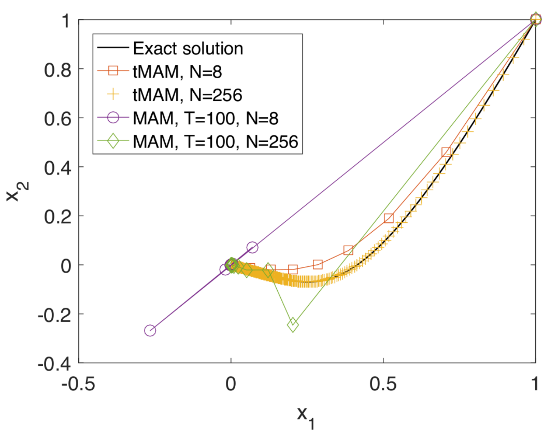
For this case, we still use as the starting point. The ending point is chosen as such that . Except tMAM, we use MAM with a fixed to approximate this case, where is supposed to be large. In general, we do not have a criterion to define how large is enough because the accuracy is affected by two competing issues: 1) The fact that favors a large ; but 2) a fixed discretization favors a small . This implies that for any given , an “optimal” finite exists. For the purpose of demonstration, we choose , which is actually too large from the accuracy point of view. Let be the approximate MAP given by MAM with a fixed . We know that yields a smaller action with the integration time . In this sense, no matter what is chosen, for the same discretization tMAM will always provide a better approximation than MAM with a fixed . The reason we use an overlarge is to demonstrate the deterioration of convergence rate. In figure 2, we plot the convergence behavior of tMAM and MAM with on the left, and the estimated given by tMAM on the right. It is seen that the convergence is slower than as we have analyzed in section 5. For the same discretization, tMAM has an accuracy that is several orders of magnitude better than MAM with . In the right plot of figure 2, we see that the optimal integration time for a certain discretization is actually not large at all. This implies that MAM with a fixed for Case (ii) is actually not very reliable. In figure 3, we compare the MAPs given by tMAM and MAM with the exact solution , where all symbols indicate the nodes of finite element discretization. First of all, we note that the number of effective nodes in MAM is small because of the scale separation of fast dynamics and small dynamics. Most nodes are clustered around the fixed point. This is called a problem of clustering (see [19, 25] for the discussion of this issue). Second, if the chosen is too large, oscillation is observed in the paths given by MAM especially when the resolution is relatively low; on the other hand, tMAM does not suffer such an oscillation by adjusting the integration time according to the resolution. Third, although tMAM is able to provide a good approximation even with a coarse discretization, more than enough nodes are put into the region around the fixed point, which corresponds to the deterioration of convergence rate. To recover the optimal convergence rate, we need to resort to adaptivity (see [24, 25] for the construction of the algorithm).
7 Summary
In this work, we have established some convergence results of minimum action methods based on linear finite element discretization. In particular, we have demonstrated that the minimum action method with optimal linear time scaling, i.e., tMAM, converges for Problem II no matter that the optimal integration time is finite or infinite.
Acknowledgement
X. Wan and J. Zhai were supported by AFOSR grant FA9550-15-1-0051 and NSF Grant DMS-1620026. H. Yu was supported by NNSFC Grant 11771439,91530322 and Science Challenge Project No. TZ2018001.
References
- [1] A. Braides, -Convergence for Beginners, Oxford University Press, 2002.
- [2] A. Braides, Local Minimization, Variational Evolution and -Convergence, Lecture Notes in Mathematics, vol 2094, Springer, Berlin, 2014.
- [3] P. G. Ciarlet, The Finite Element Method for Elliptic Problems, SIAM, 2002.
- [4] G. Dal Maso, An Introduction to -convergence, Birkhauser, Boston, 1993.
- [5] A. Dembo and O. Zeitouni, Large Deviations Techniques and Applications, 2nd ed., Springer, 1998.
- [6] W. E, W. Ren and E. Vanden-Eijnden, String method for the study of rare events, Phys. Rev. B, 66 (2002), 052301.
- [7] W. E, W. Ren and E. Vanden-Eijnden, Minimum action method for the study of rare events, Commun. Pure Appl. Math., 57 (2004), 637–656.
- [8] W. E, W. Ren and E. Vanden-Eijnden, Simplified and improved string method for computing the minimum energy paths in barrier-crossing events, J. Chem. Phys., 126 (2007), 164103.
- [9] L. C. Evans, Partial Differential Equations, American Mathematical Society, 2nd Edition, 2010.
- [10] H.C. Fogedby and W. Ren, Minimum action method for the Kardar-Parisi-Zhang equation, Phys. Rev. E, 80 (2009), 041116.
- [11] M. Freidlin and A. Wentzell, Random Perturbations of Dynamical Systems, second ed., Springer-Verlag, New York, 1998.
- [12] T. Grafke, R. Grauer, T. Schäfer and E. Vanden-Eijnden, Arclength parametrized Hamilton’s equations for the calculation of instantons, SIAM, Multiscale Model. Simul., 12(2) (2014), 566–580.
- [13] T. Grafke, T. Schäfer and E. Vanden-Eijnden, Long-term effects of small random perturbations on dynamical systems: theoretical and computational tools, In: R. Melnik, R. Makarov and J. Belair (eds), Recent Progress and Modern Challenges in Applied Mathematics, Modeling and Computational Science, Fields Institute Communications, vol 79. Springer, New York, NY.
- [14] M. Heymann and E. Vanden-Eijnden, The geometric minimum action method: A least action principle on the space of curves, Commun. Pure Appl. Math., 61 (2008), 1052-1117.
- [15] H. Jònsson, G. Mills and K. Jacobsen, Nudged elastic band method for finding minimum energy paths of transitions, Classical and Quantum Dynamics in Condensed Phase Simulations, Ed. B. Berne, G. Ciccotti and D. Coker, 1998.
- [16] S. Kesavan, Topics in Functional Analysis and Applications, John Wiley & Sons Inc., 1989.
- [17] J. Nocedal and S. Wright, Numerical Optimization, Springer Series in Operations Research, Springer, New York, 1999.
- [18] N. R. Smith, B. Meerson and P. V. Sasorov, Local average height distribution of fluctuating interfaces, Phys. Rev. E, 95 (2017), 012134.
- [19] Y. Sun and X. Zhou, An improved adaptive minimum action method for the calculation of transition path in non-gradient systems, Comm. Comput. Phys., 24(1) (2018), 44–68.
- [20] X. Wan, X. Zhou and W. E, Study of the noise-induced transition and the exploration of the configuration space for the Kuramoto-Sivashinsky equation using the minimum action method, Nonlinearity, 23 (2010), 475-493.
- [21] X. Wan, An adaptive high-order minimum action method, J. Comput. Phys., 230 (2011), 8669-8682.
- [22] X. Wan, A minimum action method for small random perturbations of two-dimensional parallel shear flows, J. Comput. Phys., 235 (2013), 497–514.
- [23] X. Wan and G. Lin, Hybrid parallel computing of minimum action method, Parallel Computing, 39 (2013), 638–651.
- [24] X. Wan, A minimum action method with optimal linear time scaling, Comm. Comput. Phys., 18(5) (2015), 1352–1379.
- [25] X. Wan, B. Zheng and G. Lin, An -adaptive of minimum action method based on a posteriori error estimate, Comm. Comput. Phys., 23(2) (2018), 408–439.
- [26] X. Wan, H. Yu and W. E, Model the nonlinear instability of wall-bouned shear flows as a rare event: A study on two-dimensional Poiseuille flows, Nonlinearity, 28 (2015), 1409–1440.
- [27] X. Wan and H. Yu, A dynamic-solver-consistent minimum action method: With an application to 2D Navier-Stokes equations, J. Comput. Phys., 33 (2017), 209–226.
- [28] D. K. Wells, W. L. Kath and A. E. Motter, Control of stochastic and induced switching in biophysical networks, Phys. Rev. X 5 (2015), 031036.
- [29] W. Yao and W. Ren, Noise-induced transition in barotropic flow over topography and application to Kuroshio, J. Comput. Phys. 300 (2015), 352-364.
- [30] X. Zhou, W. Ren and W. E, Adaptive minimum action method for the study of rare events, J. Chem. Phys., 128 (2008), 104111.
- [31] X. Zhou and W. E, Study of noise-induced transitions in the Lorenz system using the minimum action method, Comm. Math. Sci., 8(2) (2010), 341-355.