Criticality at absolute zero from Ising model on two-dimensional dynamical triangulations
Abstract
We reconsider the criticality of the Ising model on two-dimensional dynamical triangulations based on the Hermitian two-matrix model with the introduction of a loop-counting parameter and linear terms in the potential. We show that in the large- limit even though the Ising model is classical, the critical temperature can reach absolute zero by tuning the loop-counting parameter, and the corresponding continuum theory turns out to be the quantised theory of neither pure gravity nor gravity coupled to conformal matter with central charge being .
1 Introduction
Two-dimensional dynamical triangulations (d DT), first introduced in [1, 2, 3, 4, 5, 6], are a quite powerful method to regularise two-dimensional Euclidean quantum gravity (Liouville quantum gravity) coupled to conformal matter with central charge less than or equal to one, or equivalently worldsheets of non-critical string theories embedded in dimensions less than or equal to one (see e.g. [7, 8]). With the help of matrix-model descriptions, statistical systems on d DT have been studied quite well, and the Ising model on d DT, which can be described by the Hermitian two-matrix model [9, 10], is an example. In the large- limit, this model can be solved exactly when external magnetic field is zero and the critical exponents of the Ising model dressed by quantum gravity turn out to be different [10] from Onsager’s exponents on a two-dimensional flat regular lattice, known as the Knizhnik-Polyakov-Zamolodchikov (KPZ) exponents [11], which originates with the existence of two kinds of divergent fluctuations associated with triangulations as well as Ising spins at the critical point. The field theory obtained by the continuum limit around the critical point is known to be the quantised theory of two-dimensional Euclidean gravity coupled to conformal matter with central charge being [9].
Two-dimensional causal dynamical triangulations (d CDT) [12], whose ensembles are different from those of d DT 11 1 CDT is defined with the Lorentzian signature, but one can move to the Euclidean signature by an analytic continuation, which directly maps individual triangulations (e.g. see [13]). In this paper we consider CDT with the Euclidean signature. , i.e. no baby-universe creation is allowed, are known to provide a regularisation for the two-dimensional projectable Hořava-Lifshitz quantum gravity [14]. CDT is closer to regular triangulations than DT in the sense that back-reactions of triangulations on matter are small compared to those of DT, e.g. critical exponents of the Ising model on d CDT exhibit Onsager’s values, which has been checked numerically [15, 16] 22 2 This happens if Ising spins are placed in the centre of triangles.. It is known that there exist bijections between ensembles in d CDT and trees [17, 18, 19, 20, 21]. In two dimensions, there is a generalisation of CDT in the continuum known as generalised causal dynamical triangulations (generalised CDT) [22, 23], in which a finite number of baby-universe creation is allowed.
Based on the Hermitian one-matrix model, one can define the continuum limit of (generalised) CDT [24] as well as the conventional continuum limit corresponding to the Liouville quantum gravity. As clarified in [21, 25], in order to obtain the continuum limit of (generalised) CDT it is quite important to introduce a linear term in the matrix-model potential and the parameter controlling the number of loops appeared in perturbative expansions of the matrix model, called loop-counting parameter in this paper: Due to the linear term, graphs generated by perturbative expansions can terminate to form trees, and tuning the loop-counting parameter in such a way as to reduce the number of loops, resulting graphs would be dominated by trees; the critical point of (generalised) CDT is the one at which loops are suppressed, and therefore governed by that of trees 33 3 Also, a multicritical behaviour of the Hermitian one-matrix model has been reinvestigated with the introduction of the loop-counting parameter and the linear term [26], and an unconventional third multicritical point has been obtained by tuning the parameter in the similar manner; the corresponding continuum limit defines a multicritical generalised CDT. Its description by string field theory has been introduced in [27]. .
Having the argument above in mind, it would be expected that if one defines the Ising model on d DT based on the the Hermitian two-matrix model with the introduction of the loop-counting parameter and linear terms, one can reduce the known conventional critical temperature of the Ising model on d DT to absolute zero by tuning the loop-counting parameter in the direction of reducing loops because the Ising model on connected tree graphs called branched polymers can be critical only at the zero temperature [28]. Investigating this possibility is quite interesting since the critical point obtained in this manner might be related to a quantum critical point. A quantum critical point is the critical point at absolute zero originated with quantum fluctuations, which can be achieved typically by tuning a parameter denoting, say pressure or field, in such a way that a conventional non-zero critical temperature reaches absolute zero. In this paper, we pursue this idea and as expected we find that in the large- limit the critical temperature of the Ising model dressed by quantum gravity can indeed reach absolute zero by tuning the loop-counting parameter; we also identify the corresponding continuum theory around absolute zero, which is different from two-dimensional Euclidean quantum gravity coupled to conformal matter with central charge being .
This paper is organised as follows: In Section 2, we review basics of the Ising model on d DT and explain the relation to the Hermitian two-matrix model. In Section 3, we define our model based on the Hermitian two-matrix model with the introduction of the loop-counting parameter and linear terms, and examine the model by the saddle-point method in the large- limit. In Section 4, we obtain the critical coupling constants as functions of the loop-counting parameter and show that the critical temperature reaches absolute zero when tuning the parameter in such a way as to suppress the number of loops. In Section 5, we identify the continuum theory realised around the critical point at absolute zero as a certain continuum two-matrix model in the large- limit. Section 6 is devoted to discussion.
2 Ising model on two-dimensional dynamical triangulations
We consider the Ising model on a connected triangulation with sphere topology such that an Ising spin, , is placed on each face of triangles, which is defined by the following partition function:
| (2.1) |
where is the inverse temperature, the sum is over all Ising-spin configurations on a triangulation and the product is over all neighboring triangles in which are labels for triangles. We then introduce the Ising model on d DT in such a way as to sum over all connected combinatorial triangulations of sphere with an assignment of the weight for each triangle. The corresponding partition function is given by
| (2.2) |
where is the order of automorphism group of a triangulation and is the number of triangles in a triangulation . The coupling constant is related to the bare cosmological constant of two-dimensional discrete quantum gravity, , via the relation, .
Alternatively, the partition function of the Ising model on d DT (2.2) can be expressed by the Hermitian two-matrix model [9]:
| (2.3) |
where is an Hermitian matrix, is the Haar measure on a Hermitian matrix and is a potential given by
| (2.4) |
with the identification, The Gaussian parts contribute to propagators:
| (2.5) |
where , and the matrix is given by
| (2.6) |
Using the propagators (2.5), perturbative expansions with respect to give the relation between the two-matrix integral and the Ising model on d DT in the large- limit:
| (2.7) |
where in the right-hand side factor appears to pick up planar Feynman graphs in the large- limit and the logarithm restricts them to connected ones. This relation can be understood as follows. The dual description of each connected planar graph is nothing but a triangulation of sphere consisting of triangles on which Ising spins are placed; the weight of triangles, , can be properly assigned by the two kinds of cubic terms in the potential (2.4) and the Ising-spin interactions by the propagators (2.5).
The partition function of the Ising model on d DT (2.2) can be rewritten as a sum over the number of triangles:
| (2.8) |
where and . The partition function would be singular when tuning to a certain value, , in such a way as to approach the radius of convergence from above; is called the critical cosmological constant given by
| (2.9) |
The critical cosmological constant can be understood as a free energy per triangle of the Ising model dressed by quantum gravity. On the critical line, , infinitely many triangles become important in the sum, i.e. the average number of triangles, , blows up to infinity; if simultaneously tuning the lattice spacing of a triangle, , to zero with kept fixed, then the triangulated surface becomes continuous. This process is called continuum limit. Furthermore, the free energy per triangle, , becomes singular at a certain point on the critical line, , on which fluctuations of the Ising spin diverge and the interaction among triangulations and Ising spins become strongest. This is the critical point of the Ising model dressed by quantum gravity. Around this critical point, critical exponents are known to be different from Onsager’s value for the Ising model on a flat regular lattice, which has been checked by introducing the homogeneous magnetic field to the system [10], and as well the back reactions of the Ising-spin fluctuations on triangulations modify the so-called string susceptibility exponent characterising the rate of baby universe creation [29, 30, 31], as at to at [10].
One can generalise the argument about the Ising model on d DT in such a way as to consider discretisations not only by triangles but also by generic polygons and hereafter we also call them triangulations. Let us consider the Ising model on d DT consisting of -gons () whose weight is given by where . The partition function (2.2) then can be replaced by
| (2.10) |
where is the number of -gons and is the number of polygons in a triangulation satisfying . The corresponding matrix model is given by the matrix integral (2.3) with the replacement of the potential by
| (2.11) |
In this paper especially we consider triangulations consisting of -gons and -gons, and relate and by a new parameter as
| (2.12) |
This parametrisation would allow us to use as a parameter controlling the number of loops in Feynman graphs, first introduced in the context of the Hermitian one-matrix model 44 4 The loop-counting parameter, , is equivalent to in [24]. [24]. The partition function becomes
| (2.13) |
and the critical cosmological constant is given by
| (2.14) |
Deriving the critical temperature, , at which fluctuations of Ising spins diverge, and the critical coupling constant at the critical temperature,
| (2.15) |
we investigate how the critical coupling constants, , behave with decreasing . As will be shown, the critical temperature approaches zero as . In Section 3, we will define our model based on the Hermitian two-matrix model.
3 Model
We consider the Ising model on d DT consisting of -gons and -gons based on the Hermitian two-matrix model given by (2.3) with the potential (2.11) in which , and for . As explained in the previous section, we relate and by introducing the parameter as
| (3.1) |
Changing the integration variables,
| (3.2) |
the two-matrix integral can be written, up to overall constant, as
| (3.3) |
where
| (3.4) |
From (3.4), one can understand that for the small the two-matrix integral would be dominated by its “classical” value. In other words, controls the number of loops in Feynman graphs generated by .
3.1 Role of and linear terms
Let us clarify the importance of the linear terms in the potential (3.4) when is small, which has been explained in [21, 25] in the context of the one-matrix model55 5 YS would like to thank Jan Ambjørn for explaining the papers [21, 25]..

As can be seen from Fig. 1, due to the linear terms in the potential (3.4), lines can terminate to form trees. One can eliminate the linear terms of the potential (3.4) by changing variables,
| (3.5) |
where
| (3.6) |
as
| (3.7) |
Here is the summation of all connected planar, rooted tree graphs generated by the potential (3.4): Four kinds of lines are weighted by or and vertices are weighted by .
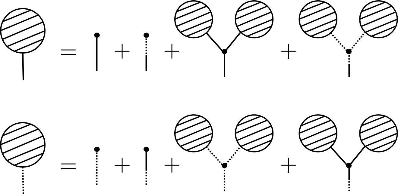
Using the graphical expressions shown in Fig. 2, one can write the equations defining the summations over all connected planar, rooted tree graphs denoted by :
| (3.8) | ||||
| (3.9) |
Solving (3.8) and (3.9) one obtains
| (3.10) |
The quadratic terms in the potential (3.7) produce “dressed” propagators which are alternatively obtained by summing all connected planar, rooted tree graphs attached to the propagators generated by the potential (3.4):
| (3.11) |
| (3.12) |
where indices of matrices are omitted. A graph obtained by integrating out all tree graphs is depicted in the right-hand side of Fig. 1, which is called a cubic “skeleton” graph [25]. Rescaling the matrices,
| (3.13) |
one obtains the following potential:
| (3.14) |
where
| (3.15) |
As we have seen above, starting from the potential, , one can erase the linear terms by the linear transformation (3.5), which is equivalent to integrating out all connected planar, rooted tree graphs, and the parameter, , can be absorbed by rescaling the matrices (3.13) and redefinition of coupling constants (3.15), resulting in the potential, . When , the linear terms are not important in the sense that they do not alter the criticality obtained by Kazakov, but they become important when is small: Since the power of in a graph generated by the potential, , can be counted as where is the number of loops in a graph, if is small, then loops are suppressed and as a result the tree graphs would be dominant [25]. Therefore, one can expect that tuning , the criticality of the model defined by the partition function (3.3) is governed by that of trees. As argued in [28], the Ising model on branched polymers (connected tree graphs) can be critical only at the zero temperature, i.e. . In fact, the average number of vertices in a tree,
| (3.16) |
the average number of vertices in the dressed propagators, and ,
| (3.17) |
and the average number of vertices in the dressed propagators, and ,
| (3.18) |
all diverge at the critical point,
| (3.19) |
Here the average number of vertices is that of faces in dual triangulations.
Taking into account the observations above, one would expect that using the two-matrix model (3.3) the critical point of the Ising model on dynamical triangulations specified by the critical coupling constants, , in which fluctuations of both triangulations and Ising spins diverge can reach the critical point of the Ising model on branched polymers by tuning , which is characterised by .
3.2 Saddle-point analysis
In the following we will investigate the two-matrix integral (3.3) basically using the techniques established in [32]. Changing the variables again,
| (3.20) |
(3.3) becomes up to overall constant
| (3.21) |
where
| (3.22) |
Since the and are Haar measures on U(), one can diagonalise in such a way that
| (3.23) |
with U() and implementing the Gaussian integration with respect to , (3.21) becomes up to overall constant
| (3.24) |
where
| (3.25) |
In the large- limit, the saddle-point equation, , becomes
| (3.26) |
Following [33] we introduce the non-decreasing function :
| (3.27) |
Then the saddle-point equation (3.26) becomes the following integral equation:
| (3.28) |
where P denotes Cauchy’s principal value. It is natural to introduce the density of eigenvalues,
| (3.29) |
satisfying the normalisation condition:
| (3.30) |
in which we have assumed that eigenvalues are distributed within the real interval, . Based on the density (3.29), the saddle-point equation (3.28) can be written as
| (3.31) |
We introduce the resolvent of the matrix in the large- limit:
| (3.32) |
defined for complex outside the real interval, . By definition of Cauchy’s principal value, the saddle-point equation (3.31) can be written in terms of the resolvent (3.32) as
| (3.33) |
A polynomial solution to (3.33) is
| (3.34) |
We rewrite the saddle-point equation (3.33) in terms of
| (3.35) |
as
| (3.36) |
This homogeneous equation implies the structure of Riemann surface consisting of three sheets with square root branch cuts [32], and by definition of the eigenvalue distribution (3.30) there is a single square root branch cut, , on the sheet we are working on, called physical sheet.
Taking into account that for large , we obtain
| (3.37) |
3.3 Algebraic cubic equation
Using the resolvent (3.32) of the matrix , the saddle point equation (3.26) in the large- limit can be also written as follows:
| (3.38) |
where is a constant. In terms of (3.35), (3.38) can be recast in
| (3.39) |
where is a regular even function. As anticipated from the structure of Riemann surface, the saddle-point equation (3.39) can be written as an algebraic cubic equation multiplying by :
| (3.40) |
where is an even polynomial since is regular everywhere [32]. Introducing the following useful notation [32],
| (3.41) |
with , one notices
| (3.42) |
then can be written in terms of as
| (3.43) |
Using the notation (3.41) we can express the algebraic cubic equation (3.40) as
| (3.44) |
As well the homogeneous equation (3.36) has the following alternative form:
| (3.45) |
Assuming (3.45) one can recover the homogeneous equation (3.36).
4 Perturbations around critical point
The analytic structure of the resolvent (or equivalently that of ) can change when some zeros of in (3.50) coincide; this change of analytic structure would happen if coupling constants reach their radius of convergence for the resolvent. The corresponding coupling constants are critical coupling constants. In the following we will find one-parameter family of the critical coupling constants, and , on which interactions among triangulations and Ising spins become strongest, and then tune to .
Since on the physical sheet we have assumed that there exists a single square root branch cut, , we consider the confluence of one of the end points of the branch cut and the other zeros of , and . As investigated in [32] when is not zero, the confluence, , corresponds to the conventional critical point of one-matrix model around which one can take the continuum limit resulting in the quantised theory of pure gravity, and on the other hand, the confluence, , makes the Ising-spin fluctuations diverge. Therefore, the simultaneous confluence of two zero’s, , corresponds to the criticality associated with the quantised theory of gravity coupled to conformal matter with central charge being .
Let us consider the confluence, , and determine the corresponding generic form of . The critical solution satisfying can be determined by the following four conditions:
- 1.
There exists a single branch cut, , on the physical sheet.
- 2.
should satisfies the equation (3.45).
- 3.
The product, , is a polynomial.
- 4.
for large .
As a result, one obtains [32]
| (4.1) |
where is a constant to be determined. Accordingly, one finds
| (4.2) |
Comparing (4.2) with (3.50) under the condition , one can describe in terms of and :
| (4.3) |
The large- expansion of (4.1) becomes
| (4.4) |
Comparing the large- expansions, (4.4) and (3.49), one obtains a set of equations:
| (4.5) | ||||
| (4.6) | ||||
| (4.7) |
From the conditions, and , and the set of equations (4.5) - (4.7), one can find the region for to satisfy:
| (4.8) |
The following two critical behaviours can be expected [32] 66 6 One cannot consider since from (4.3) one has to choose as or , which are out of the range (4.8). :
- 1.
We don’t consider further confluence of zero and set by choosing (see (4.5)), which as a result “freezes” the Ising-spin degrees of freedom, resulting in the conventional criticality of the one-matrix model.
- 2.
We consider further confluence of zero such that , which can be realised by setting from (4.3). At this critical regime, interactions among triangulations and Ising spins become strongest.
The case above might look weird since although the critical condition, , means the divergent fluctuations of Ising spins, the conventional criticality of the one-matrix model can be reached. This might happen because fluctuations of Ising spins would be converted to those of triangulations by setting , which can be confirmed by the fact that the critical coupling constant associated with the case coincides with the conventional coupling constant of one-matrix model. In the following, let us check the two cases above for small .
4.1 Case with
4.2 Case with
We consider the set of equations, (4.5) - (4.7), with . From (4.7), one finds
| (4.13) |
From (4.5), (4.6) and (4.13), one obtains the equation which the critical satisfies
| (4.14) |
and
| (4.15) |
For a fixed , one can obtain the critical value of , , by solving (4.14); accordingly, critical value of and , and , can be obtained from (4.13) and (4.15), respectively. The solution to (4.14) in the regime, , is
| (4.16) |
where
| (4.17) |
The small- expansion of (4.16) is given as
| (4.18) |
where is the critical coupling of the Ising model on branched polymers defined in (3.19). Plugging (4.16) into (4.15), one obtains the critical value of :
| (4.19) |
Remembering that is related with the inverse temperature as one finds that the critical temperature reaches absolute zero as :
| (4.20) |
A plot of the critical line is given by Fig. 3.

5 Continuum limit
In Section 4, we have obtained the critical point at absolute zero as a critical end point of the two critical lines, (4.10) for and (4.16) for , as . Since when is small the two-matrix integral would be dominated by its “classical” value, one would expect that the potential term, , in the two-matrix integral (3.21), would be important in the continuum limit as opposed to the conventional continuum limit with being non-zero, meaning that the potential term would also scale non-trivially in the continuum limit. In order to make this point clear, we rewrite (3.21) as
| (5.1) |
where and are eigenvalues of the matrices, and , respectively, and
| (5.2) |
| (5.3) |
The form of (5.1) can be obtained by a change of variables in the Harish-Chandra-Itzykson-Zuber integral [34, 35]. In fact, the critical point at absolute zero can be obtained in such a way that the first and the second derivatives of the potential vanish,
| (5.4) |
where
| (5.5) |
This means that if we assume that the eigenvalues scale as which is the lattice spacing since all eigenvalues approach zero as , then the potential would scale as . This observation motivates us to take the continuum limit at the level of the two-matrix integral (3.21), resulting in the continuum matrix model, as done in [24] for the Hermitian one-matrix model case, instead of determining the continuum form of the resolvent directly. In fact in the case of the Hermitian one-matrix model, it has been shown in [24] that the continuum matrix model can correctly reproduce the resolvent of generalised CDT at least in the large- limit. Taking into account the expected scaling of the potential, , it would be natural to set the scaling of as
| (5.6) |
where is the renormalised coupling constant. In the following, we will take the continuum limit of the partition function (3.21) around the two critical lines close to the critical end point (5.5).
5.1 Case with
Setting , we consider the continuum limit around the critical line (4.10) close to the critical end point (5.5). As examined in the Hermitian one-matrix model in [24], the corresponding continuum theory should be generalised CDT; we will check if it is really the case. From (4.12), we tune the coupling constant as
| (5.7) |
where is the renormalised cosmological constant and is given by
| (5.8) |
and the scaling of is given by (5.6). Changing variables in (3.21),
| (5.9) |
and inserting (5.6) and (5.7) into the two-matrix integral (3.21), one obtains the following two-matrix model in the small- limit 77 7 In the large- limit, the model in the continuum limit (5.10) is equivalent to the one formulated in [36] based on a string field theory for CDT with extended interactions if we choose . :
| (5.10) |
where
| (5.11) |
In fact, the two-matrix integral (5.10) can be written as a product of two identical one-matrix integrals: Expressing and as linear combinations of new variables, ,
| (5.12) |
one finds
| (5.13) |
where
| (5.14) |
The matrix integral (5.14) is equivalent to the one introduced in [24], which gives the correct disk amplitude of generalised CDT in the large- limit. Therefore, as expected the continuum theory starting from the condition, , is essentially generalised CDT; the corresponding string susceptibility is known: [12].
5.2 Case with
In the case with , from (4.15) and (4.18) we tune the coupling constants as
| (5.15) | ||||
| (5.16) |
and the scaling of is given by (5.6). Similarly, changing the variables as (5.9) and inserting (5.6), (5.15) and (5.16) into (3.21), one obtains the following two-matrix model in the small- limit:
| (5.17) |
where
| (5.18) |
Changing variables,
| (5.19) |
one can rewrite the matrix integral (5.17) in a symmetric fashion up to overall constant:
| (5.20) |
where
| (5.21) |
with
| (5.22) |
From this expression, it is apparent that the interaction among and vanishes when .
In the limits, and , the two-matrix integral (5.20) would be dominated by the saddle point, , and the resolvent of would reduce to that of CDT (up to redefinition of the renormalised cosmological constant), and therefore the string susceptibility is . This is natural because the model given by and generalised CDT originate with the same critical point where is zero.
6 Discussion
In this paper, we have reconsidered the criticality of the Ising model on d DT with the introduction of the loop-counting parameter, , and the linear terms. As a result, we have shown that the conventional non-zero critical temperature of the Ising model dressed by quantum gravity can reach absolute zero as . This happens because tuning , the criticality would be governed by that of the Ising model on branched polymers, which becomes critical only at the zero temperature. Also, we have identified the continuum theory defined around the critical end point (at absolute zero) of the critical line with , which can be described by the non-trivial continuum two-matrix model (5.20).
We elaborate how configurations of triangulations and Ising spins can be affected by the critical point at absolute zero. Firstly let us review what happens at the non-zero critical temperature. When the temperature is lower than the critical temperature, Ising spins are on average aligned in the same direction, i.e. magnetised, and triangulations are not affected by Ising spins. On the other hand, when the temperature is higher than the critical temperature, it is favourable for Ising spins to be randomly oriented since the entropy of the Ising model would be more important than the magnetic energy in this regime, and therefore triangulations are again independent of the Ising-spin degrees of freedom. It is known that interactions among triangulations and Ising spins become strongest at the critical temperature. When approaching to the critical temperature fluctuations of Ising spins are getting divergent, which change triangulations in such a way that the length of the boundary of clusters of Ising spins aligned in the same direction gets shorter and eventually becomes the length being of order of the lattice spacing on average around the critical temperature. This is because the magnetic energy, energy needed to flip Ising spins, would be proportional to the length of the cluster of Ising spins and the shorter the length is, the more easily Ising spins fluctuate (see e.g. [7]). Therefore, on the critical line triangulations are changed by Ising spins into those consisting of the clusters of Ising spins connected by the minimum possible links called minimum neck baby universes (abbreviated mimbu [29]). Around the critical line, one can define the continuum limit and the resulting field theory is known to be the quantised theory of two-dimensional Euclidean gravity coupled to conformal matter with central charge being [9], in which trees attached to ensembles are not important.
Decreasing along the vicinity of the critical line, mimbu’s would tend to “slim down” to form trees on average. At the critical end point, , typical geometries would become branched polymers. Around the critical point at absolute zero two kinds of continuum limit would be considered depending on how we go away from it since two kinds of critical lines specified by (4.10) and (4.16), respectively, meet at the same critical point. The first possibility is to go away along the curve of pure gravity given by (4.12) on which the coupling constant is taken to be zero. The corresponding continuum theory is generalised CDT as shown in 5.1. Another possibility is to be away along the curve given by (4.18) with non-zero . As shown in 5.2 the corresponding continuum theory would be the one defined by the two-matrix model (5.20) in the large- limit, in which divergent fluctuations of Ising spins are taken into account, but its physical properties would be closer to those of generalised CDT than the Liouville quantum gravity coupled to conformal matter with central charge being since the two continuum theories originate with the same critical point.
Here we emphasise that the continuum limit discussed in this paper is nothing to do with that of the Ising model on (generalised) CDT in which Ising spins are put in the centre of triangles: Although when typical geometries become trees (with finite number of loops) which can be mapped to ensembles of (generalised) CDT, after mapping to (generalised) CDT Ising spins are not placed in the centre of triangles.
As conjectured in [14], the quantised theory of the non-projectable Hořava-Lifshitz gravity in two dimensions would be generalised CDT because of the “many” fingered proper time of Wheeler (for the detail, see Discussion in [14]). Similarly we conjecture that the quantised theory of the non-projectable Hořava-Lifshitz gravity coupled to fermions in two dimensions is the model defined by the continuum two-matrix model (5.20) at least in the large- limit.
It is important to compute the critical exponents around by introducing an external magnetic filed as done in [10] when , which would tell us the effects caused by back-reactions of triangulations on Ising-spin configurations.
Since the Ising model on d DT can be considered as the O()-matrix model [32], it would be natural to consider the general O()-matrix model with the introduction of and the linear terms, and argue the critical points when .
It would be possible to describe the model defined by the two-matrix model (5.20) in terms of string field theory as done for generalised CDT in [23].
The critical point at absolute zero obtained in this paper might be interpreted as a quantum critical point since even though the Ising model we consider is classical, quantum fluctuations of triangulations would allow us to reduce the critical temperature to absolute zero. The relation to the quantum criticality would be worthwhile to examine in detail, which might lead to further understanding of two-dimensional quantum gravity coupled to matter, in which the continuum two-matrix model (5.20) might play a key role.
Acknowledgement
YS would like to thank Jan Ambjørn, Dario Benedetti, Timothy Budd, Bergfinnur Durhuus, Benjo Fraser, Masafumi Fukuma, Kazuki Hasebe, Shinji Hirano, Hiroshi Isono, Daisuke Kadoh, Issaku Kanamori, Noboru Kawamoto, Rob Knoops, Luca Lionni, Antonino Marcianò, So Matsuura, Shiraz Minwalla, Takeshi Morita, Shinsuke M. Nishigaki, Jun Nishimura, Naoki Sasakura, Hidehiko Shimada, Fumihiko Sugino, Seiji Terashima, Asato Tsuchiya, Naoya Umeda and Yoshiyuki Watabiki for encouragement, discussions and comments. YS visited LPTHE, Paris, France, the Niels Bohr Institute, Copenhagen, Denmark and University of the Witwatersrand, Johannesburg, South Africa where part of this work was done. He would like to thank all the members there for the kind hospitality. The work of YS is funded under CUniverse research promotion project by Chulalongkorn University (grant reference CUAASC).
References
- [1] J. Ambjørn, B. Durhuus and J. Frohlich, “Diseases of Triangulated Random Surface Models, and Possible Cures,” Nucl. Phys. B 257 (1985) 433. doi:10.1016/0550-3213(85)90356-6
- [2] J. Ambjørn, B. Durhuus, J. Frohlich and P. Orland, “The Appearance of Critical Dimensions in Regulated String Theories,” Nucl. Phys. B 270 (1986) 457. doi:10.1016/0550-3213(86)90563-8
- [3] F. David, “Planar Diagrams, Two-Dimensional Lattice Gravity and Surface Models,” Nucl. Phys. B 257 (1985) 45. doi:10.1016/0550-3213(85)90335-9
- [4] A. Billoire and F. David, “Microcanonical Simulations of Randomly Triangulated Planar Random Surfaces,” Phys. Lett. 168B (1986) 279. doi:10.1016/0370-2693(86)90979-2
- [5] V. A. Kazakov, A. A. Migdal and I. K. Kostov, “Critical Properties of Randomly Triangulated Planar Random Surfaces,” Phys. Lett. 157B (1985) 295. doi:10.1016/0370-2693(85)90669-0
- [6] D. V. Boulatov, V. A. Kazakov, I. K. Kostov and A. A. Migdal, “Analytical and Numerical Study of the Model of Dynamically Triangulated Random Surfaces,” Nucl. Phys. B 275 (1986) 641. doi:10.1016/0550-3213(86)90578-X
- [7] J. Ambjørn, B. Durhuus and T. Jonsson, “Quantum Geometry : A Statistical Field Theory Approach,” Cambridge Monographs on Mathematical Physics, Cambridge University Press, Cambridge, 1997.
- [8] P. Di Francesco, P. H. Ginsparg and J. Zinn-Justin, “2-D Gravity and random matrices,” Phys. Rept. 254 (1995) 1 doi:10.1016/0370-1573(94)00084-G [hep-th/9306153].
- [9] V. A. Kazakov, “Ising model on a dynamical planar random lattice: Exact solution,” Phys. Lett. A 119 (1986) 140.
- [10] D. V. Boulatov and V. A. Kazakov, “The Ising Model on Random Planar Lattice: The Structure of Phase Transition and the Exact Critical Exponents,” Phys. Lett. B 186 (1987) 379. doi:10.1016/0370-2693(87)90312-1 [11]
- [11] V. G. Knizhnik, A. M. Polyakov and A. B. Zamolodchikov, “Fractal Structure of 2D Quantum Gravity,” Mod. Phys. Lett. A 3 (1988) 819. doi:10.1142/S0217732388000982
- [12] J. Ambjørn and R. Loll, “Nonperturbative Lorentzian quantum gravity, causality and topology change,” Nucl. Phys. B 536 (1998) 407 doi:10.1016/S0550-3213(98)00692-0 [hep-th/9805108].
- [13] J. Ambjørn, A. Goerlich, J. Jurkiewicz and R. Loll, “Nonperturbative Quantum Gravity,” Phys. Rept. 519 (2012) 127 doi:10.1016/j.physrep.2012.03.007 [arXiv:1203.3591 [hep-th]].
- [14] J. Ambjørn, L. Glaser, Y. Sato and Y. Watabiki, “2d CDT is 2d Hořava-Lifshitz quantum gravity,” Phys. Lett. B 722 (2013) 172 doi:10.1016/j.physletb.2013.04.006 [arXiv:1302.6359 [hep-th]].
- [15] J. Ambjørn, K. N. Anagnostopoulos and R. Loll, “A New perspective on matter coupling in 2-D quantum gravity,” Phys. Rev. D 60 (1999) 104035 doi:10.1103/PhysRevD.60.104035 [hep-th/9904012].
- [16] J. Ambjørn, K. N. Anagnostopoulos and R. Loll, “Crossing the c = 1 barrier in 2-D Lorentzian quantum gravity,” Phys. Rev. D 61 (2000) 044010 doi:10.1103/PhysRevD.61.044010 [hep-lat/9909129].
- [17] P. Di Francesco, E. Guitter and C. Kristjansen, “Integrable 2-D Lorentzian gravity and random walks,” Nucl. Phys. B 567 (2000) 515 doi:10.1016/S0550-3213(99)00661-6 [hep-th/9907084].
- [18] V. Malyshev, A. Yambartsev and A. Zamyatin, “Two-dimensional Lorentzian models,” Mosc. Math. J., 1(3):439-456, 2001.
- [19] M. Krikun and A. Yambartsev, “Phase transition for the Ising model on the critical Lorentzian triangulation,” J. Statist. Phys. 148 (2012) 422 [arXiv:0810.2182[math.PR]].
- [20] B. Durhuus, T. Jonsson and J. F. Wheater, “On the spectral dimension of causal triangulations,” J. Statist. Phys. 139 (2010) 859 doi:10.1007/s10955-010-9968-x [arXiv:0908.3643 [math-ph]].
- [21] J. Ambjørn and T. G. Budd, “Trees and spatial topology change in CDT,” J. Phys. A: Math. Theor. 46 (2013) 315201 doi:10.1088/1751-8113/46/31/315201 [arXiv:1302.1763 [hep-th]].
- [22] J. Ambjørn, R. Loll, W. Westra and S. Zohren, “Putting a cap on causality violations in CDT,” JHEP 0712 (2007) 017 doi:10.1088/1126-6708/2007/12/017 [arXiv:0709.2784 [gr-qc]].
- [23] J. Ambjørn, R. Loll, Y. Watabiki, W. Westra and S. Zohren, “A String Field Theory based on Causal Dynamical Triangulations,” JHEP 0805 (2008) 032 doi:10.1088/1126-6708/2008/05/032 [arXiv:0802.0719 [hep-th]].
- [24] J. Ambjørn, R. Loll, Y. Watabiki, W. Westra and S. Zohren, “A New continuum limit of matrix models,” Phys. Lett. B 670 (2008) 224 doi:10.1016/j.physletb.2008.11.003 [arXiv:0810.2408 [hep-th]].
- [25] J. Ambjørn, T. Budd and Y. Watabiki, “Scale-dependent Hausdorff dimensions in 2d gravity,” Phys. Lett. B 736 (2014) 339 doi:10.1016/j.physletb.2014.07.047 [arXiv:1406.6251 [hep-th]].
- [26] J. Ambjørn, L. Glaser, A. Gorlich and Y. Sato, “New multicritical matrix models and multicritical 2d CDT,” Phys. Lett. B 712 (2012) 109 doi:10.1016/j.physletb.2012.04.047 [arXiv:1202.4435 [hep-th]].
- [27] M. R. Atkin and S. Zohren, “On the Quantum Geometry of Multi-critical CDT,” JHEP 1211 (2012) 037 doi:10.1007/JHEP11(2012)037 [arXiv:1203.5034 [hep-th]].
- [28] J. Ambjørn, B. Durhuus, T. Jonsson and G. Thorleifsson, “Matter fields with coupled to -d gravity,” Nucl. Phys. B 398 (1993) 568 doi:10.1016/0550-3213(93)90604-N [hep-th/9208030].
- [29] S. Jain and S. D. Mathur, “World sheet geometry and baby universes in 2-D quantum gravity,” Phys. Lett. B 286 (1992) 239 doi:10.1016/0370-2693(92)91769-6 [hep-th/9204017].
- [30] J. Ambjørn, S. Jain and G. Thorleifsson, “Baby universes in 2-d quantum gravity,” Phys. Lett. B 307 (1993) 34 doi:10.1016/0370-2693(93)90188-N [hep-th/9303149].
- [31] J. Ambjørn, S. Jain, J. Jurkiewicz and C. F. Kristjansen, “Observing 4-d baby universes in quantum gravity,” Phys. Lett. B 305 (1993) 208 doi:10.1016/0370-2693(93)90109-U [hep-th/9303041].
- [32] B. Eynard and J. Zinn-Justin, “The O(n) model on a random surface: Critical points and large order behavior,” Nucl. Phys. B 386 (1992) 558 [hep-th/9204082].
- [33] E. Brezin, C. Itzykson, G. Parisi and J. B. Zuber, “Planar Diagrams,” Commun. Math. Phys. 59 (1978) 35. doi:10.1007/BF01614153
- [34] Harish-Chandra, “Differential operators on a semisimple Lie algebra,” Amer. J. Math. 79 (1957) 87.
- [35] C. Itzykson and J. B. Zuber, “The Planar Approximation. 2.,” J. Math. Phys. 21 (1980) 411 doi:10.1063/1.524438.
- [36] H. Fuji, Y. Sato and Y. Watabiki, “Causal Dynamical Triangulation with Extended Interactions in 1+1 Dimensions,” Phys. Lett. B 704 (2011) 582 doi:10.1016/j.physletb.2011.09.032 [arXiv:1108.0552 [hep-th]].