Elliptic operators with honeycomb symmetry: Dirac points, Edge States and Applications to Photonic Graphene

Motivated by the novel and subtle properties of electronic waves in graphene [34], there has been very wide interest in the propagation of waves in two-dimensional structures having the symmetries of a hexagonal tiling of the plane and its applications to electromagnetic and other types of waves; see, for example, [78, 75, 44, 60, 83, 82]. Such physical systems have been dubbed artificial graphene. The present article is motivated by photonic graphene; the propagation of waves governed by the two-dimensional Maxwell equations in honeycomb media.

Among the remarkable properties of graphene (actual and artificial) being intensively explored in the fundamental and applied scientific communities are the existence of Dirac points [61, 67, 80, 26, 29, 8] (conical points at the intersections between dispersion surfaces), the implied wave-packet (quasi-particle) dynamics of states which are spectrally localized near Dirac points [69, 1, 27], and topologically protected edge states [37, 74, 61, 19, 73, 70, 57, 15, 58, 24, 16, 28]. Conical singularities in dispersion relations and their consequences for wave propagation have a long history. For example, they are well-known to occur for spatially homogeneous anisotropic Maxwell’s equations; see [10] and references cited therein.

The goal of this paper is to investigate the phenomena of Dirac points, effective dynamics of wavepackets and the bifurcation theory of topologically protected edge states in the context of a class of elliptic partial differential operators, which incorporates important physical cases of electromagnetic propagation in honeycomb structures. Specifically we consider a class of periodic scalar divergence-form operators:

with structural assumptions on $A({\bf x})$, which we now discuss.

Introduce the following operations: $\mathcal{C}[f]({\bf x})=\overline{f({\bf x})},\$ $\mathcal{P}[f]({\bf x})=f(-{\bf x})$, and $\mathcal{R}[f]({\bf x})\equiv f(R^{*}{\bf x})$, where $R$ is the $120^{\circ}$ clockwise rotation matrix of vectors in the plane. For the bulk (unperturbed) structure, specified by a $2\times 2$ matrix function $A({\bf x})$, we assume the following properties:

1. (i)

   $A({\bf x})$ is periodic with respect to the equilateral triangular lattice, $\Lambda_{h}$; see Section 3.1.

2. (ii)

   ${\mathcal{L}^{A}}$ is self-adjoint and uniformly elliptic on $\mathbb{R}^{2}$,
   and with respect to some origin of coordinates:

3. (iii)

   ${\mathcal{L}^{A}}$ is $\mathcal{PC}-$ invariant; $\left[\mathcal{PC},{\mathcal{L}^{A}}\right]=0$, and

4. (iv)

   ${\mathcal{L}^{A}}$ is $\mathcal{R}-$ invariant; $\left[\mathcal{R},{\mathcal{L}^{A}}\right]=0$, where $[\mathcal{L}_{1},\mathcal{L}_{2}]=\mathcal{L}_{1}\mathcal{L}_{2}-\mathcal{L}_{2}\mathcal{L}_{1}$.

In this article we obtain results on:

1. 1.

   Dirac points (conical singularities) in the Floquet-Bloch dispersion surfaces associated with the eigenvalue problem ${\mathcal{L}^{A}}\psi=E\psi$; see (2.3).

2. 2.

   The non-persistence of Dirac points (opening of a local spectral gap) for the perturbed eigenvalue problem for the operator $\mathcal{L}^{A+\delta B}$, where $\delta\ll 1$ and $B({\bf x})$ breaks $\mathcal{P}-$ or $\mathcal{C}-$ invariance, and the persistence of Dirac points for small $\mathcal{P}\mathcal{C}-$ invariant perturbations.

3. 3.

   The bifurcation of topologically protected edge states from Dirac points upon introduction of a (non-compact) domain wall modulated periodic perturbation, $\mathcal{L}_{\rm dw}^{\delta}$, of ${\mathcal{L}^{A}}$; see (d) in Section 1.2.

Two examples in 2D electromagnetics which motivate our study of this class of operators, and to which our results apply, arise for Maxwell’s equations considered in (1) magneto-optic media and (2) in bi-anisotropic meta-materials.

We give a brief summary of our main results. Our approach makes use of and extends methods developed to treat the case of honeycomb Schrödinger operators [26, 27, 23, 24, 28, 25, 29].

1. 1.

   Characterization of honeycomb structured media: Theorem 3.1 and Corollary 1 characterize 2D honeycomb structured media, defined by the Hermitian operator ${\mathcal{L}^{A}}=-\nabla\cdot A({\bf x})\nabla$ (see (1.1)), where $A({\bf x})$ satisfies conditions (i)-(iv) above.

2. 2.

   Dirac points: Theorem 4.1 gives conditions for the existence of Dirac points at the vertices of the Brillouin zone, $\mathcal{B}_{h}$. Theorem 4.2 states that all sufficiently low-contrast honeycomb structures, for which a distinguished Fourier coefficient of the structure is non-zero, have Dirac points. Depending on the sign of this Fourier coefficient, these Dirac points occur either at intersections of the $1^{st}$ and $2^{nd}$ or $2^{nd}$ and $3^{rd}$ dispersion surfaces. Extension of these results to generic honeycomb structured media of arbitrary contrast, using the strategy of [26] (see also Appendix D of [25]) is discussed in Section 4.3. In Figure 1 we plot two dispersion surfaces for a honeycomb structured medium, $A({\bf x})$, which intersect at Dirac points for quasi-momenta located at the size vertices of the Brillouin zone.

   Remark 5 discusses the effective dynamics of wave-packets for initial data which are spectrally localized near Dirac points. The envelope of such wave-packets evolves slowly and on long time scales according to an effective massless Dirac equation.

   

3. 3.

   Non-persistence and persistence of Dirac points: Theorem 5.1 studies the instability of Dirac points under perturbations of honeycomb media, $-\nabla\cdot A\nabla\ \to\ -\nabla\cdot\ \left(\ A({\bf x})+\delta B({\bf x})\ \right)\nabla$ which break either $\mathcal{P}-$ or $\mathcal{C}-$ invariance; thus, $[\mathcal{PC},{\mathcal{L}^{B}}]\neq 0$. Here, $\mathcal{P}-$ refers to parity inversion, $f({\bf x})\mapsto\mathcal{P}[f]({\bf x})=f(-{\bf x})$ and $\mathcal{C}-$ refers to complex conjugation, $f({\bf x})\mapsto\mathcal{C}[f]({\bf x})=\overline{f({\bf x})}$. If $\mathcal{PC}-$ invariance is preserved, then the Dirac points persist, although their associated quasi-momenta may no longer be located on the vertices of the Brillouin Zone.

4. 4.

   Topologically protected edge states (Theorems 6.1 and 6.3): We consider a honeycomb structure perturbed by an edge, across which the structure is adiabatically modulated by a domain wall. ¹¹ 1 We comment briefly on the terms edge and edge state. An edge is frequently understood to mean an abrupt termination of bulk structure. The terms “edge” for a line-defect across which there is a change in a key characteristic of the structure, and “edge state” are also used in the physics literature; see, for example, [37, 74, 44]. The edge states we discuss are of the latter type.

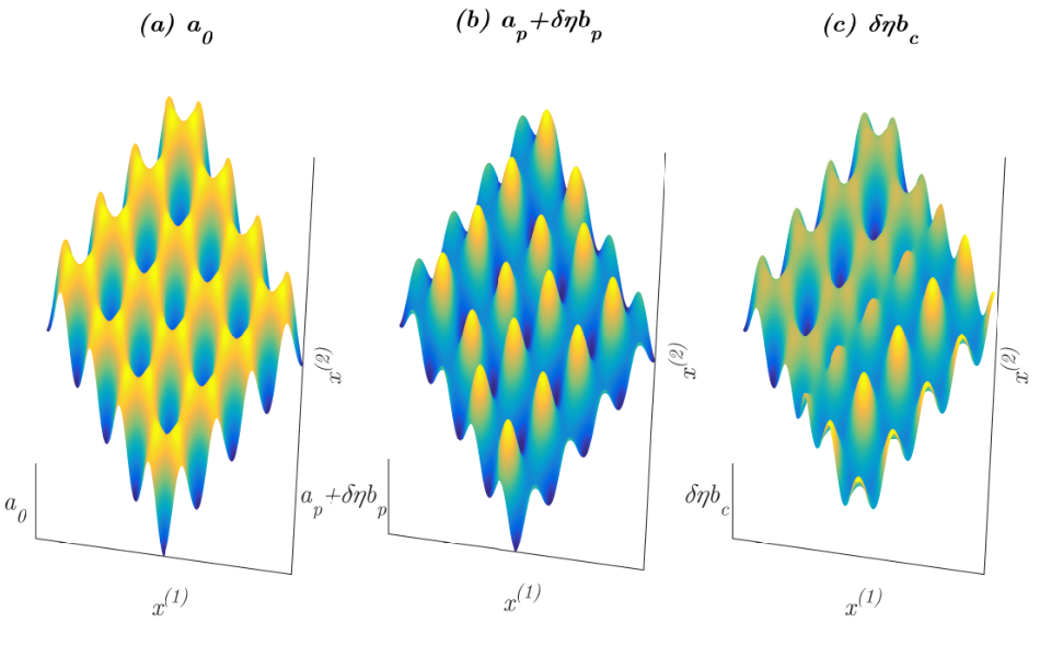
   Starting from a honeycomb operator with Dirac points, ${\mathcal{L}^{A}}$, we first consider operators $\mathcal{L}^{\delta}_{\pm\infty}=-\nabla\cdot\left[A({\bf x})\pm\delta\eta_{\infty}B({\bf x})\right]\nabla$. Here, $\delta$ is small non-zero real parameter, $\eta_{\infty}>0$, and $B({\bf x})$ breaks $\mathcal{PC}-$ invariance, i.e. $[\mathcal{PC},B]\neq 0$. It follows from (c) that the operators $\mathcal{L}^{\delta}_{\pm\infty}$ have a local spectral gap, i.e. a gap for quasi-momenta varying near Dirac points. Next, transverse to the line $\mathbb{R}{\bm{\mathfrak{v}}}_{1}$ in the lattice direction ${\bm{\mathfrak{v}}}_{1}\in\Lambda_{h}$, we interpolate between operators $\mathcal{L}^{\delta}_{\pm\infty}$ with a domain wall function $\eta(\zeta)$:

   $$\eta(0)=0,\ \ \eta(\zeta)\rightarrow\pm\eta_{\infty}\ \text{with}\ \ \eta_{\infty}>0\ \ \text{as}\ \ \zeta\rightarrow\pm\infty,$$

   (1.2)

   by introducing the operator

   $$\mathcal{L}_{\rm dw}^{(\delta)}\equiv-\nabla\cdot\left[A({\bf x})+\delta\eta(\delta{\bm{\mathfrak{K}}}_{2}\cdot{\bf x})B({\bf x})\right]\nabla\ .$$

   (1.3)

   Here, ${\bm{\mathfrak{K}}}_{2}\in\Lambda_{h}^{*}$ is such that ${\bm{\mathfrak{K}}}_{2}\cdot{\bm{\mathfrak{v}}}_{1}=0$. The constitutive matrix: $A({\bf x})+\delta\eta(\delta{\bm{\mathfrak{K}}}_{2}\cdot{\bf x})B({\bf x})$ defines a medium which is an interpolation (small and adiabatic), transverse to the line-defect / “edge” $\mathbb{R}{\bm{\mathfrak{v}}}_{1}$, between perturbed (“gapped ”) honeycomb structures.

   Associated with the ${\bf x}\mapsto{\bf x}+{\bm{\mathfrak{v}}}_{1}$ translation invariance of $\mathcal{L}_{\rm dw}^{(\delta)}$ is a parallel quasi-momentum, denoted ${k_{\parallel}}$. An edge state for parallel quasi-momentum, ${k_{\parallel}}$, is a non-trivial solution of the eigenvalue problem $\mathcal{L}_{\rm dw}^{(\delta)}\Psi=E\ \Psi$ such that $\Psi({\bf x}+{\bm{\mathfrak{v}}}_{1})=e^{i{k_{\parallel}}}\Psi({\bf x})$ and $\Psi({\bf x})\to 0$ as $|{\bm{\mathfrak{K}}}_{2}\cdot{\bf x}|\to\infty$. The edge state eigenvalue problem is naturally posed on $L^{2}(\Sigma)$, where $\Sigma=\mathbb{R}^{2}/\mathbb{Z}{\bm{\mathfrak{v}}}_{1}$ is a cylinder. Edge states are propagating (plane-wave like) parallel to the edge and are localized transverse to the edge.

   Theorem 6.1 presents the formal multiple scale expansion of such states. These modes bifurcate from the continuous spectrum at the Dirac point energy of the underlying, unperturbed ($\delta=0$) operator as the perturbation parameter $\delta$ is varied away from zero. The bifurcation of these modes is “topologically protected” in the sense that these modes persist in the presence of spatially localized (even large) perturbations of the domain-wall function, $\eta(\zeta)$.

   The rigorous formulation of Theorem 6.1 is given in Theorem 6.3. Section 6.4 contains a detailed sketch of the proof of Theorem 6.3, based on the corresponding result for a class of Schrödinger operators (see [28] and [25]). A central role is played by the spectral no-fold condition which is motivated and discussed. The validity of this condition for low contrast honeycomb structures for zigzag edges follows directly from the analysis for the corresponding Schrödinger operator case [28]. Figure 2 illustrates numerical computations of bifurcations of edge states.

   

5. 5.

   Group velocity properties of wavepackets concentrated along edges: Theorem 7.1 shows the existence of edge states for all ${k_{\parallel}}$ near ${k_{\parallel}}={\bf K}\cdot{\bm{\mathfrak{v}}}_{1}$ and ${k_{\parallel}}=-{\bf K}\cdot{\bm{\mathfrak{v}}}_{1}$. Taking a weighted and continuous superposition of such edge states in ${k_{\parallel}}$, yields fully localized wave-packets which are concentrated along the edge. The group velocity of these wave-packets is given by $\partial_{k_{\parallel}}E({k_{\parallel}})$ evaluated at ${k_{\parallel}}=\pm{\bf K}\cdot{\bm{\mathfrak{v}}}_{1}$.

6. 6.

   Unidirectional edge propagation in time-reversal invariant and $\mathcal{C}-$ breaking media: In Section A.4 we apply our results to the propagation of edge states in the two examples discussed in Section 1.1: (1) magneto-optic media, and (2) bi-anisotropic media; see also Appendix A. We consider the special cases where $\mathcal{PC}-$ invariance is broken by perturbations which are (a) $\mathcal{P}-$ invariant, but $\mathcal{C}-$ anti-symmetric, and (b) $\mathcal{C}-$ invariant, but $\mathcal{P}-$ anti-symmetric. In case (a), the families of edge states constructed are uni-directional, although Maxwell’s equations in this setting is time-reversal invariant (Section A.1); see the top panel of Figure 3. In case (b), the resulting edge states propagate bi-directionally; see the bottom panel of Figure 3.

   We remark that in [37, 74], which considers magneto-optic media, and [44], which considers bi-anisotropic media, it was assumed that the unperturbed bulk medium is isotropic ($A({\bf x})=a({\bf x})I_{{}_{2\times 2}}$). In this article we allow for a more general class of anisotropic media; see our definition of honeycomb structured medium in Section 3.4.

   

The existence of Dirac points for Schrödinger operators with generic honeycomb lattice potentials was proved in [26, 25]. Results for small amplitude potentials were obtained in [18, 36]. A group representation perspective on the existence and persistence of Dirac points is developed in [8]. The case where the potential is a superposition of delta function potentials centered on sites of the honeycomb structure is treated in [52]. The low-lying dispersion surfaces of honeycomb Schrödinger operators in the strong binding regime, where the potential is the superposition of a general class of atomic potential wells, and its relation to the tight-binding limit, was studied in [29]. Tight binding models have been studied extensively in the fundamental and applied physics and mathematics communities; see, for example, [6, 20, 2, 17].

A bifurcation theory of topologically protected bound states arising from domain wall perturbations of one-dimensional periodic Schrödinger operators with Dirac points (linear band crossings) is developed in [23, 25]. These results are applied to a photonic setting in [53] and [72, 71]. The bifurcation of topologically protected edge states arising from domain wall perturbations of two-dimensional honeycomb Schrödinger operators with Dirac points (conical band crossings) was studied in [28]; see also [24].

For an extensive discussion of Dirac points and edge states for nanotube structures in the context of quantum graphs, see [50] and [21]. For results on spectral gaps for elliptic problems modeling high contrast media, see [30, 31, 39, 40, 54, 55, 29]. For a general review of mathematical problems arising in photonics see, for example, [51].

The paper is structured as follows. In Section 2, we review the relevant spectral (Floquet-Bloch) theory and introduce the notions of $\mathcal{C}$, $\mathcal{P}$ and $\mathcal{R}$ invariance, associated with complex conjugation, parity and rotational symmetries. Section 3 introduces and characterizes honeycomb structured media via Fourier analysis. In Section 4 we discuss the notion of Dirac point in the band structure of the operator ${\mathcal{L}^{A}}$ and prove results for the cases of low-contrast and generic honeycomb structures. Section 5 discusses the stability of Dirac points against small perturbations which preserve $\mathcal{P}\circ\mathcal{C}$ symmetry and their instability when such symmetry is violated. In Section 6 we discuss the existence of topologically protected edge states. We first present the detailed formal multi-scale construction of such states and then give a detailed guide to adapting the proof for the case of Schrödinger operators [28] to the case of divergence form operators for honeycomb structured media. Note that results of this paper apply to large classes of complex-valued and anisotropic matrix-valued constitutive laws; see the examples arising in electromagnetics, discussed in Appendix A. Edge states are constructed for a range of parallel quasi-momenta ${k_{\parallel}}$. In Section 7 we discuss the edge state dispersion curves ${k_{\parallel}}\mapsto E({k_{\parallel}})$, which determine the propagation properties of edge-localized wave-packets; see, in particular, the discussion of group velocity in Subsection 7.1. Appendix A discusses Maxwell’s equations for bi-anisotropic media and the application of our general results to edge states and unidirectional edge-propagation in (1) magneto-optic and (2) bi-anisotropic media, both of which are time-reversal invariant. Appendix B provides a brief discussion of the numerical methods used in our computer simulations. Appendix C provides the specific potentials used in these simulations.

1. 1.

   $\Lambda_{h}\subset\mathbb{R}^{2}$ denotes the equilateral triangular lattice. $\Lambda_{h}^{*}\subset(\mathbb{R}^{2})^{*}=\mathbb{R}^{2}_{\bf k}$ denotes the dual lattice. ${\bf v}_{j},~j=1,2$ are the basis vectors of $\Lambda_{h}$. ${\bf k}_{l},~l=1,2$ are the dual basis vectors of $\Lambda_{h}^{*}$, chosen to satisfy ${\bf k}_{l}\cdot{\bf v}_{j}=2\pi\delta_{lj}$.

2. 2.

   ${\bm{\mathfrak{v}}}_{1}=a_{1}{\bf v}_{1}+a_{2}{\bf v}_{2}\in\Lambda_{h}$, $a_{1},a_{2}$ co-prime integers. The ${\bm{\mathfrak{v}}}_{1}$- edge is $\mathbb{R}{\bm{\mathfrak{v}}}_{1}$. ${\bm{\mathfrak{v}}}_{j},\ j=1,2$, is an alternate basis for $\Lambda_{h}$ with corresponding dual basis, ${\bm{\mathfrak{K}}}_{\ell},\ell=1,2$, satisfying ${\bm{\mathfrak{K}}}_{\ell}\cdot{\bm{\mathfrak{v}}}_{j}=2\pi\delta_{\ell j}$.

3. 3.

   For ${\bf m}=(m_{1},m_{2})\in\mathbb{Z}^{2}$, ${\bf m}\vec{\bf k}=m_{1}{\bf k}_{1}+m_{2}{\bf k}_{2}$.

4. 4.

   $\mathcal{B}$ denotes the Brillouin Zone, associated with $\Lambda_{h}$, shown in the right panel of Figure 4.

5. 5.

   $z\in\mathbb{C}\Rightarrow\overline{z}$ denotes the complex conjugate of $z$.

6. 6.

   $J=\begin{pmatrix}0&-1\\ 1&0\end{pmatrix}$ is the counterclockwise $90^{\circ}$ rotation matrix.

7. 7.

   ${\bf k}=(k^{(1)},k^{(2)})^{T}\in\mathbb{R}^{2}$ is represented in $\mathbb{C}$ by $\mathfrak{z}=k^{(1)}+ik^{(2)}$, and ${\bf k}_{\perp}\equiv J{\bf k}=(-k^{(2)},k^{(1)})^{T}$ is represented in $\mathbb{C}$ by $\mathfrak{z}_{\perp}=i\mathfrak{z}({\bf k})=\mathfrak{z}({\bf k}_{\perp})$. The corresponding points on the unit circle in $\mathbb{C}$ are denoted $\hat{\mathfrak{z}}({\bf k})$ and $\hat{\mathfrak{z}}({\bf k}_{\perp})$.

8. 8.

   $\nabla=(\partial_{x_{1}},\partial_{x_{2}})^{T}$.

9. 9.

   $\left\langle f,g\right\rangle_{D}=\int_{D}\overline{f}g$ is the $L^{2}(D)$ inner product. If the region of integration is not specified, it is assumed to be a choice of fundamental period cell, $\Omega$.

10. 10.

    Pauli matrices:

    $$\sigma_{1}=\begin{pmatrix}0&1\\ 1&0\end{pmatrix},\qquad\sigma_{2}=\begin{pmatrix}0&-i\\ i&0\end{pmatrix}=iJ,\qquad\sigma_{3}=\begin{pmatrix}1&0\\ 0&-1\end{pmatrix}.$$

11. 11.

    Unless otherwise specified, summation convention over repeated indices is assumed.

Let $\{{\bf v}_{1},{\bf v}_{2}\}$ be a linearly independent set in $\mathbb{R}^{2}$. The lattice generated by $\{{\bf v}_{1},{\bf v}_{2}\}$ is the subset of $\mathbb{R}^{2}$:

A choice of fundamental cell is the parallelogram:

The area of $\Omega$ is denoted $|\Omega|$.

The dual lattice, $\Lambda^{*}$, is defined to be

where ${\bf k}_{1}$ and ${\bf k}_{2}$ are dual lattice vectors, satisfying the reciprocal relations

We also introduce the (affine) lattice $\Lambda^{*}_{\bf k}$:

Let $L^{2}(\mathbb{R}^{2}/\Lambda)$ denote the space of $L^{2}_{loc}$ functions which are $\Lambda-$periodic, i.e. $f({\bf x}+{\bf v})=f({\bf x})$, for almost all ${\bf x}\in\mathbb{R}^{2}$ and all ${\bf v}\in\Lambda$. For ${\bf k}\in\mathbb{R}^{2}$, we denote by $L^{2}_{{\bf k}}$ the space of $L^{2}_{loc}$ functions such that $e^{-i{\bf k}\cdot{\bf x}}f({\bf x})\in L^{2}(\mathbb{R}^{2}/\Lambda)$, i.e. $f({\bf x}+{\bf v})=e^{i{\bf k}\cdot{\bf v}}f({\bf x}),\quad\text{for}\quad{\bf x}\in\mathbb{R}^{2},\ {\bf v}\in\Lambda$. Note that if ${\bf k}=0$, $L^{2}_{{\bf k}}$ reduces to $L^{2}(\mathbb{R}^{2}/\Lambda)$.

Let $f$ and $g$ in $L^{2}_{{\bf k}}$. Then, $\bar{f}g$ is locally integrable and $\Lambda-$periodic, and their inner product is naturally defined as

In a standard way, one can also introduce the Sobolev space $H^{s}_{{\bf k}}$.

Any $f\in L^{2}_{{\bf k}}$ has the Fourier expansion

We summarize definitions and results from the theory of self-adjoint, elliptic and periodic divergence form operators; see, for example, [47, 45, 46].

For each fixed ${\bf k}\in\mathbb{R}^{2}$, consider the $L^{2}_{\bf k}-$ Floquet-Bloch eigenvalue problem:

where ${\mathcal{L}^{A}}=-\nabla\cdot A\nabla$ was defined in (1.1). A solution of (2.3) is called a Floquet-Bloch state with quasi-momentum ${\bf k}$.

Since the ${\bf k}$-pseudo-periodic boundary condition in (2.3) is invariant under translation ${\bf k}\rightarrow{\bf k}+{{\bf k}}^{\prime}$ for any ${{\bf k}}^{\prime}\in\Lambda^{*}$, it suffices to consider ${\bf k}$ varying over a fundamental cell. A common choice is the Brillouin Zone $\mathcal{B}$, consisting of points ${\bf k}\in\mathbb{R}^{2}$ which are closer to the origin than to any other points in $\Lambda^{*}$; see Figure 4.

An alternative formulation of the eigenvalue problem (2.3) is obtained by setting $\Phi({\bf x})=e^{i{\bf k}\cdot{\bf x}}\phi({\bf x})$ for ${\bf k}\in\mathcal{B}$. Let

Then, (2.3) is equivalent to $\phi$ satisfying the periodic elliptic boundary value problem:

For each fixed ${\bf k}$, the eigenvalue problem (2.5) (equivalently (2.3)) has a discrete spectrum: $E_{1}({\bf k})\leq E_{2}({\bf k})\leq E_{3}({\bf k})\leq\cdots\leq E_{b}({\bf k})\leq\cdots$ with eigenpairs $(\phi_{b}({\bf x};{\bf k})$, $E_{b}({\bf k}))$, $b\geq 1$. The set $\left\{\phi_{b}({\bf x};{\bf k}):b\geq 1\right\}$ can be taken to be a complete and orthonormal set in $L^{2}(\mathbb{R}^{2}/\Lambda)$.

The mappings ${\bf k}\mapsto E_{b}({\bf k})$ are called band dispersion functions. They are Lipschitz-continuous, see, for example, [7, 47, 45, 46] and Appendix A of [27]. As ${\bf k}$ varies over $\mathcal{B}$, each function $E_{b}({\bf k})$ sweeps out a closed real interval. The union over $b\geq 1$ of these closed intervals is precisely the $L^{2}(\mathbb{R}^{2})$-spectrum of $\mathcal{L}^{A}$. Furthermore, the set $\left\{\Phi_{b}({\bf x};{\bf k})\right\}_{b\geq 1,{\bf k}\in\mathcal{B}}$ is complete in $L^{2}(\mathbb{R}^{2})$:

where the sum converges in the $L^{2}$ norm.

In this section we introduce terminology for discussing the symmetry properties of $A({\bf x})$ and ${\mathcal{L}^{A}}$. Let $g({\bf x})$ denote a function defined on $\mathbb{R}^{2}$.

$\mathcal{C}-$ invariance: The function $g({\bf x})$ is $\mathcal{C}-$ invariant if

for all ${\bf x}\in\mathbb{R}^{2}$.

$\mathcal{P}-$ invariance: The function $g({\bf x})$ is $\mathcal{P}-$ (or parity-inversion) invariant with respect to ${\bf x}_{0}\in\mathbb{R}^{2}$ if

for all ${\bf x}\in\mathbb{R}^{2}$.

$\mathcal{R}-$ invariance: The function $g({\bf x})$ is $\mathcal{R}-$ (or $120^{\circ}$- rotationally) invariant with respect to ${\bf x}_{0}\in\mathbb{R}^{2}$ if

for all ${\bf x}\in\mathbb{R}^{2}$. Here, ${\bf x}\mapsto R{\bf x}$ is the mapping on $\mathbb{R}^{2}$ which rotates a vector clockwise by $120^{\circ}$ ($2\pi/3$) about ${\bf x}={\bf 0}$:

For later use, we record the eigenvalues and a choice of normalized eigenvectors of $R$:

We say the operator $L$ with domain $D(L)\subset D(\mathcal{S})$, is $\mathcal{S}-$ invariant if the commutator $[\mathcal{S},L]\equiv\mathcal{S}L-L\mathcal{S}$ vanishes on $D(L)$.

In this section, we specialize the results of the previous section to the triangular lattice, $\Lambda_{h}$. Introduce the lattice

with lattice basis vectors

The dual lattice

is spanned by the dual basis vectors

see Figure 4. Note ${\bf k}_{l}\cdot{\bf v}_{m}=2\pi\delta_{lm}$, $l,m=1,2$.

The following proposition characterizes the high-symmetry points of the Brillouin Zone, $\mathcal{B}$.

The set of six vertices of $\mathcal{B}_{h}$ is invariant under $R$ and decomposes into the two subsets: the ${\bf K}\,\,\text{type-points:}\ {\bf K},\ R{\bf K}={\bf K}+{\bf k}_{2},\ R^{2}{\bf K}={\bf K}-{\bf k}_{1}$ and the ${\bf K}^{\prime}\,\,\text{type-points:}\ {\bf K}^{\prime},\ R{\bf K}^{\prime}={\bf K}-{\bf k}_{2},\ R^{2}{\bf K}^{\prime}={\bf K}^{\prime}+{\bf k}_{1}$. We note for future reference, the action of $R$ on ${\bf k}_{1}$ and ${\bf k}_{2}$:

We focus on the vertices of $\mathcal{B}_{h}$. Consider such a vertex, ${\bf K}_{\star}$. If $f$ is ${\bf K}_{\star}-$ pseudo-periodic, it is easy to check that $\mathcal{R}[f]$ is also ${\bf K}_{\star}-$ pseudo-periodic and that $\mathcal{R}$ is an isomorphism of $L^{2}_{{\bf K}_{\star}}$. Furthermore, $\mathcal{R}$ is unitary with eigenvalues $1$, $\tau$ and $\bar{\tau}$, where $\tau=\exp(2\pi i/3)$. It is therefore natural to split $L^{2}_{{\bf K}_{\star}}$ into the direct (orthogonal) sum:

where the summand subspaces are given by:

Let $A({\bf x})$ be a smooth $\Lambda_{h}-$ periodic and Hermitian matrix function, for which ${\mathcal{L}^{A}}=-\nabla\cdot A\nabla$ is elliptic in the sense of Assumption 1 of Section 2.2. In this section we derive further conditions on $A({\bf x})$ which ensure that ${\mathcal{L}^{A}}$ is $\mathcal{PC}-$ invariant and $\mathcal{R}-$ invariant.

We make use of the following general result. Let $O$ denote a real orthogonal matrix and define

The proof of Theorem 3.1 makes use of the following basic lemma:

We now turn to the proof of Theorem 3.1.

Recall that $R$ denotes the $120^{\circ}$ rotation matrix (2.7) and the mapping $\mathcal{R}:g({\bf x})\mapsto g(R^{*}{\bf x})$. The bulk structures we consider in this article, modeled by the operator ${\mathcal{L}^{A}}=-\nabla\cdot A\nabla$ are assumed to satisfy:

1. 1.

   ${\mathcal{L}^{A}}$ self-adjoint and elliptic. Hence, $A^{\dagger}=A$ and ellipticity condition $(A_{3})$ of Assumption 1 holds.

2. 2.

   $A({\bf x}+{\bf v})=A({\bf x})$ for all ${\bf x}\in\mathbb{R}^{2}$ and ${\bf v}\in\Lambda_{h}$.

3. 3.

   $[\mathcal{PC},{\mathcal{L}^{A}}]=0$ and hence $\overline{A(-{\bf x})}=A({\bf x})$, by Theorem 3.1 part 1.

4. 4.

   $[\mathcal{R},{\mathcal{L}^{A}}]=0$ and hence $A(R^{*}{\bf x})=R^{*}A({\bf x})R$, by Theorem 3.1 part 2.

References

• Ablowitz et al. (2009) M. J. Ablowitz, S. D. Nixon, and Y. Zhu Conical diffraction in honeycomb lattices. Physical Review A 79 (5), pp. 053830. Cited by: §1.1.
• Ablowitz et al. (2012) M. J. Ablowitz, C. W. Curtis, and Y. Zhu On tight-binding approximations in optical lattices. Studies in Applied Mathematics 129 (4), pp. 362–388. Cited by: §1.3.
• Allaire et al. (2011) G. Allaire, M. Palombaro, and J. Rauch Diffractive geometric optics for Bloch wave packets. Arch. Rat. Mech. Anal. 202 (2), pp. 373–426. Cited by: Remark 5.
• Allaire and Piatnitski (2005) G. Allaire and A. Piatnitski Homogenization of the Schrödinger equation and effective mass theorems. Comm. Math. Phys. 258 (1), pp. 1–22. External Links: ISSN 0010-3616, Link, Review MathReviews Cited by: Remark 5.
• Ando (2013) Y. Ando Topological insulator materials. Journal of the Physical Society of Japan 82 (10), pp. 102001. Cited by: §7.1.
• Ashcroft and Mermin (1976) N. W. Ashcroft and N. D. Mermin Solid State Physics. Harcourt, Orlando, FL (German). External Links: ISBN 3-486-57720-4/hbk Cited by: §1.3, Remark 5.
• Avron and Simon (1978) J. Avron and B. Simon Analytic properties of band functions. Ann. Phys. 110, pp. 85–101. Cited by: §2.2.
• Berkolaiko and Comech (1412) G. Berkolaiko and A. Comech Symmetry and Dirac points in graphene spectrum. Journal of Spectral Theory. Cited by: §1.1, §1.3, §4.2, §5.
• Bernevig and Hughes (2013) B. A. Bernevig and T. L. Hughes Topological insulators and topological superconductors. Princeton University Press, Princeton. Cited by: §7.1.
• Berry and Jeffrey (2007) M.V. Berry and M.R. Jeffrey Conical diffraction: hamilton’s diabolical point at the heart of crystal optics. In Progress in optics, E. Wolf (Ed.), Vol. 50. Cited by: §1.1.
• Birman and Suslina (1999) M. Sh. Birman and T. A. Suslina Two-dimensional periodic pauli operator. the effective masses at the lower edge of the spectrum. In Math. results in quantum mechanics, Oper. Theory Adv. Appl., Vol. 108, Basel, pp. 13–31. Cited by: Remark 5.
• Birman and Suslina (2001) M. Sh. Birman and T. A. Suslina Threshold effects near the lower edge of the spectrum for periodic differential operators of mathematical physics. In Systems, approximation, singular integral operators, and related topics, Oper. Theory Adv. and Appl., Vol. 129, Basel, pp. 71–107. Cited by: Remark 5.
• Birman and Suslina (2003) M. Sh. Birman and T. A. Suslina Periodic differential operators of the second order. threshold properties and homogenization. Algebra i Analyz 15 (2), pp. 1–108. Cited by: Remark 5.
• Birman and Suslina (2006) M. Sh. Birman and T. A. Suslina Homogenization of a multidimensional periodic elliptic operatorz in a neighborhood of the edge of internal gap. J. Math. Sci. 136 (2), pp. 3682–3690. Cited by: Remark 5.
• Chen et al. (2014) W. Chen, S. Jiang, X. Chen, B. Zhu, L. Zhou, J. Dong, and C. T. Chan Experimental realization of photonic topological insulator in a uniaxial metacrystal waveguide. Nature communications 5. Cited by: §1.1.
• Cheng et al. (2016) X. Cheng, C. Jouvaud, X. Ni, S. H. Mousavi, A. Z. Genack, and A. B. Khanikaev Robust reconfigurable electromagnetic pathways within a photonic topological insulator. Nature materials. Cited by: §1.1.
• Craster (2014) M. M. R. V. Craster Homogenization for hexagonal lattices and honeycomb structures. Q. Jl. Mech. Appl. Math.. Cited by: §1.3.
• de Verdiere (1991) Y. C. de Verdiere Sur les singularites de van hove generiques. Memoires de la S. M. F. serie 2 46, pp. 99–109. Cited by: §1.3.
• Delplace et al. (2011) P. Delplace, D. Ullmo, and G. Montambaux Zak phase and the existence of edge states in graphene. Physical Review B 84 (19), pp. 195452. Cited by: §1.1.
• Dimassi and Sjoestrand (1999) M. Dimassi and J. Sjoestrand Spectral asymptotics in the semi-classical limit. London Mathematical Society Lecture Note Series, Vol. 268, Cambridge University Press. Cited by: §1.3.
• Do and Kuchment (2013) N. T. Do and P. Kuchment Quantum graph spectra of a graphyne structure. Nanoscale Systems: Mathematical Modeling, Theory and Applications 2, pp. 107–123. Cited by: §1.3.
• Eastham (1973) M. S. P. Eastham The spectral theory of periodic differential equations. Scottish Academic Press, London. Cited by: §2.
• Fefferman et al. (2014) C. L. Fefferman, J. P. Lee-Thorp, and M. I. Weinstein Topologically protected states in one-dimensional continuous systems and dirac points. Proceedings of the National Academy of Sciences 111 (24), pp. 8759–8763. Cited by: §1.1, §1.2, §1.3, §6.4.
• Fefferman et al. (2016a) C. L. Fefferman, J. P. Lee-Thorp, and M. I. Weinstein Bifurcations of edge states – topologically protected and non-protected – in continuous 2d honeycomb structures. 2D Materials 3 (1), pp. 014008. Cited by: §1.1, §1.1, §1.2, §1.3, §6.
• Fefferman et al. (2017) C. L. Fefferman, J. P. Lee-Thorp, and M. I. Weinstein Topologically protected states in one-dimensional systems. Memoirs of the American Mathematical Society 247 (1173). Cited by: item 2, item 4, §1.1, §1.2, §1.3, §1.3, §4.3, §4.3, §6.4.
• Fefferman and Weinstein (2012) C. L. Fefferman and M. I. Weinstein Honeycomb lattice potentials and dirac points. Journal of the American Mathematical Society 25 (4), pp. 1169–1220. Cited by: item 2, §1.1, §1.2, §1.3, §3.4, §4.1, §4.2, §4.3, §4.3, §5.2, §5, §5, Proof, Proof, Remark 7.
• Fefferman and Weinstein (2014) C. L. Fefferman and M. I. Weinstein Wave packets in honeycomb structures and two-dimensional dirac equations. Communications in Mathematical Physics 326 (1), pp. 251–286. Cited by: §1.1, §1.2, §2.2, Remark 5.
• Fefferman et al. (2016b) C.L. Fefferman, J.P. Lee-Thorp, and M.I. Weinstein Edge states in honeycomb structures. Ann. PDE 2 (12). Cited by: item 4, §1.1, §1.1, §1.2, §1.3, §1.4, §6.4, §6.4, §6.4, §6.4, §6.4, §6, Proof, Remark 7.
• Fefferman et al. (2018) C.L. Fefferman, J.P. Lee-Thorp, and M.I. Weinstein Honeycomb Schroedinger operators in the strong-binding regime. Comm. Pure Appl. Math. 71 (6). Cited by: §1.1, §1.2, §1.3, §1.3, Remark 7.
• Figotin and Kuchment (1996a) A. Figotin and P. Kuchment Band-gap structure of spectra of periodic dielectric and acoustic media. I scalar model. SIAM J. Appl. Math. 56 (6), pp. 68–88. Cited by: §1.3.
• Figotin and Kuchment (1996b) A. Figotin and P. Kuchment Band-gap structure of spectra of periodic dielectric and acoustic media. I scalar model. SIAM J. Appl. Math. 56 (6), pp. 1561–1620. Cited by: §1.3.
• Fliss and Joly (2016) S. Fliss and P. Joly Solutions of the time-harmonic wave equation in periodic waveguides: asymptotic behaviour and radiation condition. Arch. Rat. Mech. Anal. 219 (1), pp. 349–386. Cited by: Appendix B.
• Fouque et al. (2007) J.-P. Fouque, J. Garnier, G. Papanicolaou, and K. Solna Wave propagation and time reversal in randomly layered media. Springer. Cited by: footnote 3.
• Geim and Novoselov (2007) A. K. Geim and K. S. Novoselov The rise of graphene. Nature materials 6 (3), pp. 183–191. Cited by: §1.1.
• Gesztesy et al. (2008) F. Gesztesy, Y. Latushkin, and K. Zumbrun Derivatives of (modified) fredholm determinants and stability of standing and traveling waves. J. Math. Pures Appl. 90, pp. 160–200. Cited by: §4.3.
• Grushin (2009) V. V. Grushin Multiparameter perturbation theory of Fredholm operators applied to Bloch functions. Mathematical Notes 86 (6), pp. 767–774. Cited by: §1.3.
• Haldane and Raghu (2008) F. D. M. Haldane and S. Raghu Possible realization of directional optical waveguides in photonic crystals with broken time-reversal symmetry. Physical review letters 100 (1), pp. 013904. Cited by: §A.4.1, §A.4, item 6, §1.1, §1.1, footnote 1.
• Hasan and Kane (2010) M. Z. Hasan and C. L. Kane Colloquium: topological insulators. Reviews of Modern Physics 82 (4), pp. 3045. Cited by: §7.1.
• Hempel and Lienau (2000) R. Hempel and K. Lienau Spectral properties of periodic media in the large coupling limit. Comm. PDE 25 (7-8), pp. 1445–1470. Cited by: §1.3.
• Hempel and Post (0207) R. Hempel and O. Post Spectral gaps for periodic elliptic operators with high contrast: an overview. Cited by: §1.3.
• Hoefer and Weinstein (2011) M. A. Hoefer and M. I. Weinstein Defect modes and homogenization of periodic schrödinger operators. SIAM Journal on Mathematical Analysis 43 (2), pp. 971–996. Cited by: Remark 5.
• Joannopoulos et al. (2011) J. D. Joannopoulos, S. G. Johnson, J. N. Winn, and R. D. Meade Photonic crystals: molding the flow of light. Princeton university press, Princeton. Cited by: Appendix A.
• Keller et al. (2018) R. T. Keller, J. Marzuola, B. Osting, and M. I. Weinstein Spectral band degeneracies of π2−\frac{\pi}{2}-rotationally invariant periodic Schrödinger operators. Cited by: Remark 5.
• Khanikaev et al. (2013) A. B. Khanikaev, S. H. Mousavi, W. Tse, M. Kargarian, A. H. MacDonald, and G. Shvets Photonic topological insulators. Nature materials 12 (3), pp. 233–239. Cited by: §A.2, §A.4.2, §A.4.2, §A.4.2, §A.4, item 6, §1.1, §1.1, footnote 1.
• Kuchment (2012) P. A. Kuchment Floquet theory for partial differential equations. Vol. 60, Birkhäuser, Basel. Cited by: §2.2, §2.2, §2.
• Kuchment (2015) P. A. Kuchment An overview of periodic elliptic operators. arXiv:1510.00971. Cited by: §2.2, §2.2, §2.
• Kuchment and Levendrskii (2001) P. Kuchment and S. Levendrskii On the structure of spectra of periodic elliptic operators. Trans. Amer. Math. Soc. 354, pp. 537–569. Cited by: §2.2, §2.2.
• Kuchment and Pinchover (2001) P. Kuchment and Y. Pinchover Integral representations and liouville theorems for solutions of periodic elliptic equations. J. Funct. Anal. 181, pp. 402–446. Cited by: Remark 5.
• Kuchment and Pinchover (2007) P. Kuchment and Y. Pinchover Liouville theorems and spectral edge behavior on abelian coverings of compact manifolds. Trans. Amer. Math. Soc. 359 (12), pp. 5777–5815. Cited by: Remark 5.
• Kuchment and Post (2007) P. Kuchment and O. Post On the spectra of carbon nano-structures. Comm. Math. Phys. 275, pp. 805–826. Cited by: §1.3.
• Kuchment (2001) P. Kuchment The Mathematics of Photonic Crystals, in ”Mathematical Modeling in Optical Science”. Frontiers in Applied Mathematics 22. Cited by: §1.3.
• Lee (2016) M. Lee Dirac cones for point scatterers on a honeycomb lattice. SIAM J. Math. Anal. 48 (2), pp. 1459–1488. Cited by: §1.3.
• Lee-Thorp et al. (2016) J. P. Lee-Thorp, I. Vukićević, X. Xu, J. Yang, C. L. Fefferman, C. W. Wong, and M. I. Weinstein Photonic realization of topologically protected bound states in domain-wall waveguide arrays. Phys. Rev. A 93, pp. 033822. External Links: Link Cited by: §1.3.
• Lipton and Viator (1607) R. Lipton and R. Viator Creating band gaps in periodic media. Cited by: §1.3.
• Lipton and Viator (2017) R. Lipton and R. Viator Bloch waves in crystals and periodic high contrast media. ESAIM: Math. Model. Num. Analy. 51 (3), pp. 889 –918. Cited by: §1.3.
• Logg et al. (2012) A. Logg, K. Mardal, and G. Wells Automated solution of differential equations by the finite element method: the fenics book. Vol. 84, Springer Science & Business Media. Cited by: item 3.
• Ma et al. (2014) T. Ma, A. B. Khanikaev, S. H. Mousavi, and G. Shvets Topologically protected photonic transport in bi-anisotropic meta-waveguides. arXiv:1401.1276. Cited by: §1.1.
• Ma et al. (2015) T. Ma, A. B. Khanikaev, S. H. Mousavi, and G. Shvets Guiding electromagnetic waves around sharp corners: topologically protected photonic transport in metawaveguides. Physical review letters 114 (12), pp. 127401. Cited by: §1.1.
• Mackay and Lakhtakia (2010) T. G. Mackay and A. Lakhtakia Electromagnetic anisotropy and bianisotropy: a field guide. World Scientific, Singapore. Cited by: §A.4.2.
• Mousavi et al. (2015) S. H. Mousavi, A. B. Khanikaev, and Z. Wang Topologically protected elastic waves in phononic metamaterials. Nature communications 6. Cited by: §1.1.
• Neto et al. (2009) A. H. C. Neto, F. Guinea, N. M. R. Peres, K. S. Novoselov, and A. K. Geim The electronic properties of graphene. Reviews of modern physics 81 (1), pp. 109. Cited by: §1.1.
• Newton (1972) R. G. Newton Relation between the three-dimensional Fredholm determinant and the Jost functions. J. Math. Phys. 13 (2), pp. 880–883. Cited by: §4.3.
• Nittis and Lein (1710) G. D. Nittis and M. Lein Symmetry classification of topological photonic crystals. Cited by: §A.1.
• Nittis and Lein (2014a) G. D. Nittis and M. Lein Effective light dynamics in perturbed photonic crystals. Comm. Math. Phys. 332 (1), pp. 221–260. Cited by: Remark 5.
• Nittis and Lein (2014b) G. D. Nittis and M. Lein On the role of symmetries in the theory of photonic crystals. Annals of Physics 350, pp. 568–587. Cited by: §A.1.
• Nittis and Lein (2017) G. D. Nittis and M. Lein Derivation of ray optics equations in photonic crystals via a semiclassical limit. Ann. Henri. Poincar 18 (5), pp. 1789–1831. Cited by: Remark 5.
• Novoselov et al. (2005) K. S. Novoselov, A. K. Geim, S. V. Morozov, D. Jiang, M. I. Katsnelson, I. V. Grigorieva, S. V. Dubonos, and A. A. Firsov Two-dimensional gas of massless dirac fermions in graphene. Nature 438 (7065), pp. 197–200. Cited by: §1.1.
• Ortmann et al. (2015) F. Ortmann, S. Roche, and S. O. Valenzuela Topological insulators: fundamentals and perspectives. John Wiley & Sons, Weinheim. Cited by: §7.1.
• Peleg et al. (2007) O. Peleg, G. Bartal, B. Freedman, O. Manela, M. Segev, and D. N. Christodoulides Conical diffraction and gap solitons in honeycomb photonic lattices. Phys. Rev. Lett. 98, pp. 103901. Cited by: §1.1.
• Plotnik et al. (2014) Y. Plotnik, M. C. Rechtsman, D. Song, M. Heinrich, J. M. Zeuner, S. Nolte, Y. Lumer, N. Malkova, J. Xu, A. Szameit, Z. Chen, and M. Segev Observation of unconventional edge states in ‘photonic graphene’. Nature materials 13 (1), pp. 57–62. Cited by: §1.1.
• Poo et al. (in preparation) Y. Poo, J.P. Lee-Thorp, Y. Tan, R. Wu, M.I. Weinstein, and Z. Yu Global phase-modulated defect states. Cited by: §1.3.
• Poo et al. (2016) Y. Poo, J. Lee-Thorp, Y. Tan, R. Wu, M.I. Weinstein, and Z. Yu Observation of highly robust phase-defect induced photonic states. In Lasers and electro-optics (cleo), 2016 conference on, pp. 1–2. Cited by: §1.3.
• Poo et al. (2011) Y. Poo, R. Wu, Z. Lin, Y. Yang, and CT. Chan Experimental realization of self-guiding unidirectional electromagnetic edge states. Phys. Rev. Lett. 106 (9), pp. 093903. Cited by: §1.1.
• Raghu and Haldane (2008) S. Raghu and F. D. M. Haldane Analogs of quantum-hall-effect edge states in photonic crystals. Physical Review A 78 (3), pp. 033834. Cited by: §A.4, item 6, §1.1, §1.1, footnote 1.
• Rechtsman et al. (2013) M. C. Rechtsman, Y. Plotnik, J. M. Zeuner, D. Song, Z. Chen, A. Szameit, and M. Segev Topological creation and destruction of edge states in photonic graphene. Physical review letters 111 (10), pp. 103901. Cited by: §1.1.
• Reed and Simon (1978) M. Reed and B. Simon Analysis of operators, vol. iv of methods of modern mathematical physics. Academic Press, New York. Cited by: §2.
• Simon (2005) B. Simon Trace ideals and their applications. Second Edition edition, Mathematical Surveys and Monographs, Vol. 120, AMS. Cited by: §4.3.
• Singha et al. (2011) A. Singha, M. Gibertini, B. Karmakar, S. Yuan, M. Polini, G. Vignale, M. I. Katsnelson, A. Pinczuk, L. N. Pfeiffer, K. W. West, and V. Pellegrini Two-dimensional mott-hubbard electrons in an artificial honeycomb lattice. Science 332 (6034), pp. 1176–1179. Cited by: §1.1.
• Suslina (2004) T. A. Suslina On averaging of a periodic Maxwell system. Funct. Anal. Appl. 38 (234–237). Cited by: Remark 5.
• Wallace (1947) P. R. Wallace The band theory of graphite. Physical Review 71 (9), pp. 622. Cited by: §1.1.
• Wang et al. (2008) Z. Wang, Y. D. Chong, J. D. Joannopoulos, and M. Soljačić Reflection-free one-way edge modes in a gyromagnetic photonic crystal. Physical review letters 100 (1), pp. 013905. Cited by: §1.1.
• Wu and Hu (2015) L. Wu and X. Hu Scheme for achieving a topological photonic crystal by using dielectric material. Physical review letters 114 (22), pp. 223901. Cited by: §1.1.
• Yang et al. (2015) Z. Yang, F. Gao, X. Shi, X. Lin, Z. Gao, Y. Chong, and B. Zhang Topological acoustics. Physical review letters 114 (11), pp. 114301. Cited by: §1.1.