跳到论文正文
W Papers独立论文阅读器 arXiv:1710.03309 论文正文 计算阅读时间 · 0%
引用这篇论文根据当前论文元数据生成,正式投稿前建议核对。


License: arXiv.org perpetual non-exclusive license
arXiv:1710.03309v2 [cs.IT] 14 Apr 2018

Blind Deconvolution by a Steepest Descent Algorithm on a Quotient Manifold

Wen Huang ††thanks: huwst08@gmail.com, Department of Computational and Applied Mathematics, Rice University, Houston, TX 77005-1827, USA    Paul Hand ††thanks: Department of Computational and Applied Mathematics, Rice University, Houston, TX 77005-1827, USA
Abstract

In this paper, we propose a Riemannian steepest descent method for solving a blind deconvolution problem. We prove that the proposed algorithm with an appropriate initialization will recover the exact solution with high probability when the number of measurements is, up to log-factors, the information-theoretical minimum scaling. The quotient structure in our formulation yields a simpler penalty term in the cost function compared to [LLSW16], which eases the convergence analysis and yields a natural implementation. Empirically, the proposed algorithm has better performance than the Wirtinger gradient descent algorithm and an alternating minimization algorithm in the sense that i) it needs fewer operations, such as DFTs and matrix-vector multiplications, to reach a similar accuracy, and ii) it has a higher probability of successful recovery in synthetic tests. An image deblurring problem is also used to demonstrate the efficiency and effectiveness of the proposed algorithm.

1 Introduction

We consider the problem of separating two unknown signals 𝐰∈ℂL\mathbf{w}\in\mathbb{C}^{L} and 𝐱∈ℂL\mathbf{x}\in\mathbb{C}^{L} given their circular convolution 𝐲∈ℂL\mathbf{y}\in\mathbb{C}^{L}, which is an instance of blind deconvolution. Blind deconvolution is of interest due to many applications, e.g., astronomy, medical imaging, optics and communications engineering [JC93, WP98, CE07, LWDF11, WBSJ15]. The blind deconvolution problem is ill-posed without any additional assumptions. One commonly-used assumption is to suppose that the two signals 𝐰\mathbf{w} and 𝐱\mathbf{x} belong to known subspaces [ARR14, LLJB15, LS15]. Specifically, the signal 𝐰\mathbf{w} and 𝐱\mathbf{x} can be written as

𝐰=𝐁​h,h∈ℂK​ and ​𝐱=𝐂​m¯,m∈ℂN,\mathbf{w}=\mathbf{B}h,h\in\mathbb{C}^{K}\hbox{ and }\mathbf{x}=\overline{\mathbf{C}m},m\in\mathbb{C}^{N},

for some matrices 𝐁∈ℂL×K\mathbf{B}\in\mathbb{C}^{L\times K} and 𝐂∈ℂL×N\mathbf{C}\in\mathbb{C}^{L\times N}, where overbar denotes the complex conjugate. Therefore, the blind deconvolution model with noise 𝐞∈ℂL\mathbf{e}\in\mathbb{C}^{L} is to find hh amd mm such that

𝐲=𝐰∗𝐱+𝐞=𝐁​h∗𝐂​m¯+𝐞,\mathbf{y}=\mathbf{w}*\mathbf{x}+{}{\mathbf{e}}=\mathbf{B}h*\overline{\mathbf{C}m}+\mathbf{e}, (1.1)

given 𝐲∈ℂL,𝐁∈ℂL×K\mathbf{y}\in\mathbb{C}^{L},\mathbf{B}\in\mathbb{C}^{L\times K} and 𝐂∈ℂL×N\mathbf{C}\in\mathbb{C}^{L\times N}, where ∗* denotes circular convolution, i.e., 𝐲i=∑j=1L𝐰j​𝐱i+1−j\mathbf{y}_{i}=\sum_{j=1}^{L}\mathbf{w}_{j}\mathbf{x}_{i+1-j} and the subscript i+1−ji+1-j of 𝐱\mathbf{x} is understood to be modulo {1,2,…,L}\{1,2,\ldots,L\}. For theoretical and numerical purposes, we express (1.1) in the Fourier domain, see e.g., [ARR14, LLSW16]. Let 𝐅\mathbf{F} denote the L×LL\times L unitary Discrete Fourier Transform (DFT) matrix. Taking Fourier transform for both sides of (1.1) yields

𝐅𝐲L=(𝐅𝐁​h)⊙(𝐅​𝐂​m¯)+𝐅𝐞L,\frac{\mathbf{F}\mathbf{y}}{\sqrt{L}}=(\mathbf{F}\mathbf{B}h)\odot(\mathbf{F}\overline{\mathbf{C}m})+\frac{\mathbf{F}\mathbf{e}}{\sqrt{L}}, (1.2)

where ⊙\odot denotes the Hadamard product. Throughout this paper, we denote 𝐅𝐲/L\mathbf{F}\mathbf{y}/\sqrt{L}, 𝐅𝐁\mathbf{F}\mathbf{B}, 𝐅​𝐂¯\mathbf{F}\bar{\mathbf{C}}, and 𝐅𝐞/L\mathbf{F}\mathbf{e}/\sqrt{L} by yy, BB, C¯\bar{C}, and ee respectively. Therefore, (1.2) becomes y=B​h⊙C​m¯+ey=Bh\odot\overline{Cm}+e and the blind deconvolution problem is equivalent to

find h∈ℂK,m∈ℂN such that ​y=B​h⊙C​m¯+e.\hbox{find $h\in\mathbb{C}^{K},m\in\mathbb{C}^{N}$ such that }y=Bh\odot\overline{Cm}+e. (1.3)

In recent years, two important frameworks [ARR14, LLSW16] have been proposed to solve (1.3) and to admit a rigorous recovery guarantee. In [ARR14], a convex optimization framework is proposed for the blind deconvolution problem. Specifically, the problem (1.3) is reformulated into a problem of recovering a rank-one matrix from an underdetermined system of linear equations by the well-known lifting trick11 1 In [ARR14], the vectors hh and mm are in real domain, i.e., h∈ℝKh\in\mathbb{R}^{K} and m∈ℝNm\in\mathbb{R}^{N}.. Replacing the rank-one constraint with a nuclear norm penalty converts the original problem into a semidefinite program. Theoretical results given in the paper show that this program enjoys a recovery guarantee under reasonable condition, such as appropriate sample complexity. The primary drawback is that the computational cost of the semidefinite program is high for large-scale problems since the lifting trick squares the dimension of the problem. The paper indeed proposes an algorithm which is based on the matrix-factorization in [BM03]; however, the convergence guarantee to the solution is not provided therein. The paper [LLSW16] overcomes the difficulty by resorting to a nonconvex approach directly. The idea closely follows from [CLS16], which shows that with high probability i) a point sufficiently close to the solution can be computed, and ii) the proposed algorithm converges to the desired solution with the computed point as the initial iterate. The cost function in [LLSW16] is

F⁡(h,m)=‖y−B​h⊙C​m¯‖22=‖y−diag⁡(Bhm∗​C∗)‖22.F(h,m)=\|y-Bh\odot\overline{Cm}\|_{2}^{2}=\|y-\diag(Bhm^{*}C^{*})\|_{2}^{2}. (1.4)

The minimizer of F⁡(h,m)F(h,m) is not unique since a solution (h♯,m♯)(h_{\sharp},m_{\sharp}) implies that (h♯​p−1,m♯​p)(h_{\sharp}p^{-1},m_{\sharp}p), for any p∈ℂp\in\mathbb{C}, p≠0p\neq 0 is also a solution. To ensure numerical stability, the authors in [LLSW16] add a penalty function to (1.4) so that ‖h♯‖2\|h_{\sharp}\|_{2} and ‖m♯‖2\|m_{\sharp}\|_{2} are roughly equal in magnitude.22 2 The penalty term in [LLSW16] also includes a term for coherence between hh and the rows of BB. This will be discussed later. Note that h​m∗,h≠0,m≠0hm^{*},h\neq 0,m\neq 0 is a rank-one matrix. The cost function (1.4) is well-defined as a function:

f:\displaystyle f: ℂ1K×N→ℝ\displaystyle\mathbb{C}_{1}^{K\times N}\rightarrow\mathbb{R}
X↦‖y−diag⁡(BXC∗)‖22,\displaystyle X\mapsto\|y-\diag(BXC^{*})\|_{2}^{2},

where ℂ1K×N={X∈ℂK×N∣rank⁡(X)=1}\mathbb{C}_{1}^{K\times N}=\{X\in\mathbb{C}^{K\times N}\mid\rank(X)=1\} denotes the set of rank-one matrices. In practice, working ℂK×N\mathbb{C}^{K\times N} is usually inefficient especially when KK and NN are large. Therefore, we resort to the quotient manifold ℂ∗K×ℂ∗N/ℂ∗\mathbb{C}_{*}^{K}\times\mathbb{C}_{*}^{N}/\mathbb{C}_{*} since this manifold is a diffeomorphism to ℂ1K×N\mathbb{C}_{1}^{K\times N}, where ℂ∗n\mathbb{C}_{*}^{n} denotes a non-zero nn-dimensional vector (the subscript nn is dropped when n=1n=1), and the definition of ℂ∗K×ℂ∗N/ℂ∗\mathbb{C}_{*}^{K}\times\mathbb{C}_{*}^{N}/\mathbb{C}_{*} is given in Sections 2 and 4.1. A representation of a point in ℂ∗K×ℂ∗N/ℂ∗\mathbb{C}_{*}^{K}\times\mathbb{C}_{*}^{N}/\mathbb{C}_{*} is in the space ℂ∗K×ℂ∗N\mathbb{C}_{*}^{K}\times\mathbb{C}_{*}^{N}, which requires much smaller storage than ℂK×N\mathbb{C}^{K\times N}. By slightly abusing notation, the cost function defined on the quotient manifold is

f:\displaystyle f: ℂ∗K×ℂ∗N/ℂ∗→ℝ\displaystyle\mathbb{C}_{*}^{K}\times\mathbb{C}_{*}^{N}/\mathbb{C}_{*}\rightarrow\mathbb{R}
π⁡(h,m)↦‖y−diag⁡(Bhm∗​C∗)‖22,\displaystyle\pi(h,m)\mapsto\|y-\diag(Bhm^{*}C^{*})\|_{2}^{2}, (1.5)

where π⁡(h,m)\pi(h,m) denotes the point in the quotient manifold corresponding to (h,m)(h,m). We refer to Sections 2 and 4.1 for the more detailed discussions about the quotient manifold. One can apply manifold optimization techniques to find the minimizer of (1.5) directly.

In this paper, we propose a Riemannian steepest descent method for solving the blind deconvolution problem (1.1). We prove that the proposed algorithm with an appropriate initialization will recover the exact solution with high probability when the number of measurements is, up to log-factors, the information-theoretical minimum scaling. The quotient structure in our formulation yields a simpler penalty term in the cost function compared to [LLSW16], which eases the convergence analysis and yields a natural implementation. In addition, unlike the cost function in [LLSW16], the objective ff is strongly convex in a neighborhood of the solution, which yields efficiency in optimization algorithms since the convergence rate of a steepest descent method is related to the condition number of the Hessian at the minimizer [NW06, AMS08]. Empirically, the proposed algorithm has better performance than the Wirtinger gradient descent algorithm in [LLSW16] and an alternating minimization algorithm, see e.g., [YK94] in the sense that i) it needs fewer operations, such as DFTs and matrix-vector multiplications, to reach a similar accuracy, and ii) it has a higher probability of successful recovery.

Applying Riemannian optimization methods for solving signal processing problems, of course, is not new. To name a few, a Riemannian trust-region Newton method is used in [BSA13] to solve the synchronization of rotations problem. Various Riemannian methods are used to solve the matrix completion problem [BA11, Van13, Mis14, HAGH16, WCCL16]. A limited memory version of Riemannian BFGS method with adaptive rank strategy is used to solve the phase retrieval problem [HGZ17]. It has been shown that Riemannian methods perform very well and are competitive, and sometimes the best, methods in many applications.

In this paper, we will use the following notation. ℂrK×N={X∈ℂK×N∣rank⁡(X)=r}\mathbb{C}_{r}^{K\times N}=\{X\in\mathbb{C}^{K\times N}\mid\rank(X)=r\} denotes the set of fixed rank matrices. ℂ∗n×p={X∈ℂn×p∣rank⁡(X)=p}\mathbb{C}_{*}^{n\times p}=\{X\in\mathbb{C}^{n\times p}\mid\rank(X)=p\} denotes the noncompact Stiefel manifold. In particular, ℂ∗n\mathbb{C}_{*}^{n} denotes the set of non-zero vectors. GL⁡(r)={X∈ℂr×r∣rank⁡(X)=r}\GL(r)=\{X\in\mathbb{C}^{r\times r}\mid\rank(X)=r\} denotes the generalized linear group. Superscript ∗* denotes the conjugate transpose operator. Overbar ⋅¯\bar{\cdot} denotes the complex conjugate. BB is denoted by [b1​b2​…​bL]∗[b_{1}b_{2}\ldots b_{L}]^{*} and [𝔟1​𝔟2​…​𝔟K][\mathfrak{b}_{1}\mathfrak{b}_{2}\ldots\mathfrak{b}_{K}]; CC denotes [c1​c2​…​cL]∗[c_{1}c_{2}\ldots c_{L}]^{*} and [𝔠1​𝔠2​…​𝔠N][\mathfrak{c}_{1}\mathfrak{c}_{2}\ldots\mathfrak{c}_{N}]; 𝒜\mathcal{A} denote the linear operator 𝒜⁡(Z)={bl∗​Z​cl}l=1L=diag⁡(BZC∗)\mathcal{A}(Z)=\{b_{l}^{*}Zc_{l}\}_{l=1}^{L}=\diag(BZC^{*}). The adjoint operator 𝒜∗\mathcal{A}^{*} therefore is 𝒜∗​(z)=∑l=1Lzl​bl​cl∗=B∗​diag⁡(z)​C\mathcal{A}^{*}(z)=\sum_{l=1}^{L}z_{l}b_{l}c_{l}^{*}=B^{*}\diag(z)C. Given a function 𝐟:ℳ→ℝ\mathbf{f}:\mathcal{M}\rightarrow\mathbb{R} where ℳ⊂ℂn\mathcal{M}\subset\mathbb{C}^{n} is a Riemannian manifold, ∇𝐟\nabla\mathbf{f} denotes the Euclidean gradient of 𝐟\mathbf{f}, i.e., with respect to the metric ⟨η,ξ⟩2=Re⁡(trace⁡(η∗​ξ)){\left\langle\eta,\xi\right\rangle_{2}}=\mathrm{Re}(\trace(\eta^{*}\xi)) and grad⁡𝐟\grad\mathbf{f} denotes the Riemannian gradient of 𝐟\mathbf{f}, i.e., with respect to the Riemannian metric of ℳ\mathcal{M}. Given a function 𝐡:ℳ1→ℳ2\mathbf{h}:\mathcal{M}_{1}\rightarrow\mathcal{M}_{2}, notation D⁡𝐡​(x)​[ηx]\D\mathbf{h}(x)[\eta_{x}] denotes the directional derivative of hh at xx along direction ηx∈Tx⁡ℳ1\eta_{x}\in\T_{x}\mathcal{M}_{1}, where ℳ1\mathcal{M}_{1} and ℳ2\mathcal{M}_{2} are two manifolds, and Tx⁡ℳ1\T_{x}\mathcal{M}_{1} is the tangent space of ℳ1\mathcal{M}_{1} at xx.

This paper is organized as follows. Section 2 presents the Riemannian framework. Section 3 gives the initialization, proposed Riemannian method and its convergent results. Section 4 derives the Riemannian ingredients of the quotient manifold. Section 5 reports numerical experiments and Section 6 states the conclusion.

2 Problem Statement

In order to state the method, we first introduce coherence. As observed in [ARR14, LLSW16], the number of measurements required for solving the blind deconvolution problem depends on how much h♯h_{\sharp} is correlated with the rows of the matrix BB. This phenomenon also holds for the Riemannian framework. The coherence between the rows of BB and h♯h_{\sharp} is defined as33 3 In [LLSW16, (3.2)], the authors use the term ’incoherence’ rather than ’coherence’.

μh2=L​‖B​h♯‖∞2‖h♯‖22.\mu_{h}^{2}=\frac{L\|Bh_{\sharp}\|_{\infty}^{2}}{\|h_{\sharp}\|_{2}^{2}}.

Note that a small coherence μh\mu_{h} is preferred.

For a fixed-rank manifold in real space, multiple representations have been proposed to represent a point in ℝrK×N\mathbb{R}_{r}^{K\times N}, see [Van13, Mis14]. The same idea can be applied for the fixed-rank manifold in complex space. In this paper, the quotient manifold ℂ∗K×ℂ∗N/GL⁡(1)=ℂ∗K×ℂ∗N/ℂ∗\mathbb{C}_{*}^{K}\times\mathbb{C}_{*}^{N}/\GL(1)=\mathbb{C}_{*}^{K}\times\mathbb{C}_{*}^{N}/\mathbb{C}_{*} is used, where ℂ∗K×ℂ∗N/ℂ∗={[(h,m)]∣(h,m)∈ℂ∗K×ℂ∗N}\mathbb{C}_{*}^{K}\times\mathbb{C}_{*}^{N}/\mathbb{C}_{*}=\{[(h,m)]\mid(h,m)\in\mathbb{C}_{*}^{K}\times\mathbb{C}_{*}^{N}\}, and [(h,m)]={(h​p−1,m​p∗)∣p∈ℂ∗}[(h,m)]=\{(hp^{-1},mp^{*})\mid p\in\mathbb{C}_{*}\} is the orbit of an element (h,m)∈ℂ∗K×ℂ∗N(h,m)\in\mathbb{C}_{*}^{K}\times\mathbb{C}_{*}^{N} under the the group ℂ∗\mathbb{C}_{*}. The group action of ℂ∗\mathbb{C}_{*} on ℂ∗K×ℂ∗N\mathbb{C}_{*}^{K}\times\mathbb{C}_{*}^{N} is (h,m)∙p=(h​p−1,m​p∗)(h,m)\bullet p=(hp^{-1},mp^{*}), where p∈ℂ∗p\in\mathbb{C}_{*} and (h,m)∈ℂ∗K×ℂ∗N(h,m)\in\mathbb{C}_{*}^{K}\times\mathbb{C}_{*}^{N}. Note that the manifolds here are over ℝ\mathbb{R}, i.e., it has a real parameterization.

The cost function that we consider in the Riemannian framework is

f~:\displaystyle\tilde{f}: ℂ∗K×ℂ∗N/ℂ∗→ℝ\displaystyle\mathbb{C}_{*}^{K}\times\mathbb{C}_{*}^{N}/\mathbb{C}_{*}\rightarrow\mathbb{R}
π⁡(h,m)↦‖y−diag⁡(Bhm∗​C∗)‖22+G⁡(π⁡(h,m)),\displaystyle\pi(h,m)\mapsto\|y-\diag(Bhm^{*}C^{*})\|_{2}^{2}+G(\pi(h,m)), (2.1)

where

G⁡(π⁡(h,m))=ρ​∑i=1LG0​(L​|bi∗​h|2​‖m‖228​d2​μ2),G(\pi(h,m))=\rho\sum_{i=1}^{L}G_{0}\left(\frac{L|b_{i}^{*}h|^{2}\|m\|_{2}^{2}}{8d^{2}\mu^{2}}\right), (2.2)

G0​(t)=max⁡(t−1,0)2G_{0}(t)=\max(t-1,0)^{2} is a C1C^{1} function, ρ≥d2+2.5​‖e‖22\rho\geq d^{2}+2.5\|e\|_{2}^{2}, 910​d∗≤d≤1110​d∗\frac{9}{10}d_{*}\leq d\leq\frac{11}{10}d_{*}, μ≥μh:=L​‖B​h♯‖∞/‖h♯‖2\mu\geq\mu_{h}:=\sqrt{L}\|Bh_{\sharp}\|_{\infty}/\|h_{\sharp}\|_{{}{2}} and d∗=‖h♯​m♯T‖F=‖h♯‖2​‖m♯‖2d_{*}=\|h_{\sharp}m_{\sharp}^{T}\|_{F}=\|h_{\sharp}\|_{2}\|m_{\sharp}\|_{2}. The penalty term GG promotes a small coherence. The parameter dd can be computed by a spectral initialization (see Algorithm 1). The value of ρ\rho can be selected by ρ≥d2+2.5​‖e‖22\rho\geq d^{2}+2.5\|e\|_{2}^{2} and in the case that ee is Gaussian, we choose ρ≈d2+2.5​σ2​d∗2\rho\approx d^{2}+2.5\sigma^{2}d_{*}^{2} where ‖e‖22∼σ2​d∗22​L​χ2​L2\|e\|_{2}^{2}\sim\frac{\sigma^{2}d_{*}^{2}}{2L}\chi_{2L}^{2}, χ2​L2\chi_{2L}^{2} is the χ\chi-squared distribution and therefore ‖e‖22\|e\|_{2}^{2} concentrates around σ2​d∗2\sigma^{2}d_{*}^{2}. The parameter μ\mu can be selected as described in the last paragraph of [LLSW16, Section 3.2].

The framework (2.1)- (2.2) is a simplified version of that in [LLSW16], where the cost function is

F~:\displaystyle\tilde{F}: ℂK×ℂN→ℝ\displaystyle\mathbb{C}^{K}\times\mathbb{C}^{N}\rightarrow\mathbb{R}
(h,m)↦F~​(h,x)=‖y−diag⁡(Bhm∗​C∗)‖22+G~​(h,m),\displaystyle(h,m)\mapsto\tilde{F}(h,x)=\|y-\diag(Bhm^{*}C^{*})\|_{2}^{2}+\tilde{G}(h,m), (2.3)

where

G~​(h,m)=ρ⁡[G0​(‖h‖222​d)+G0​(‖m‖222​d)+∑i=1LG0​(L​|bi∗​h|28​d​μ2)]\tilde{G}(h,m)=\rho\left[G_{0}\left(\frac{\|h\|_{2}^{2}}{2d}\right)+G_{0}\left(\frac{\|m\|_{2}^{2}}{2d}\right)+\sum_{i=1}^{L}G_{0}\left(\frac{L|b_{i}^{*}h|^{2}}{8d\mu^{2}}\right)\right] (2.4)

is the penalty term, G0G_{0}, ρ\rho, dd, μ\mu are defined as those in (2.2). The first two terms in G~\tilde{G} penalize large values of ‖h‖2\|h\|_{2} and ‖m‖2\|m\|_{2}. It follows that the norms of hh and mm are not different too much, which avoids a numerical stability problem. The third term in G~\tilde{G} comes from an earlier work [SL16] for matrix completion. Note that a discussion about the choices of G0G_{0}, ρ\rho, dd and μ\mu has been given in [LLSW16, Sections 3.1 and 3.2].

The framework in [LLSW16] and the Riemannian framework are similar in the sense that their cost functions,  (2.1) and (2.3), are non-convex. Here, we emphasize their differences:

  • •

    the penalty term in (2.1) scales by ‖m‖22\|m\|_{2}^{2} so that it is well-defined on the quotient manifold.

  • •

    the penalty term in (2.1) does not directly penalize ‖m‖2\|m\|_{2} and ‖h‖2\|h\|_{2} because the iterates {π⁡(hk,mk)}\{\pi(h_{k},m_{k})\} generated by an optimization algorithm is invariant to the representation in orbits {[hk,mk]}\{[h_{k},m_{k}]\}. Therefore, one can choose any representation, such as (hk,mk)(h_{k},m_{k}) satisfying ‖hk‖2=‖mk‖2\|h_{k}\|_{2}=\|m_{k}\|_{2}.

3 Optimization Algorithm and Theoretical Results

In this section, we state the proposed optimization algorithm for minimizing the function (2.1) as well as the main theoretical results. Because the cost function (2.1) is nonconvex, the proposed algorithm has two phases: initialization and Riemannian steepest descent method stated in Sections 3.1 and 3.2 respectively.

We consider the following model:

  • •

    the noise ee is drawn from the Gaussian distribution ℕ⁡(0,σ2​d∗22​L​IL)+−1​ℕ​(0,σ2​d∗22​L​IL)\mathbb{N}(0,\frac{\sigma^{2}d_{*}^{2}}{2L}I_{L})+\sqrt{-1}\mathbb{N}(0,\frac{\sigma^{2}d_{*}^{2}}{2L}I_{L});

  • •

    CC is a complex Gaussian distribution, i.e., Ci​j∼ℕ⁡(0,12)+−1​ℕ​(0,12)C_{ij}\sim\mathbb{N}(0,\frac{1}{2})+\sqrt{-1}\mathbb{N}(0,\frac{1}{2}); and

  • •

    BB satisfies B∗​B=IKB^{*}B=I_{K} and ∥bi∥22≤ϕKL,i=1,…,L\|b_{i}\|_{2}^{2}\leq\phi\frac{K}{L},i=1,\ldots,L for some constant ϕ\phi.

The Riemannian steepest descent method that we use requires an initial iterate sufficiently close to the desired solution. Two neighborhoods of the desired solution in the quotient manifold ℂ∗K×ℂ∗N/ℂ∗\mathbb{C}_{*}^{K}\times\mathbb{C}_{*}^{N}/\mathbb{C}_{*} are defined as

Ωμ={π⁡(h,m)∣L​‖B​h‖∞​‖m‖2≤4​d∗​μ}​ and ​Πε={π⁡(h,m)∣‖h​m∗−h♯​m♯∗‖F≤ε​d∗},\Omega_{\mu}=\{\pi(h,m)\mid\sqrt{L}\|Bh\|_{\infty}\|m\|_{2}\leq 4d_{*}\mu\}\hbox{ and }\Pi_{\varepsilon}=\{\pi(h,m)\mid\|hm^{*}-h_{\sharp}m_{\sharp}^{*}\|_{F}\leq\varepsilon d_{*}\},

where d∗d_{*} and μ\mu are defined in (2.3) and ε\varepsilon is assumed to be smaller than 1/151/15 throughout this paper.

3.1 Initialization

We consider the initialization by the spectral method in [LLSW16]. The following algorithm and theorem have been given therein and we give them here in Algorithm 1 and Theorem 3.1 for completeness.

Algorithm 1 Initialization via spectral method and projection
0:  (h0,m0)(h_{0},m_{0}) and dd
1:  Compute 𝒜∗​(y)\mathcal{A}^{*}(y);
2:  Find the leading singular value dd, left singular vector h~0\tilde{h}_{0} and right singular vector m~0\tilde{m}_{0} of 𝒜∗​(y)\mathcal{A}^{*}(y);
3:  Find h0=arg⁡minz⁡‖z−d​h~0‖22h_{0}=\arg\min_{z}\|z-\sqrt{d}\tilde{h}_{0}\|_{2}^{2} such that L​‖B​z‖∞≤2​d​μ\sqrt{L}\|Bz\|_{\infty}\leq 2\sqrt{d}\mu and set m0=d​m~0m_{0}=\sqrt{d}\tilde{m}_{0};
Theorem 3.1 (Initialization [LLSW16]).

The initialization obtained via Algorithm 1 satisfies44 4 It follows from [LLSW16, Theorem 3.1] that one representation in the orbit [(h0,m0)][(h_{0},m_{0})] is in the neighborhood Ω12​μ∩Π25​ε\Omega_{\frac{1}{2}\mu}\cap\Pi_{\frac{2}{5}\varepsilon}. Since Ω12​μ∩Π25​ε\Omega_{\frac{1}{2}\mu}\cap\Pi_{\frac{2}{5}\varepsilon} is independent of representation, (3.1) holds.

π⁡(h0,m0)∈Ω12​μ∩Π25​ε\pi(h_{0},m_{0})\in\Omega_{\frac{1}{2}\mu}\cap\Pi_{\frac{2}{5}\varepsilon} (3.1)

and

910​d∗≤d≤1110​d∗\frac{9}{10}d_{*}\leq d\leq\frac{11}{10}d_{*}

holds with probability at least 1−L−γ1-L^{-\gamma} if the number of measurements satisfies

L≥Cγ​(μh2+σ2)​max⁡(K,N)​log2⁡(L)/ε,L\geq C_{\gamma}(\mu_{h}^{2}+\sigma^{2})\max(K,N)\log^{2}(L)/\varepsilon,

where ε\varepsilon is any predetermined constant in (0,115](0,\frac{1}{15}], and CγC_{\gamma} is a constant only linearly depending on γ\gamma with γ≥1\gamma\geq 1.

3.2 Convergence Analysis

The proposed algorithm is stated in Algorithm 2, which is an implementation of a Riemannian steepest descent method. Theorem 3.2 states that if the initial iterate is close enough to the desired solution and has sufficiently low coherence, then with high probability, the sequence {π⁡(hk,mk)}\{\pi(h_{k},m_{k})\} generated by Algorithm 2 converges to the desired solution linearly, up to noise. The proof of Theorem 3.2 is given in Appendices A and B.

Algorithm 2 An implementation of a Riemannian steepest descent method
1:  Given h0,m0h_{0},m_{0}, and set k←0k\leftarrow 0;
2:  for k=0,1,2,…k=0,1,2,\ldots do
3:   Set
dk=‖hk‖2​‖mk‖2,hk←dk​hk‖hk‖2;mk←dk​mk‖m2‖2d_{k}=\|h_{k}\|_{2}\|m_{k}\|_{2},\;\;h_{k}\leftarrow\sqrt{d_{k}}\frac{h_{k}}{\|h_{k}\|_{2}};\;\;m_{k}\leftarrow\sqrt{d_{k}}\frac{m_{k}}{\|m_{2}\|_{2}} (3.2)
and
(hk+1,mk+1)=(hk,mk)−αdk​(∇hkf~​(hk,mk),∇mkf~​(hk,mk))(h_{k+1},m_{k+1})=(h_{k},m_{k})-\frac{\alpha}{d_{k}}\left(\nabla_{h_{k}}\tilde{f}(h_{k},m_{k}),\nabla_{m_{k}}\tilde{f}(h_{k},m_{k})\right) (3.3)
where ∇hf~​(h,m)=J1​m+L​ρ4​d2​μ2​∑i=1LG0′​(L​|bi∗​h|2​‖m‖228​d2​μ2)​(bi​bi∗​h​‖m‖22)\nabla_{h}\tilde{f}(h,m)=J_{1}m+\frac{L\rho}{4d^{2}\mu^{2}}\sum_{i=1}^{L}G_{0}^{\prime}\left(\frac{L|b_{i}^{*}h|^{2}\|m\|_{2}^{2}}{8d^{2}\mu^{2}}\right)(b_{i}b_{i}^{*}h\|m\|_{2}^{2}) is the Euclidean gradient with respect to hh, ∇mf~​(h,m)=J1∗​h+L​ρ4​d2​μ2​∑i=1LG0′​(L​|bi∗​h|2​‖m‖228​d2​μ2)​(m​|bi∗​h|2)\nabla_{m}\tilde{f}(h,m)=J_{1}^{*}h+\frac{L\rho}{4d^{2}\mu^{2}}\sum_{i=1}^{L}G_{0}^{\prime}\left(\frac{L|b_{i}^{*}h|^{2}\|m\|_{2}^{2}}{8d^{2}\mu^{2}}\right)(m|b_{i}^{*}h|^{2}) is the Euclidean gradient with respect to mm, and J1=2​(B∗​diag⁡(diag⁡(Bhm∗​C∗)−y)​C)J_{1}=2\left(B^{*}\diag(\diag(Bhm^{*}C^{*})-y){C}\right).
4:  end for
Theorem 3.2.

Suppose the initialization π⁡(h0,m0)∈Ω12​μ∩Π25​ε\pi(h_{0},m_{0})\in\Omega_{\frac{1}{2}\mu}\cap\Pi_{\frac{2}{5}\varepsilon} and L≥Cγ​(μ2+σ2)​max⁡(K,N)​log2⁡(L)/ε2L\geq C_{\gamma}(\mu^{2}+\sigma^{2})\max(K,N)\log^{2}(L)/\varepsilon^{2}. Then the iterates generated by Algorithm 2 convergence linearly to π⁡(h♯,m♯)\pi(h_{\sharp},m_{\sharp}) in the sense that with probability at least 1−4​L−γ−1γ​exp⁡(−(K+N))1-4L^{-\gamma}-\frac{1}{\gamma}\exp(-(K+N)), it holds that

‖hk​mk∗−h♯​m♯∗‖F≤23​(1−α​a02)k/2​ε​d∗+50​‖𝒜∗​(e)‖2,\|h_{k}m_{k}^{*}-h_{\sharp}m_{\sharp}^{*}\|_{F}\leq\frac{2}{3}\left(1-\frac{\alpha a_{0}}{2}\right)^{k/2}\varepsilon d_{*}+50\|\mathcal{A}^{*}(e)\|_{2},

where a0=1/1500a_{0}=1/1500, α<1/(2​aL)\alpha<1/(2a_{L}) is a fixed step size, aLa_{L} is the smoothness constant of the Riemannian objective as defined by Condition A.4,

‖𝒜∗​(e)‖2≤ψ​σ​d∗​max⁡((γ+1)​max⁡(K,N)​log⁡(L)L,(γ+1)​K​N​log2⁡(L)L),\|\mathcal{A}^{*}(e)\|_{2}\leq\psi\sigma d_{*}\max\left(\sqrt{\frac{(\gamma+1)\max(K,N)\log(L)}{L}},\frac{(\gamma+1)\sqrt{KN}\log^{2}(L)}{L}\right),

and ψ>0\psi>0 is a constant.

The convergence rate of Algorithm 2 is determined by the step size α\alpha. If μ2=O⁡(L(K+N)​log2​L)\mu^{2}=O(\frac{L}{(K+N)\log^{2}L}) and ρ≈d2+2.5​‖e‖22\rho\approx d^{2}+2.5\|e\|_{2}^{2}, then aL=O⁡((1+σ2)​(K+N)​log2​L)a_{L}=O((1+\sigma^{2})(K+N)\log^{2}L). See more details in Section B and [LLSW16, Page 13].

We emphasize the differences between Algorithm 2 and the algorithm in [LLSW16]. The steepest descent method in [LLSW16] is stated in Algorithm 3, where (∇hkwF~,∇mkwF~)(\nabla_{h_{k}}^{w}\tilde{F},\nabla_{m_{k}}^{w}\tilde{F}) denotes the Wirtinger derivatives. It can be shown that the Wirtinger derivatives (∇hkw​F~​(hk,mk),∇mkw​F~​(hk,mk))\left(\nabla_{h_{k}}^{w}\tilde{F}(h_{k},m_{k}),\nabla_{m_{k}}^{w}\tilde{F}(h_{k},m_{k})\right) and Euclidean gradient (∇hkF~​(hk,mk),∇mkF~​(hk,mk))\left(\nabla_{h_{k}}\tilde{F}(h_{k},m_{k}),\nabla_{m_{k}}\tilde{F}(h_{k},m_{k})\right) satisfy

(∇hkwF~​(hk,mk),∇mkwF~​(hk,mk))=12​(∇hkF~​(hk,mk),∇mkF~​(hk,mk)),\left(\nabla_{h_{k}}^{w}\tilde{F}(h_{k},m_{k}),\nabla_{m_{k}}^{w}\tilde{F}(h_{k},m_{k})\right)=\frac{1}{2}\left(\nabla_{h_{k}}\tilde{F}(h_{k},m_{k}),\nabla_{m_{k}}\tilde{F}(h_{k},m_{k})\right), (3.4)

which yields (3.5). The differences are given as follows:

  1. 1.

    The gradient of f~\tilde{f} in Algorithm 2 is different from the gradient of F~\tilde{F} in Algorithm 3 due to the differences in their penalty terms;

  2. 2.

    The coefficient of the Euclidean gradient in Algorithm 2 is related to the norms of hkh_{k} and mkm_{k} while the coefficient in Algorithm 3 is a constant;

  3. 3.

    The hkh_{k} and mkm_{k} are normalized in Algorithm 2 so that hkh_{k} and mkm_{k} have the same norm while the norms of hkh_{k} and mkm_{k} can be different in Algorithm 3.

Algorithm 3 The steepest descent method in [LLSW16, Algorithm 2]
1:  k←0k\leftarrow 0;
2:  for k=0,1,2,…k=0,1,2,\ldots do
3:   Set
(hk+1,mk+1)=\displaystyle(h_{k+1},m_{k+1})= (hk,mk)−α⁡(∇hkw​F~​(hk,mk),∇mkw​F~​(hk,mk))\displaystyle(h_{k},m_{k})-\alpha(\nabla_{h_{k}}^{w}\tilde{F}(h_{k},m_{k}),\nabla_{m_{k}}^{w}\tilde{F}(h_{k},m_{k}))
=\displaystyle= (hk,mk)−α2​(∇hkF~​(hk,mk),∇mkF~​(hk,mk)).\displaystyle(h_{k},m_{k})-\frac{\alpha}{2}(\nabla_{h_{k}}\tilde{F}(h_{k},m_{k}),\nabla_{m_{k}}\tilde{F}(h_{k},m_{k})). (3.5)
4:  end for

In order to understand the behavior of a generic Riemannian optimization algorithm, such as Newton method, quasi-Newton method, CG method etc, in a small neighborhood of the solution, we give the following remark, which will be formally stated and proven in Theorem 4.1 after we introduce appropriate Riemannian tools.

Remark 3.1.

With high probability provided LL large enough, i) a Riemannian version of the Hessian of ff in (1.5) at π⁡(h♯,m♯)\pi(h_{\sharp},m_{\sharp}) is positive definite, ii) there exists a lower bound, not dependent on KK and NN, of the smallest eigenvalue of the Riemannian Hessian, and iii) the condition number of the Riemannian Hessian at π⁡(h♯,m♯)\pi(h_{\sharp},m_{\sharp}) is small.

The results in Remark 3.1 have important implications. Positive definiteness of the Hessian at π⁡(h♯,m♯)\pi(h_{\sharp},m_{\sharp}) implies that there exists a neighborhood of π⁡(h♯,m♯)\pi(h_{\sharp},m_{\sharp}) in which ff has a unique minimizer. Therefore, if an optimization algorithm generates iterates that converge and stay in the neighborhood, then the limit must be π⁡(h♯,m♯)\pi(h_{\sharp},m_{\sharp}). The independence of the lower bound of the smallest eigenvalue from KK and NN indicates that it is worthwhile investigating whether the size of the neighborhood depends on KK and NN. Note that it is unknown if the neighborhood is in the basin of attraction Ω12​μ∩Π25​ε\Omega_{\frac{1}{2}\mu}\cap\Pi_{\frac{2}{5}\varepsilon} in Theorem 3.2. We leave this work for future research. The good condition number of the Hessian at the minimizer implies that a Riemannian steepest descent method can converge quickly.

4 Riemannian Optimization

Recently many Riemannian optimization methods have been systemically analyzed and efficient libraries have been designed, e.g., Riemannian trust-region Newton method (RTR-Newton) [Bak08], Riemannian Broyden family method including BFGS method and its limited-memory version (RBroyden family, RBFGS, LRBFGS) [RW12, Hua13, HGA15, HAG18], Riemannian trust-region symmetric rank-one update method and its limited-memory version (RTR-SR1, LRTR-SR1) [Hua13, HAG15], Riemannian Newton method (RNewton) and Riemannian non-linear conjugate gradient method (RCG) [AMS08, SI15, Sat16, Zhu17].

This section follows the optimization framework on quotient manifolds in [AMS08] and uses it to derive the tools for optimization problems on ℂ∗K×ℂ∗N/ℂ∗\mathbb{C}_{*}^{K}\times\mathbb{C}_{*}^{N}/\mathbb{C}_{*}. Specifically, we describe the representation of the manifold ℂrK×N\mathbb{C}_{r}^{K\times N} for r≥1r\geq 1, and the ingredients which are required in Riemannian optimization, such as tangent space, retraction, vector transport and gradient. We use only r=1r=1 in this paper for the blind deconvolution problem. The results for r>1r>1 are also provided since deriving them does not require much more work and is interesting for future research.55 5 The following provides an example of a problem where taking r>1r>1 is useful. As shown in [HGZ17], it is known that the desired solution for the phase retrieval problem by a lifting approach is a rank-1 matrix. If the number of measurements is small, then optimizing over a fixed-rank manifold with rank greater than 1 is empirically shown to be more efficient and more effective than r=1r=1.

4.1 Fixed-rank Manifold and Two-Factor Representation

A point on a quotient manifold is an equivalence class, which is often cumbersome computationally. In practice, choosing a representative for an equivalence class and definitions of related mathematical objects have been developed in many papers in the literature of computation on manifolds, e.g., [AMS08].

Let 𝒩r\mathcal{N}_{r} denote the total space ℂ∗K×r×ℂ∗N×r\mathbb{C}_{*}^{K\times r}\times\mathbb{C}_{*}^{N\times r} and 𝒬r\mathcal{Q}_{r} denote the quotient space 𝒩r/GL⁡(r)\mathcal{N}_{r}/\GL(r). Define a function π:𝒩r→𝒬r:(H,M)↦π⁡(H,M)\pi:\mathcal{N}_{r}\rightarrow\mathcal{Q}_{r}:(H,M)\mapsto\pi(H,M). Let π⁡(H,M)\pi(H,M) denote [(H,M)]={(H​P−1,M​P∗)∣P∈GL⁡(r)}[(H,M)]=\{(HP^{-1},MP^{*})\mid P\in\GL(r)\} viewed as an element of 𝒬r\mathcal{Q}_{r} and π−1​(π​(H,M))\pi^{-1}(\pi(H,M)) is used to denote [(H,M)][(H,M)] viewed as a subset of 𝒩r\mathcal{N}_{r}. Let T(H,M)⁡𝒩r\T_{(H,M)}\mathcal{N}_{r} denote the tangent space of 𝒩r\mathcal{N}_{r} at (H,M)(H,M). Given ζ(H,M)∈T(H,M)⁡𝒩r\zeta_{(H,M)}\in\T_{(H,M)}\mathcal{N}_{r}, denote the first and second components of ζ(H,M)\zeta_{(H,M)} by ζH\zeta_{H} and ζM\zeta_{M}, i.e., ζ(H,M)=(ζH,ζM)\zeta_{(H,M)}=(\zeta_{H},\zeta_{M}), where ζH∈ℂK×r\zeta_{H}\in\mathbb{C}^{K\times r} and ζM∈ℂN×r\zeta_{M}\in\mathbb{C}^{N\times r}. The vertical space at a point (H,M)∈π−1​(π⁡(H,M))(H,M)\in\pi^{-1}(\pi(H,M)) is defined to be the tangent space of π−1​(π​(H,M))\pi^{-1}(\pi(H,M)) at (H,M)(H,M). That is

𝒱(H,M)={(−H​Λ,M​Λ∗)∣Λ∈ℂr×r}.\mathcal{V}_{(H,M)}=\{(-H\Lambda,M\Lambda^{*})\mid\Lambda\in\mathbb{C}^{r\times r}\}.

The Riemannian metric of 𝒩r\mathcal{N}_{r} that we use is

g(H,M)​(η(H,M),ξ(H,M))=Re⁡(trace⁡(ηH∗​ξH​(M∗​M)+ηM∗​ξM​(H∗​H))),g_{(H,M)}\Big(\eta_{(H,M)},\xi_{(H,M)}\Big)=\mathrm{Re}\left(\trace\left(\eta_{H}^{*}\xi_{H}(M^{*}M)+\eta_{M}^{*}\xi_{M}(H^{*}H)\right)\right), (4.1)

where η(H,M),ξ(H,M)∈T(H,M)⁡𝒩r\eta_{(H,M)},\xi_{(H,M)}\in\T_{(H,M)}\mathcal{N}_{r}. It follows that the induced norm is

‖η(H,M)‖g(H,M)=g(H,M)​(η(H,M),η(H,M)).\|\eta_{(H,M)}\|_{g_{(H,M)}}=\sqrt{g_{(H,M)}\Big(\eta_{(H,M)},\eta_{(H,M)}\Big)}.

We remove the subscript (H,M)(H,M) of gg in ‖η(H,M)‖g(H,M)\|\eta_{(H,M)}\|_{g_{(H,M)}}, i.e., use ‖η(H,M)‖g\|\eta_{(H,M)}\|_{g}, when there is no confusion.

The idea of using the Riemannian metric (4.1) is not new. A similar metric on the real fixed-rank manifold has been used in [Mis14]. The Euclidean metric ⟨η(H,M),ξ(H,M)⟩2=Re⁡(trace⁡(ηH∗​ξH+ηM∗​ξM)){\left\langle\eta_{(H,M)},\xi_{(H,M)}\right\rangle_{2}}=\mathrm{Re}\left(\trace\left(\eta_{H}^{*}\xi_{H}+\eta_{M}^{*}\xi_{M}\right)\right) on 𝒩r\mathcal{N}_{r} is not used here since it is not invariant to the representative in π−1​(π​(H,M))\pi^{-1}(\pi(H,M)). This can be verified by Lemma 4.1. The Riemannian metric (4.1) is not equivalent to the Euclidean metric in ℂK×N\mathbb{C}^{K\times N}, i.e.,

g(H,M)​(η(H,M),ξ(H,M))≠Re⁡(trace⁡((ηH​M∗+H​ηM∗)∗​(ξH​M∗+H​ξM∗)))g_{(H,M)}\Big(\eta_{(H,M)},\xi_{(H,M)}\Big)\neq\mathrm{Re}\left(\trace\left((\eta_{H}M^{*}+H\eta_{M}^{*})^{*}(\xi_{H}M^{*}+H\xi_{M}^{*})\right)\right)

in general. Note that the tangent vector (ηH,ηM)(\eta_{H},\eta_{M}) of 𝒩r\mathcal{N}_{r} at (H,M)(H,M) corresponds to the tangent vector ηH​M∗+H​ηM∗\eta_{H}M^{*}+H\eta_{M}^{*} of ℂK×N\mathbb{C}^{K\times N} at H​M∗HM^{*}.

The horizontal space at (H,M)(H,M), denoted by ℋ(H,M)\mathcal{H}_{(H,M)}, is defined to be the subspace of T(H,M)⁡𝒩r\T_{(H,M)}\mathcal{N}_{r} that is orthogonal to 𝒱(H,M)\mathcal{V}_{(H,M)} with respect to the metric (4.1). That is

ℋ(H,M)={([HH⟂][KT],[MM⟂][K∗Q])∣K∈ℂr×r,T∈ℂ(K−r)×r,Q∈ℂ(N−r)×r},\mathcal{H}_{(H,M)}=\left\{\left(\begin{bmatrix}H&H_{\perp}\end{bmatrix}\begin{bmatrix}K\\ T\end{bmatrix},\begin{bmatrix}M&M_{\perp}\end{bmatrix}\begin{bmatrix}K^{*}\\ Q\end{bmatrix}\right)\mid K\in\mathbb{C}^{r\times r},T\in\mathbb{C}^{(K-r)\times r},Q\in\mathbb{C}^{(N-r)\times r}\right\},

where H⟂H_{\perp} denotes a K×(K−r)K\times(K-r) orthonormal matrix such that H∗​H⟂=0H^{*}H_{\perp}=0 and likewise for M⟂M_{\perp}. The horizontal space ℋ(H,M)\mathcal{H}_{(H,M)} is a representation of the tangent space Tπ⁡(H,M)⁡𝒬r\T_{\pi(H,M)}\mathcal{Q}_{r}. It is known that for any ηπ⁡(H,M)∈Tπ⁡(H,M)⁡𝒬r\eta_{\pi(H,M)}\in\T_{\pi(H,M)}\mathcal{Q}_{r}, there exists a unique vector in ℋ(H,M)\mathcal{H}_{(H,M)}, called the horizontal lift of ηπ⁡(H,M)\eta_{\pi(H,M)} and denoted by η↑(H,M)\eta_{\uparrow_{(H,M)}}, satisfying Dπ(H,M)[η↑(H,M)]=ηπ⁡(H,M)\D\pi(H,M)[\eta_{\uparrow_{(H,M)}}]=\eta_{\pi(H,M)}, see e.g., [AMS08]. The relationship among horizontal lifts of a tangent vector ηπ⁡(H,M)\eta_{\pi(H,M)} is given in Lemma 4.1. The result follows from [Hua13, Theorem 9.3.1].

Lemma 4.1.

A vector field (θ^,ϑ^)(\hat{\theta},\hat{\vartheta}) on 𝒩r\mathcal{N}_{r} is the horizontal lift of a vector field on 𝒬r\mathcal{Q}_{r} if and only if, for each (H,M)∈𝒩r(H,M)\in\mathcal{N}_{r}, we have

(θ^H​P−1,ϑ^M​P∗)=(θ^H​P−1,ϑ^M​P∗),\left(\hat{\theta}_{HP^{-1}},\hat{\vartheta}_{MP^{*}}\right)=\left(\hat{\theta}_{H}P^{-1},\hat{\vartheta}_{M}P^{*}\right), (4.2)

for all P∈GL⁡(r)P\in\GL(r).

The Riemannian metric (4.1) on 𝒩r\mathcal{N}_{r} defines a Riemannian metric on 𝒬r\mathcal{Q}_{r}.

Lemma 4.2.

The following defines a Riemannian metric on 𝒬r\mathcal{Q}_{r}:

gπ⁡(H,M)(ηπ⁡(H,M),ξπ⁡(H,M))=Re(trace(η↑H∗ξ↑H(M∗M)+η↑M∗ξ↑M(H∗H))).g_{\pi(H,M)}\Big(\eta_{\pi(H,M)},\xi_{\pi(H,M)}\Big)=\mathrm{Re}\left(\trace\left(\eta_{\uparrow_{H}}^{*}\xi_{\uparrow_{H}}(M^{*}{M})+\eta_{\uparrow_{M}}^{*}\xi_{\uparrow_{M}}(H^{*}{H})\right)\right). (4.3)
Proof.

It can be easily verified that the right hand side of (4.3) is invariant to representions in π−1​(π​(H,M))\pi^{-1}(\pi(H,M)). ∎

The orthogonal projections onto the horizontal space or the vertical space are similar to those in [Mis14, Table 4.3]. We give them below for completeness.

Lemma 4.3.

The orthogonal projection to the vertical space 𝒱(H,M)\mathcal{V}_{(H,M)} is P(H,M)v​(η(H,M))=(−H​Λ,M​Λ∗)P_{(H,M)}^{v}\left(\eta_{(H,M)}\right)=(-H\Lambda,M\Lambda^{*}), where Λ=0.5​(ηM∗​M​(M∗​M)−1−(H∗​H)−1​H∗​ηH)\Lambda=0.5(\eta_{M}^{*}{M}(M^{*}M)^{-1}-(H^{*}H)^{-1}H^{*}\eta_{H}). The orthogonal projection to the horizontal space ℋ(H,M)\mathcal{H}_{(H,M)} is P(H,M)h​(η(H,M))=η(H,M)−P(H,M)v​(η(H,M))P_{(H,M)}^{h}\left(\eta_{(H,M)}\right)=\eta_{(H,M)}-P_{(H,M)}^{v}\left(\eta_{(H,M)}\right).

Proof.

It is easy to verify that g⁡(P(H,M)v​(η(H,M)),P(H,M)h​(η(H,M)))=0g\left(P_{(H,M)}^{v}\left(\eta_{(H,M)}\right),P_{(H,M)}^{h}\left(\eta_{(H,M)}\right)\right)=0 and P(H,M)v​(η(H,M))+P(H,M)h​(η(H,M))=η(H,M)P_{(H,M)}^{v}\left(\eta_{(H,M)}\right)+P_{(H,M)}^{h}\left(\eta_{(H,M)}\right)=\eta_{(H,M)}. ∎

4.2 Retraction and Vector transport

Retraction is used to update iterates in a Riemannian algorithm and vector transport is used to compare tangent vectors in different tangent spaces. Specifically, a retraction RR is a smooth mapping from the tangent bundle T⁡ℳ\T\mathcal{M}, which is the set of all tangent vectors to ℳ\mathcal{M}, onto a manifold ℳ\mathcal{M} such that (i) R⁡(0x)=xR(0_{x})=x for all x∈ℳx\in\mathcal{M} (where 0x0_{x} denotes the origin of Tx⁡ℳ\T_{x}\mathcal{M}) and (ii) dd​t​R​(t​ξx)|t=0=ξx\frac{d}{dt}R(t\xi_{x})|_{t=0}=\xi_{x} for all ξx∈Tx⁡ℳ\xi_{x}\in\T_{x}\mathcal{M}. The restriction of RR to Tx⁡ℳ\T_{x}\mathcal{M} is denoted by RxR_{x}. A vector transport 𝒯:T⁡ℳ⊕T⁡ℳ→T⁡ℳ,(ηx,ξx)↦𝒯ηx​ξx\mathcal{T}:\T\mathcal{M}\oplus\T\mathcal{M}\to\T\mathcal{M},(\eta_{x},\xi_{x})\mapsto\mathcal{T}_{\eta_{x}}\xi_{x} with associated retraction RR is a smooth mapping such that, for all (x,ηx)(x,\eta_{x}) in the domain of RR and all ξx∈Tx⁡ℳ\xi_{x}\in\T_{x}\mathcal{M}, it holds that (i) 𝒯ηx​ξx∈TR⁡(ηx)⁡ℳ\mathcal{T}_{{\eta_{x}}}\xi_{x}\in\T_{R(\eta_{x})}\mathcal{M}, (ii) 𝒯0x​ξx=ξx\mathcal{T}_{{0_{x}}}\xi_{x}=\xi_{x}, (iii) 𝒯ηx\mathcal{T}_{{\eta_{x}}} is a linear map. A retraction in the total space 𝒩r\mathcal{N}_{r} is

R(H,M)​(η(H,M))=(H+ηH,M+ηM).R_{(H,M)}(\eta_{(H,M)})=(H+\eta_{H},M+\eta_{M}). (4.4)

It follows from Lemma 4.1 that π⁡(R(H,M)​(η(H,M)))=π⁡(R(H​P−1,M​P∗)​(η(H​P−1,M​P∗)))\pi(R_{(H,M)}(\eta_{(H,M)}))=\pi(R_{(HP^{-1},MP^{*})}(\eta_{(HP^{-1},MP^{*})})). Therefore, (4.4) defines a retraction in the quotient manifold 𝒬r\mathcal{Q}_{r}, i.e.,

R~π⁡(H,M)(ηπ⁡(H,M)):=π(R(H,M)(η↑(H,M))).\tilde{R}_{\pi(H,M)}(\eta_{\pi(H,M)}):=\pi(R_{(H,M)}(\eta_{\uparrow_{(H,M)}})). (4.5)

The vector transport used is the vector transport by parallelization [HAG16]:

𝒯ηx=ℬy​ℬx†,\mathcal{T}_{\eta_{x}}=\mathcal{B}_{y}\mathcal{B}_{x}^{\dagger}, (4.6)

where y=Rx​(ηx)y=R_{x}(\eta_{x}), ℬ\mathcal{B} is a smooth tangent basis field defined on an open set of a manifold ℳ\mathcal{M} and ℬx†\mathcal{B}_{x}^{\dagger} denotes the pseudo-inverse of ℬx\mathcal{B}_{x}. A smooth orthonormal basis of ℋ(H,M)\mathcal{H}_{(H,M)} is

{(12​H​LH−⁣∗​ei​ejT​LM−1,12​M​LM−⁣∗​ej​eiT​LH−1),i=1,…,r,j=1,…,r}\displaystyle\left\{\left(\frac{1}{\sqrt{2}}HL_{H}^{-*}e_{i}e_{j}^{T}L_{M}^{-1},\frac{1}{\sqrt{2}}ML_{M}^{-*}e_{j}e_{i}^{T}L_{H}^{-1}\right),i=1,\ldots,r,j=1,\ldots,r\right\}
⋃{(12​H​LH−⁣∗​ei​ejT​LM−1​−1,−12​M​LM−⁣∗​ej​eiT​LH−1​−1),i=1,…,r,j=1,…,r}\displaystyle\bigcup\left\{\left(\frac{1}{\sqrt{2}}HL_{H}^{-*}e_{i}e_{j}^{T}L_{M}^{-1}\sqrt{-1},-\frac{1}{\sqrt{2}}ML_{M}^{-*}e_{j}e_{i}^{T}L_{H}^{-1}\sqrt{-1}\right),i=1,\ldots,r,j=1,\ldots,r\right\}
⋃{(H⟂​e~i​ejT​LM−1,0N×r),i=1,…​K−r,j=1,…​r}\displaystyle\bigcup\left\{\left(H_{\perp}\tilde{e}_{i}e_{j}^{T}L_{M}^{-1},0_{N\times r}\right),i=1,\ldots K-r,j=1,\ldots r\right\}
⋃{(H⟂​e~i​ejT​LM−1​−1,0N×r),i=1,…​K−r,j=1,…​r}\displaystyle\bigcup\left\{\left(H_{\perp}\tilde{e}_{i}e_{j}^{T}L_{M}^{-1}\sqrt{-1},0_{N\times r}\right),i=1,\ldots K-r,j=1,\ldots r\right\}
⋃{(0K×r,M⟂​e^i​ejT​LH−1),i=1,…​N−r,j=1,…​r}\displaystyle\bigcup\left\{\left(0_{K\times r},M_{\perp}\hat{e}_{i}e_{j}^{T}L_{H}^{-1}\right),i=1,\ldots N-r,j=1,\ldots r\right\}
⋃{(0K×r,M⟂​e^i​ejT​LH−1​−1),i=1,…​N−r,j=1,…​r},\displaystyle\bigcup\left\{\left(0_{K\times r},M_{\perp}\hat{e}_{i}e_{j}^{T}L_{H}^{-1}\sqrt{-1}\right),i=1,\ldots N-r,j=1,\ldots r\right\},

where (e1,…,er)(e_{1},\ldots,e_{r}) is the canonical basis of ℝr\mathbb{R}^{r}, (e~1,…,e~(K−r))(\tilde{e}_{1},\ldots,\tilde{e}_{(K-r)}) is the canonical basis of ℝK−r\mathbb{R}^{K-r}, (e^1,…,e^(N−r))(\hat{e}_{1},\ldots,\hat{e}_{(N-r)}) is the canonical basis of ℝN−r\mathbb{R}^{N-r}, and H∗​H=LH​LH∗H^{*}H=L_{H}L_{H}^{*} and M∗​M=LM​LM∗M^{*}M=L_{M}L_{M}^{*} are Cholesky decompositions. Therefore, the vector transport (4.6) with the above orthonormal basis yields locally smooth, linear mapping from ℋ(H,M)\mathcal{H}_{(H,M)} to ℋR(H,M)​(η(H,M))\mathcal{H}_{R_{(H,M)}(\eta_{(H,M)})}. In the case of r=1r=1, one can choose h⟂h_{\perp} to be the last K−1K-1 columns of the Householder matrix I−2​v​v∗/‖v‖22I-2vv^{*}/\|v\|_{2}^{2}, where v=h−‖h‖​e1v=h-\|h\|e_{1}, and similarly for m⟂m_{\perp}. It follows that any corresponding pair of tangent vectors η(h,m)\eta_{(h,m)} and (ηh​p−1,ηm​p∗)(\eta_{hp^{-1}},\eta_{mp^{*}}) in bases B(h,m)B_{(h,m)} and B(h​p−1,m​p∗)B_{(hp^{-1},mp^{*})} satisfies (4.2), i.e., (ηh​p−1,ηm​p∗)=(ηh​p−1,ηm​p∗)(\eta_{hp^{-1}},\eta_{mp^{*}})=(\eta_{h}p^{-1},\eta_{m}p^{*}). Therefore, the mapping

(𝒯ηπ⁡(h,m)ξπ⁡(h,m))↑(h,m):=B(h~,m~)B(h,m)†\left(\mathcal{T}_{\eta_{\pi(h,m)}}\xi_{\pi(h,m)}\right)_{\uparrow_{(h,m)}}:=B_{(\tilde{h},\tilde{m})}B_{(h,m)}^{\dagger} (4.7)

defines a vector transport on 𝒬1\mathcal{Q}_{1}, where (h~,m~)=R(h,m)(η↑(h,m))(\tilde{h},\tilde{m})=R_{(h,m)}\left(\eta_{\uparrow_{(h,m)}}\right).

4.3 Riemannian Gradient

The Riemannian gradient of a function 𝐟:ℳ→ℝ:x↦𝐟⁡(x)\mathbf{f}:\mathcal{M}\to\mathbb{R}:x\mapsto\mathbf{f}(x) is defined to be the unique tangent vector grad⁡𝐟∈Tx⁡ℳ\grad\mathbf{f}\in\T_{x}\mathcal{M} satisfying

D​𝐟​(x)​[ηx]=g⁡(grad⁡𝐟⁡(x),ηx),∀ηx∈Tx⁡ℳ,\mathrm{D}\mathbf{f}(x)[\eta_{x}]=g(\grad\mathbf{f}(x),\eta_{x}),\;\;\forall\eta_{x}\in\T_{x}\mathcal{M},

where gg is the Riemannian metric of ℳ\mathcal{M}. The Riemannian gradient of (2.1) is derived in Lemma 4.4.

Lemma 4.4.

Given any π⁡(h,m)∈𝒬1\pi(h,m)\in\mathcal{Q}_{1}, the gradient of f~π⁡(h,m)\tilde{f}_{\pi(h,m)} is

(gradf~(π(h,m)))↑(h,m)=P(h,m)h(∇hf~(h,m)(m∗m)−1,∇mf~(h,m)(h∗h)−1),\displaystyle\left(\grad\tilde{f}(\pi(h,m))\right)_{\uparrow_{(h,m)}}=P_{(h,m)}^{h}\Big(\nabla_{h}\tilde{f}(h,m)(m^{*}m)^{-1},\nabla_{m}\tilde{f}(h,m)(h^{*}h)^{-1}\Big), (4.8)

where ∇hf~​(h,m)=J1​m+L​ρ4​d2​μ2​∑i=1LG0′​(L​|bi∗​h|2​‖m‖228​d2​μ2)​(bi​bi∗​h​‖m‖22)\nabla_{h}\tilde{f}(h,m)=J_{1}m+\frac{L\rho}{4d^{2}\mu^{2}}\sum_{i=1}^{L}G_{0}^{\prime}\left(\frac{L|b_{i}^{*}h|^{2}\|m\|_{2}^{2}}{8d^{2}\mu^{2}}\right)(b_{i}b_{i}^{*}h\|m\|_{2}^{2}) is the Euclidean gradient with respect to hh, ∇mf~​(h,m)=J1∗​h+L​ρ4​d2​μ2​∑i=1LG0′​(L​|bi∗​h|2​‖m‖228​d2​μ2)​(m​|bi∗​h|2)\nabla_{m}\tilde{f}(h,m)=J_{1}^{*}h+\frac{L\rho}{4d^{2}\mu^{2}}\sum_{i=1}^{L}G_{0}^{\prime}\left(\frac{L|b_{i}^{*}h|^{2}\|m\|_{2}^{2}}{8d^{2}\mu^{2}}\right)(m|b_{i}^{*}h|^{2}) is the Euclidean gradient with respect to mm, and J1=2​(B∗​diag⁡(diag⁡(Bhm∗​C∗)−y)​C)J_{1}=2\left(B^{*}\diag(\diag(Bhm^{*}C^{*})-y){C}\right). Moreover, if the representation (h,m)(h,m) satisfies ‖h‖2=‖m‖2\|h\|_{2}=\|m\|_{2}, then

(gradf~(π(h,m)))↑(h,m)=(∇hf~(h,m)(m∗m)−1,∇mf~(h,m)(h∗h)−1).\displaystyle\left(\grad\tilde{f}(\pi(h,m))\right)_{\uparrow_{(h,m)}}=\Big(\nabla_{h}\tilde{f}(h,m)(m^{*}m)^{-1},\nabla_{m}\tilde{f}(h,m)(h^{*}h)^{-1}\Big). (4.9)
Proof.

Taking directional derivative along any direction ηπ⁡(h,m)∈Tπ⁡(h,m)⁡𝒬r\eta_{\pi(h,m)}\in\T_{\pi(h,m)}\mathcal{Q}_{r} yields

D⁡f~​(π⁡(h,m))​[ηπ⁡(h,m)]=\displaystyle\D\tilde{f}(\pi(h,m))[\eta_{\pi(h,m)}]= D(∥y−diag(Bhm∗C∗)∥22+ρ∑i=1LG0(L​|bi∗​h|2​‖m‖228​d2​μ2))[(η↑h,η↑m)]\displaystyle\D\left(\|y-\diag(Bhm^{*}C^{*})\|_{2}^{2}+\rho\sum_{i=1}^{L}G_{0}\left(\frac{L|b_{i}^{*}h|^{2}\|m\|_{2}^{2}}{8d^{2}\mu^{2}}\right)\right)\left[\left(\eta_{\uparrow_{h}},\eta_{\uparrow_{m}}\right)\right]
=\displaystyle= 2Retrace((diag(Bhm∗C∗)−y)Tdiag(Bη↑hm∗C∗))\displaystyle 2\mathrm{Re}\trace\left((\diag(Bhm^{*}C^{*})-y)^{T}\diag(B\eta_{\uparrow_{h}}m^{*}C^{*})\right)
+2Retrace((diag(Bhm∗C∗)−y)Tdiag(Bhη↑m∗C∗))\displaystyle+2\mathrm{Re}\trace\left((\diag(Bhm^{*}C^{*})-y)^{T}\diag(Bh\eta_{\uparrow_{m}}^{*}C^{*})\right)
+Re(L​ρ4​d2​μ2∑i=1LG0′(L​|bi∗​h|2​‖m‖228​d2​μ2)(η↑h∗bibi∗h∥m∥22))\displaystyle+\mathrm{Re}\left(\frac{L\rho}{4d^{2}\mu^{2}}\sum_{i=1}^{L}G_{0}^{\prime}\left(\frac{L|b_{i}^{*}h|^{2}\|m\|_{2}^{2}}{8d^{2}\mu^{2}}\right)(\eta_{\uparrow_{h}}^{*}b_{i}b_{i}^{*}h\|m\|_{2}^{2})\right)
+Re(L​ρ4​d2​μ2∑i=1LG0′(L​|bi∗​h|2​‖m‖228​d2​μ2)(η↑m∗m|bi∗h|2))\displaystyle+\mathrm{Re}\left(\frac{L\rho}{4d^{2}\mu^{2}}\sum_{i=1}^{L}G_{0}^{\prime}\left(\frac{L|b_{i}^{*}h|^{2}\|m\|_{2}^{2}}{8d^{2}\mu^{2}}\right)(\eta_{\uparrow_{m}}^{*}m|b_{i}^{*}h|^{2})\right)
=\displaystyle= Re(η↑h∗∇hf~(h,m)+η↑m∗∇mf~(h,m)).\displaystyle\mathrm{Re}\left(\eta_{\uparrow_{h}}^{*}\nabla_{h}\tilde{f}(h,m)+\eta_{\uparrow_{m}}^{*}\nabla_{m}\tilde{f}(h,m)\right).

Combining the above equation with the definition [AMS08, (3.31)] and (4.3) yields (4.8). If ‖h‖2=‖m‖2\|h\|_{2}=\|m\|_{2}, then the projection is not necessary since (∇hf~​(h,m)​(m∗​m)−1,∇mf~​(h,m)​(h∗​h)−1)\Big(\nabla_{h}\tilde{f}(h,m)(m^{*}m)^{-1},\nabla_{m}\tilde{f}(h,m)(h^{*}h)^{-1}\Big) is in ℋ(h,m)\mathcal{H}_{(h,m)} already. ∎

4.4 A Riemannian Steepest Descent Algorithm

Algorithm 2 is an instance of a Riemannian steepest descent method. A Riemannian steepest descent iteration for optimizing a real-valued function 𝐟\mathbf{f} on ℳ\mathcal{M} is xk+1=Rxk​(−α​grad⁡𝐟⁡(xk))x_{k+1}=R_{x_{k}}(-\alpha\grad\mathbf{f}(x_{k})), where α>0\alpha>0 is a step size and RR is a retraction. In the case of optimizing f~\tilde{f} in (2.1), the iteration is π⁡(h(k+1),m(k+1))=Rπ⁡(hk,mk)​(grad⁡f~​(π⁡(hk,mk)))\pi(h_{(k+1)},m_{(k+1)})=R_{\pi(h_{k},m_{k})}(\grad\tilde{f}(\pi(h_{k},m_{k}))), which yields implementations stated in Algorithm 4. The update (4.10) is the generic Riemannian steepest descent update formula and (4.11) is for this specifical problem. Since the iteration π⁡(h(k+1),m(k+1))=Rπ⁡(hk,mk)​(grad⁡f~​(π⁡(hk,mk)))\pi(h_{(k+1)},m_{(k+1)})=R_{\pi(h_{k},m_{k})}(\grad\tilde{f}(\pi(h_{k},m_{k}))) is independent of representations chosen in equivalence class, we can choose hkh_{k} and mkm_{k} such that they always have the same norm. In addition, the projection onto the horizontal space is not necessary due to (4.9). It follow that we have the update formula (4.12), which is used in Algorithm 2.

Algorithm 4 A Riemannian steepest descent method
1:  k←0k\leftarrow 0;
2:  for k=0,1,2,…k=0,1,2,\ldots do
3:   Set
(hk+1,mk+1)=R~(hk,mk)(−α(gradf~(π(h,m)))↑(h,m));(h_{k+1},m_{k+1})=\tilde{R}_{(h_{k},m_{k})}\left(-\alpha\left(\grad\tilde{f}(\pi(h,m))\right)_{\uparrow_{(h,m)}}\right); (4.10)
or equivalently
(hk+1,mk+1)=(hk,mk)−α​P(h,m)h​(∇hkf~​(hk,mk)​(mk∗​mk)−1,∇mkf~​(hk,mk)​(hk∗​hk)−1);(h_{k+1},m_{k+1})=(h_{k},m_{k})-\alpha P_{(h,m)}^{h}\left(\nabla_{h_{k}}\tilde{f}(h_{k},m_{k})(m_{k}^{*}m_{k})^{-1},\nabla_{m_{k}}\tilde{f}(h_{k},m_{k})(h_{k}^{*}h_{k})^{-1}\right); (4.11)
or equivalently dk=‖hk‖2​‖mk‖2d_{k}=\|h_{k}\|_{2}\|m_{k}\|_{2}, hk←dk​hk‖hk‖2h_{k}\leftarrow\sqrt{d_{k}}\frac{h_{k}}{\|h_{k}\|_{2}}; mk←dk​mk‖m2‖2m_{k}\leftarrow\sqrt{d_{k}}\frac{m_{k}}{\|m_{2}\|_{2}} and
(hk+1,mk+1)=(hk,mk)−αdk​(∇hkf~​(hk,mk),∇mkf~​(hk,mk));(h_{k+1},m_{k+1})=(h_{k},m_{k})-\frac{\alpha}{d_{k}}\left(\nabla_{h_{k}}\tilde{f}(h_{k},m_{k}),\nabla_{m_{k}}\tilde{f}(h_{k},m_{k})\right); (4.12)
4:  end for

4.5 Local Convexity

In this section, we give the complete version of Remark 3.1 in Theorem 4.1. We consider the Riemannian Hessian of the function f∘R~π⁡(h♯,m♯)f\circ\tilde{R}_{\pi(h_{\sharp},m_{\sharp})}, which is defined on the tangent space Tπ⁡(h♯,m♯)⁡𝒬1\T_{\pi(h_{\sharp},m_{\sharp})}\mathcal{Q}_{1}. Since a tangent space is a vector space, the Riemannian Hessian with respect to the metric (4.3) is

(Hessf∘R~π⁡(h,m)(ξπ⁡(h,m))[ηπ⁡(h,m)])↑(h,m)\displaystyle\left(\Hess f\circ\tilde{R}_{\pi(h,m)}(\xi_{\pi(h,m)})[\eta_{\pi(h,m)}]\right)_{\uparrow_{(h,m)}}
=\displaystyle= P(h,m)h((J3(m+ξ↑m)+J1η↑m)(m∗m)−1,(J3∗(h+ξ↑h)+J1∗η↑h)(h∗h)−1),\displaystyle P_{(h,m)}^{h}\left((J_{3}(m+\xi_{\uparrow_{m}})+J_{1}\eta_{\uparrow_{m}})(m^{*}m)^{-1},(J_{3}^{*}(h+\xi_{\uparrow_{h}})+J_{1}^{*}\eta_{\uparrow_{h}})(h^{*}h)^{-1}\right),

where J1J_{1} is defined in (4.8) and J3=2Re(B∗diag(diag(B(η↑h(m+η↑m)∗+(h++ξ↑h)η↑m∗)C∗))C)J_{3}=2\mathrm{Re}\left(B^{*}\diag(\diag(B\left(\eta_{\uparrow_{h}}(m+\eta_{\uparrow_{m}})^{*}+(h++\xi_{\uparrow_{h}})\eta_{\uparrow_{m}}^{*}\right)C^{*}))C\right). The complete version of Remark 3.1 is given below.

Theorem 4.1.

With probability at least 1−L−γ1-L^{-\gamma}, the eigenvalues of the Hessian of f∘R~π⁡(h♯,m♯)f\circ\tilde{R}_{\pi(h_{\sharp},m_{\sharp})} at 0π⁡(h♯,m♯)0_{\pi(h_{\sharp},m_{\sharp})} are between 9​d∗2/59d_{*}^{2}/5 and 22​d∗2/522d_{*}^{2}/5 up to noise, i.e.,

22​d∗25+4​‖𝒜∗​(e)‖2​d∗≥g⁡(ηπ⁡(h♯,m♯),Hess⁡f∘R~π⁡(h♯,m♯)​(0π⁡(h♯,m♯))​[ηπ⁡(h♯,m♯)])g⁡(ηπ⁡(h♯,m♯),ηπ⁡(h♯,m♯))≥9​d∗25−4​‖𝒜∗​(e)‖2​d∗,\frac{22d_{*}^{2}}{5}+4\|\mathcal{A}^{*}(e)\|_{2}d_{*}\geq\frac{g\left(\eta_{\pi(h_{\sharp},m_{\sharp})},\Hess f\circ\tilde{R}_{\pi(h_{\sharp},m_{\sharp})}(0_{\pi(h_{\sharp},m_{\sharp})})[\eta_{\pi(h_{\sharp},m_{\sharp})}]\right)}{g(\eta_{\pi(h_{\sharp},m_{\sharp})},\eta_{\pi(h_{\sharp},m_{\sharp})})}\geq\frac{9d_{*}^{2}}{5}-4\|\mathcal{A}^{*}(e)\|_{2}d_{*},

for all ηπ⁡(h♯,m♯)∈Tπ⁡(h♯,m♯)⁡𝒬r\eta_{\pi(h_{\sharp},m_{\sharp})}\in\T_{\pi(h_{\sharp},m_{\sharp})}\mathcal{Q}_{r}, where R~\tilde{R} is defined in (4.5).

Proof.

Without loss of generality, we assume ‖h♯‖2=‖m♯‖2=d∗\|h_{\sharp}\|_{2}=\|m_{\sharp}\|_{2}=\sqrt{d_{*}}. We have

g⁡(ηπ⁡(h♯,m♯),Hess⁡f∘R~π⁡(h♯,m♯)​(0π⁡(h♯,m♯))​[ηπ⁡(h♯,m♯)])=d2d​t2​f∘R~π⁡(h♯,m♯)​(t​ηπ⁡(h♯,m♯))|t=0\displaystyle g\left(\eta_{\pi(h_{\sharp},m_{\sharp})},\Hess f\circ\tilde{R}_{\pi(h_{\sharp},m_{\sharp})}(0_{\pi(h_{\sharp},m_{\sharp})})[\eta_{\pi(h_{\sharp},m_{\sharp})}]\right)=\frac{d^{2}}{dt^{2}}f\circ\tilde{R}_{\pi(h_{\sharp},m_{\sharp})}(t\eta_{\pi(h_{\sharp},m_{\sharp})})|_{t=0}
=\displaystyle= d2d​t2∥y−diag(B(h♯+tη↑h♯)(m♯+tη↑m♯)∗C∗)∥22|t=0\displaystyle\frac{d^{2}}{dt^{2}}\|y-\diag(B(h_{\sharp}+t\eta_{\uparrow_{h_{\sharp}}})(m_{\sharp}+t\eta_{\uparrow_{m_{\sharp}}})^{*}C^{*})\|_{2}^{2}|_{t=0}
=\displaystyle= Re(trace(η↑h♯∗(J2m♯+J1η↑m♯)+η↑m♯∗(J2∗h♯+J1∗η↑h♯))),\displaystyle\mathrm{Re}\left(\trace\left(\eta_{\uparrow_{h_{\sharp}}}^{*}(J_{2}m_{\sharp}+J_{1}\eta_{\uparrow_{m_{\sharp}}})+\eta_{\uparrow_{m_{\sharp}}^{*}}(J_{2}^{*}h_{\sharp}+J_{1}^{*}\eta_{\uparrow_{h_{\sharp}}})\right)\right),

where J1J_{1} is defined in (4.8) and J2=2Re(B∗diag(diag(B(η↑h♯m∗+hη↑m♯∗)C∗))C)J_{2}=2\mathrm{Re}\left(B^{*}\diag(\diag(B\left(\eta_{\uparrow_{h_{\sharp}}}m^{*}+h\eta_{\uparrow_{m_{\sharp}}}^{*}\right)C^{*}))C\right). It follows from the definition of π⁡(h♯,m♯)\pi(h_{\sharp},m_{\sharp}) that J1=2​𝒜∗​(e)J_{1}=2\mathcal{A}^{*}(e). Thus,

d2d​t2f∘R~π⁡(h♯,m♯)(tηπ⁡(h♯,m♯))|t=0=Re(trace(2η↑h♯J1η↑m♯+J2∗(η↑h♯m∗+h♯η↑m♯∗)))\displaystyle\frac{d^{2}}{dt^{2}}f\circ\tilde{R}_{\pi(h_{\sharp},m_{\sharp})}(t\eta_{\pi(h_{\sharp},m_{\sharp})})|_{t=0}=\mathrm{Re}(\trace(2\eta_{\uparrow_{h_{\sharp}}}J_{1}\eta_{\uparrow_{m_{\sharp}}}+J_{2}^{*}(\eta_{\uparrow_{h_{\sharp}}}m^{*}+h_{\sharp}\eta_{\uparrow_{m_{\sharp}}}^{*})))
=\displaystyle= 4Retrace(η↑h♯∗𝒜∗(e)η↑m♯)+2∥𝒜(η↑h♯m∗+h♯η↑m♯∗)∥22.\displaystyle 4\mathrm{Re}\trace\left(\eta_{\uparrow_{h_{\sharp}}}^{*}\mathcal{A}^{*}(e)\eta_{\uparrow_{m_{\sharp}}}\right)+2\|\mathcal{A}(\eta_{\uparrow_{h_{\sharp}}}m^{*}+h_{\sharp}\eta_{\uparrow_{m_{\sharp}}}^{*})\|_{2}^{2}. (4.13)

It holds that

|4Retrace(η↑h♯∗𝒜∗(e)η↑m♯)|≤\displaystyle|4\mathrm{Re}\trace\left(\eta_{\uparrow_{h_{\sharp}}}^{*}\mathcal{A}^{*}(e)\eta_{\uparrow_{m_{\sharp}}}\right)|\leq 4∥𝒜∗(e)∥2∥η↑m♯∥2∥η↑h♯∥2≤4∥𝒜∗(e)∥2(∥η↑m♯∥22+∥η↑h♯2∥2)\displaystyle 4\|\mathcal{A}^{*}(e)\|_{2}\|\eta_{\uparrow_{m_{\sharp}}}\|_{2}\|\eta_{\uparrow_{h_{\sharp}}}\|_{2}\leq 4\|\mathcal{A}^{*}(e)\|_{2}\left(\|\eta_{\uparrow_{m_{\sharp}}}\|_{2}^{2}+\|\eta_{\uparrow_{h_{\sharp}}}^{2}\|_{2}\right)
≤\displaystyle\leq 4​‖𝒜∗​(e)‖2​d∗​g​(ηπ⁡(h♯,m♯),ηπ⁡(h♯,m♯)).\displaystyle 4\|\mathcal{A}^{*}(e)\|_{2}d_{*}g(\eta_{\pi(h_{\sharp},m_{\sharp})},\eta_{\pi(h_{\sharp},m_{\sharp})}). (4.14)

Using [LLSW16, Lemma 5.12] yields

115∥η↑h♯m♯∗+h♯η↑m♯∗∥F2≥2∥𝒜(η↑h♯m∗+h♯η↑m♯∗)∥22≥95∥η↑h♯m♯∗+h♯η↑m♯∗∥F2,\frac{11}{5}\|\eta_{\uparrow_{h_{\sharp}}}m_{\sharp}^{*}+h_{\sharp}\eta_{\uparrow_{m_{\sharp}}}^{*}\|_{F}^{2}\geq 2\|\mathcal{A}(\eta_{\uparrow_{h_{\sharp}}}m^{*}+h_{\sharp}\eta_{\uparrow_{m_{\sharp}}}^{*})\|_{2}^{2}\geq\frac{9}{5}\|\eta_{\uparrow_{h_{\sharp}}}m_{\sharp}^{*}+h_{\sharp}\eta_{\uparrow_{m_{\sharp}}}^{*}\|_{F}^{2}, (4.15)

with probability at least 1−L−γ1-L^{-\gamma} provided L≥Cγ​max⁡(K,μh2​N)​log2⁡(L)L\geq C_{\gamma}\max(K,\mu_{h}^{2}N)\log^{2}(L). Note that this probability is independent of ηπ⁡(h♯,m♯)\eta_{\pi(h_{\sharp},m_{\sharp})}.

Decompose η↑h♯=ah♯+bη↑h⟂\eta_{\uparrow_{h_{\sharp}}}=ah_{\sharp}+b\eta_{\uparrow_{h_{\perp}}} and η↑m♯=a∗m♯+βη↑m⟂\eta_{\uparrow_{m_{\sharp}}}=a^{*}m_{\sharp}+\beta\eta_{\uparrow_{m_{\perp}}}, where h♯∗η↑h⟂=0h_{\sharp}^{*}\eta_{\uparrow_{h_{\perp}}}=0, ∥η↑h⟂∥2=1\|\eta_{\uparrow_{h_{\perp}}}\|_{2}=1, m♯∗η↑m⟂=0m_{\sharp}^{*}\eta_{\uparrow_{m_{\perp}}}=0, and ∥η↑m⟂∥2=1\|\eta_{\uparrow_{m_{\perp}}}\|_{2}=1. Therefore, we have

∥η↑h♯m∗+h♯η↑m♯∗∥F2=\displaystyle\|\eta_{\uparrow_{h_{\sharp}}}m^{*}+h_{\sharp}\eta_{\uparrow_{m_{\sharp}}}^{*}\|_{F}^{2}= ∥2ah♯m♯∗∥F2+∥bη↑h⟂m♯∗∥F2+∥βh♯η↑m⟂∗∥F2=|2a|2d∗2+b2d∗+β2d∗\displaystyle\|2ah_{\sharp}m_{\sharp}^{*}\|_{F}^{2}+\|b\eta_{\uparrow_{h_{\perp}}}m_{\sharp}^{*}\|_{F}^{2}+\|\beta h_{\sharp}\eta_{\uparrow_{m_{\perp}}}^{*}\|_{F}^{2}=|2a|^{2}d_{*}^{2}+b^{2}d_{*}+\beta^{2}d_{*}
≥\displaystyle\geq 2​|a|2​d∗2+b2​d∗+β2​d∗=(|a|2​d∗+b2+|a|2​d∗+β2)​d∗\displaystyle 2|a|^{2}d_{*}^{2}+b^{2}d_{*}+\beta^{2}d_{*}=(|a|^{2}d_{*}+b^{2}+|a|^{2}d_{*}+\beta^{2})d_{*}
=\displaystyle= d∗(∥η↑h♯∥22+∥η↑m♯∥22)=d∗2g(ηπ⁡(h♯,m♯),ηπ⁡(h♯,m♯)).\displaystyle d_{*}(\|\eta_{\uparrow_{h_{\sharp}}}\|_{2}^{2}+\|\eta_{\uparrow_{m_{\sharp}}}\|_{2}^{2})=d_{*}^{2}g(\eta_{\pi(h_{\sharp},m_{\sharp})},\eta_{\pi(h_{\sharp},m_{\sharp})}). (4.16)

Similarly, we have

∥η↑h♯m∗+h♯η↑m♯∗∥F2=|2a|2d∗2+b2d∗+β2d∗≤2(|a|2d∗+b2+|a|2d∗+β2)d∗≤2d∗2g(ηπ⁡(h♯,m♯),ηπ⁡(h♯,m♯)).\|\eta_{\uparrow_{h_{\sharp}}}m^{*}+h_{\sharp}\eta_{\uparrow_{m_{\sharp}}}^{*}\|_{F}^{2}=|2a|^{2}d_{*}^{2}+b^{2}d_{*}+\beta^{2}d_{*}\leq 2(|a|^{2}d_{*}+b^{2}+|a|^{2}d_{*}+\beta^{2})d_{*}\leq 2d_{*}^{2}g(\eta_{\pi(h_{\sharp},m_{\sharp})},\eta_{\pi(h_{\sharp},m_{\sharp})}). (4.17)

Combining (4.13), (4.14), (4.15), (4.16) and (4.17) yields

22​d∗25+4​‖𝒜∗​(e)‖2​d∗≥g⁡(ηπ⁡(h♯,m♯),Hess⁡f∘R~π⁡(h♯,m♯)​(0π⁡(h♯,m♯))​[ηπ⁡(h♯,m♯)])g⁡(ηπ⁡(h♯,m♯),ηπ⁡(h♯,m♯))≥9​d∗25−4​‖𝒜∗​(e)‖2​d∗.\frac{22d_{*}^{2}}{5}+4\|\mathcal{A}^{*}(e)\|_{2}d_{*}\geq\frac{g\left(\eta_{\pi(h_{\sharp},m_{\sharp})},\Hess f\circ\tilde{R}_{\pi(h_{\sharp},m_{\sharp})}(0_{\pi(h_{\sharp},m_{\sharp})})[\eta_{\pi(h_{\sharp},m_{\sharp})}]\right)}{g(\eta_{\pi(h_{\sharp},m_{\sharp})},\eta_{\pi(h_{\sharp},m_{\sharp})})}\geq\frac{9d_{*}^{2}}{5}-4\|\mathcal{A}^{*}(e)\|_{2}d_{*}.

∎

5 Experiments

In this section, numerical simulations are used to illustrate the performance of the proposed method. Section 5.1 gives the experimental environment, synthetic problem settings, parameters and complexities. The synthetic problems are used in Sections 5.2–5.4. Specifically, Section 5.2 compares the efficiency of the proposed method to the method in [LLSW16] and an alternating minimization method; Section 5.3 presents an empirical estimation for the probability of successful recovery against the number of measurements; and Section 5.4 shows the robustness of the proposed method. In Section 5.5, an image from FLAVIA dataset [WBX+07], rather than a synthetic data, is used to show the performance of the proposed method in an image deblurring problem.

5.1 Environment, Step Size, Problem Setting and Complexities

The codes of Algorithm 4 are written in C++ using the library ROPTLIB [HAGH16] through its Matlab interface. All experiments are performed in Matlab R2016b on a 64bit Windows system with 3.4GHz CPU (Intel(R) Core(TM) i7-6700). The DFT is performed using the library FFTW [FJ05] with one thread. The code is available at www.math.fsu.edu/~whuang2/papers/BDSDAQM.htm.

In signal recovery problems, including the blind deconvolution problem, theoretical results usually require the step size to be a sufficiently small constant. However, in practice, a too small step size slows down algorithm significantly while a too large step size makes algorithm fail to converge. Therefore, heuristic ideas have been used. In [CLS16], the step size is given by a predetermined nonincreasing sequence. In [LLSW16], the step size is chosen by backtracking with initial step size 1/d1/d, where dd is the singular value in Algorithm 1. In this paper, the step size is given by the backtracking algorithm with BB initial step size [BB88]. Specifically, suppose the iterates generated by Algorithm 2 is {xk}\{x_{k}\} and ηk=Rxk−1​(xk+1)\eta_{k}=R_{x_{k}}^{-1}(x_{k+1}). We use the initial step size g⁡(sk,yk)/g⁡(yk,yk)g(s_{k},y_{k})/g(y_{k},y_{k}), where sk=𝒯ηk​ηks_{k}=\mathcal{T}_{\eta_{k}}\eta_{k} and yk=grad⁡f⁡(xk+1)−𝒯ηk​grad⁡f⁡(xk)y_{k}=\grad f(x_{k+1})-\mathcal{T}_{\eta_{k}}\grad f(x_{k}) and the vector transport 𝒯\mathcal{T} is defined in (4.6). Note that this initial step size may or may not be smaller than 1/(2​aL)1/(2a_{L}), which is assumed by Theorem 3.2.

The matrix BB is the first KK columns of a unitary L×LL\times L DFT matrix. The matrix AA is a Gaussian random matrix. The initial iterate, ρ\rho, and μ\mu are given using the same method as [LLSW16], i.e., the initial iterate is the normalized leading singular vectors of 𝒜∗​(y)\mathcal{A}^{*}(y), ρ=d2/100\rho=d^{2}/100 and μ=6​L/(K+N)/log⁡(L)\mu=6\sqrt{L/(K+N)}/\log(L). Unless otherwise indicated, the measurements yy are noiseless, i.e., y=𝒜⁡(h♯​m♯∗)y=\mathcal{A}(h_{\sharp}m_{\sharp}^{*}), where h♯h_{\sharp} and m♯m_{\sharp} are Gaussian random vectors. The stopping criterion requires ‖y−𝒜⁡(h​m∗)‖2/‖y‖2≤10−8\|y-\mathcal{A}(hm^{*})\|_{2}/\|y\|_{2}\leq 10^{-8}.

Since B=L​𝐅𝐁B=\sqrt{L}\mathbf{F}\mathbf{B} and C=L​𝐅¯​𝐂C=\sqrt{L}\bar{\mathbf{F}}\mathbf{C}, the cost function f~\tilde{f} is66 6 F~\tilde{F} can be done similarly and therefore its complexity is not discussed here.

f~​(π​(h,m))=\displaystyle\tilde{f}(\pi(h,m))= ‖y−L​diag⁡((𝐅𝐁​h)​(𝐅¯​𝐂​m)∗)‖22+ρ​∑i=1LG0​(L​|bi∗​h|2​‖m‖228​d2​μ2).\displaystyle\|y-L\diag\left((\mathbf{F}\mathbf{B}h)(\bar{\mathbf{F}}\mathbf{C}m)^{*}\right)\|_{2}^{2}+\rho\sum_{i=1}^{L}G_{0}\left(\frac{L|b_{i}^{*}h|^{2}\|m\|_{2}^{2}}{8d^{2}\mu^{2}}\right).

If BB has KK nonzero entries, CC is a random dense matrix and the order of computations of multiplications is to compute 𝐁​h\mathbf{B}h and then apply FFT to the resulting vector 𝐅⁡(𝐁​h)\mathbf{F}(\mathbf{B}h) and likewise for 𝐅¯​(𝐂​m)\bar{\mathbf{F}}(\mathbf{C}m), then the complexity of a function evaluation is 2​FFT+2​L​N+O⁡(L)2\mathrm{FFT}+2LN+O(L) flops, where a flop is a float point operation [GV96, Section 1.2.4]. Using the same idea, the complexity of a gradient evaluation after evaluating the function value at the same point is 3​FFT+2​L​N+O⁡(L)3\mathrm{FFT}+2LN+O(L) flops. The complexity of the vector transport (4.6) is O⁡(K+N)O(K+N) using the intrinsic representation (see detailed discussions about intrinsic representation in [HAG16]).

5.2 Efficiency

Algorithm 2 is compared to the algorithm in [LLSW16] and an alternating minimization algorithm. The alternating minimization algorithm is stated in Algorithm 5, which approximately optimizes over hh and mm alternatively. Specifically, when one of hh and mm is fixed, the function FF in (1.4) is quadratic and the step size in Steps 3 and 4 has a closed form which can be compute cheaply.

Algorithm 5 An alternating minimization algorithm
1:  k←0k\leftarrow 0;
2:  for k=0,1,2,…k=0,1,2,\ldots do
3:   t∗=arg⁡mint>0⁡F⁡(hk,mk−t​∇mkF​(hk,mk))t_{*}=\arg\min_{t>0}F(h_{k},m_{k}-t\nabla_{m_{k}}F(h_{k},m_{k})) and set mk+1=mk−t∗​∇mkF​(hk,mk)m_{k+1}=m_{k}-t_{*}\nabla_{m_{k}}F(h_{k},m_{k});
4:   t∗=arg⁡mint>0⁡F⁡(hk−t​∇hkF​(hk,mk+1),mk+1)t_{*}=\arg\min_{t>0}F(h_{k}-t\nabla_{h_{k}}F(h_{k},m_{k+1}),m_{k+1}) and set hk+1=hk−t∗​∇hkF​(hk,mk+1)h_{k+1}=h_{k}-t_{*}\nabla_{h_{k}}F(h_{k},m_{k+1});
5:  end for

Let NCBT denote the algorithm in [LLSW16], NCBB denote the algorithm in [LLSW16] with modified initial step size: using BB step size rather than 1/d1/d; AMA denote the alternating minimization algorithm; and ROBB denote the proposed Algorithm 4 with the BB initial step size. NCBT, NCBB, and AMA are implemented in Matlab. The parameters KK, NN are set to be 100100 and 100100 respectively.

Table 1 reports the results of an average of 100 random runs for L=400L=400 and 600600. Since the algorithms are performed on different languages, it is unfair to compare their computational time. Therefore, the machine-independent operations are reported. It is shown that using BB step size as the initial step size improves efficiency significantly. Increasing the number of measurements reduces the difficulty of the optimization problem in the sense that the numbers of various operations decrease. ROBB method outperforms the other methods in the sense that it needs fewer number of all the operations to reach a similar accuracy.

Table 1: An average of 100 random runs. n​F​F​TnFFT denotes the number of fast Fourier transforms (or inverst FFT). n​B​hnBh and n​C​mnCm denote the numbers of matrix vector multiplications 𝐁​h\mathbf{B}h and 𝐂​m\mathbf{C}m respectively. Note that n​B​h=n​C​mnBh=nCm. R​M​S​ERMSE denotes the relative error ‖h​mT−h♯​m♯T‖‖h♯‖​‖m♯‖\frac{\|hm^{T}-h_{\sharp}m_{\sharp}^{T}\|}{\|h_{\sharp}\|\|m_{\sharp}\|}. The subscript kk indicates a scale of 10k10^{k}. The algorithms NCBT, NCBB, AMA, and ROBB are introduced in the first paragraph of Section 5.2.
L=400L=400 L=600L=600
Algorithms NCBT NCBB AMA ROBB NCBT NCBB AMA ROBB
n​B​hnBh/n​C​mnCm 10401040 349349 718718 208208 403403 162162 294294 122122
n​F​F​TnFFT 25332533 865865 14361436 518518 984984 401401 588588 303303
R​M​S​ERMSE 3.73−83.73_{-8} 2.24−82.24_{-8} 3.67−83.67_{-8} 2.20−82.20_{-8} 2.39−82.39_{-8} 1.48−81.48_{-8} 2.34−82.34_{-8} 1.42−81.42_{-8}

5.3 Number of Measurements vs Success Rate

Both parameters KK and NN are set to be 5050. L/(K+L)L/(K+L) takes 21 values: {1,1.05,1.1,…,1.45,1.5,1.6,…,2.4,2.5}\{1,1.05,1.1,\ldots,1.45,1.5,1.6,\ldots,2.4,2.5\}. We consider an algorithm to successfully recover π⁡(h♯,m♯)\pi(h_{\sharp},m_{\sharp}) if the RMSE of the final iterate π⁡(h,m)\pi(h,m) is less than 10−210^{-2}, i.e., ‖h​m∗−h♯​m♯∗‖F/‖h♯​m♯∗‖F≤10−2\|hm^{*}-h_{\sharp}m_{\sharp}^{*}\|_{F}/\|h_{\sharp}m_{\sharp}^{*}\|_{F}\leq 10^{-2}.

Figure 1 shows an empirical phase transition curves for the four algorithms: NCBT, NCBB, AMA, and ROBB. NCBT and NCBB perform similarly while AMA and ROBB outperform NCBT and NCBB. Given the same number of measurements, the Riemannian method ROBB has the largest successful recovery probability among the four methods.

Figure 1: Empirical phase transition curves for 1000 random runs. The algorithms NCBT, NCBB, AMA, and ROBB are introduced in the first paragraph of Section 5.2.

5.4 Noisy Measurements

Figure 2 shows the relationships between RMSE and SNR for Algorithm 4 with L=500L=500 and 10001000, and K=N=100K=N=100. The algorithm stops when the norm of the initial gradient over the norm of the last gradient is less than 10−1210^{-12}. The noise measurements yy are given by 𝒜⁡(h♯​m♯∗)+e\mathcal{A}(h_{\sharp}m_{\sharp}^{*})+e, where the noise ee is τ​w‖w‖2​‖𝒜⁡(h♯​m♯∗)‖2\frac{\tau w}{\|w\|_{2}\|\mathcal{A}(h_{\sharp}m_{\sharp}^{*})\|_{2}} for some positive value τ\tau. Clearly, increasing the number of measurements improves the accuracy, i.e., reduces the RMSE. In addition, the curves indicate that inreasing SNR in dB reduces the RMSE in dB linearly.

Figure 2: Performance of Algorithm 2 under different SNR.

5.5 Natural Image

A leaf image (Figure 3) with 1024×10241024\times 1024 pixels from FLAVIA dataset [WBX+07] is used to test the performance of Algorithm 3 on an image deblurring problem.

Refer to caption
Figure 3: The tested image

A blurred image is a convolution of the original image with a blurring kernel. Let 𝐲\mathbf{y}, 𝐲^\mathbf{\hat{y}} and κ\kappa denote the vectors obtained by reshaping the blurred image, original image and the blurring kernel respectively. The measurement yy is therefore the vector 𝐅𝐲/L\mathbf{F}\mathbf{y}/\sqrt{L}. The matrix 𝐁\mathbf{B} is formed by a subset of columns of a reshaped 2D frequency Fourier matrix, where the columns correspond to the nonzero entries in κ\kappa. Since most natural images are approximately sparse in Haar wavelet basis, the columns of 𝐂∈ℂL×N\mathbf{C}\in\mathbb{C}^{L\times N} are set as the NN most-significant columns in Haar wavelet matrix 𝐖\mathbf{W}, where the NN most-significant columns denote the columns corresponding to the NN largest coefficients of Haar wavelet transform of the original image (the NN largest entries in 𝐖T​𝐲^\mathbf{W}^{T}\mathbf{\hat{y}}). However, the original image, or equivalently 𝐲^\mathbf{\hat{y}}, is unknown. Thus, we use 𝐖T​𝐲\mathbf{W}^{T}\mathbf{y} instead to form 𝐂\mathbf{C}.

The number of measurements LL is 1024∗1024=10485761024*1024=1048576. The number of columns NN in 𝐂\mathbf{C} is chosen to be 20000. The number of nonzero entries in a blurring kernel is given later.

Motion kernel with known support:

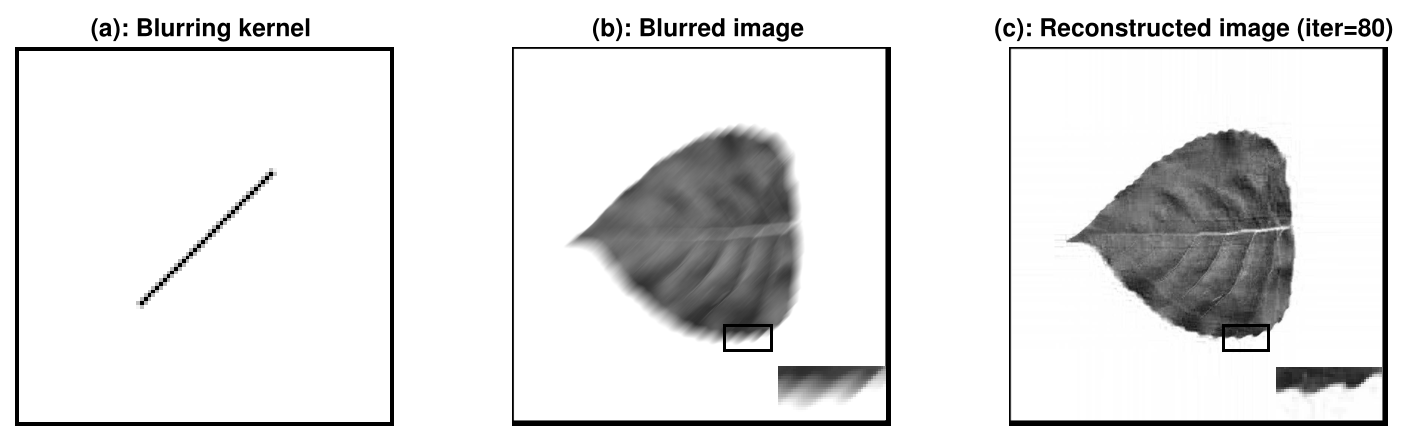
The motion kernel77 7 The blurring kernel is obtained by Matlab commands: “fspecial(’motion’, 50, 45)”. and the corresponding blurred image are shown in (a) and (b) of Figure 4. We assume that the support of the blurring kernel is known.
Refer to caption
Figure 4: Left: the blurring kernel; middle: the blurred image; right: the reconstructed image

The number of nonzero entries in the blurring kernel is K=109K=109. The most-significant wavelet subspaces with N=20000N=20000 are able to capture 97% of the energy in the original image. Algorithm 3 stops when the number of iterations is 20,40,60,80,100,120,14020,40,60,80,100,120,140, 160160, or 20002000. The reconstructed image using 80 iterations is given in (c) of Figure 4. As shown in Table 2, a higher accuracy does not improve the recovery performance in the sense that the relative error r​e​l​e​r​rrelerr, defined in Table 2, does not necessarily decrease as the number of iterations increases. In the later experiments, the number of iterations is set to be 80.

Table 2: The computational costs for multiple values of NN in Figure 4. n​B​hnBh, n​C​mnCm, and n​F​F​TnFFT are defined in Table 1. tt denotes the computational time in seconds. r​e​l​r​e​srelres denotes ‖y−diag⁡(Bhm∗​C∗)‖2/‖y‖2\|y-\diag(Bhm^{*}C^{*})\|_{2}/\|y\|_{2}. r​e​l​l​e​r​rrellerr denotes ‖𝐲^−‖𝐲‖‖𝐲f‖​𝐲f‖/‖𝐲^‖\left\|\mathbf{\hat{y}}-\frac{\|\mathbf{y}\|}{\|\mathbf{y}_{f}\|}\mathbf{y}_{f}\right\|/\|\mathbf{\hat{y}}\|, where 𝐲f\mathbf{y}_{f} denotes the vector obtained by reshaping a reconstructed image.
n​u​m.num. o​fof i​t​e​r.iter. 20 40 60 80 100 120 140 160 2000
r​e​l​r​e​srelres 3.9−33.9_{-3} 2.6−32.6_{-3} 2.5−32.5_{-3} 2.4−32.4_{-3} 2.3−32.3_{-3} 2.3−32.3_{-3} 2.2−32.2_{-3} 2.2−32.2_{-3} 2.0−32.0_{-3}
n​B​h/n​C​mnBh/nCm 43 85 125 168 210 253 294 335 4055
n​F​F​TnFFT 107 211 311 417 521 627 729 831 10111
r​e​l​e​r​rrelerr 4.1−24.1_{-2} 3.8−23.8_{-2} 3.8−23.8_{-2} 3.8−23.8_{-2} 4.1−24.1_{-2} 4.2−24.2_{-2} 4.3−24.3_{-2} 4.4−24.4_{-2} 6.4−26.4_{-2}

Other kernels with known supports:

Two blurring kernels, their corresponding blurred images, and the reconstructed images are shown in Figures 5 and 6. The blurring kernel in Figure 5 is from the function sin\sin and has 153 nonzero entries. The covariance of the Gaussian kernel in Figure 6 is V=[10.80.81]V=\begin{bmatrix}1&0.8\\ 0.8&1\end{bmatrix} and the number of nonzero entries is 181.

The number of iterations is 80 and their computational times are approximately 48 seconds. The relative errors r​e​l​e​r​rrelerr, defined in Table 2, of the “sin\sin” kernel and the Gaussian kernel are 0.03980.0398 and 0.08900.0890, respectively. We can see that the Riemannian method is able to recover a reasonable image for a more complex kernel.

Refer to caption
Figure 5: Left: the blurring kernel; middle: the blurred image; right: the reconstructed image
Refer to caption
Figure 6: Left: the blurring kernel; middle: the blurred image; right: the reconstructed image

Motion kernel with unknown support:

The motion kernel in (a) of Figure 4 is used. In practice, the true support of the kernel is unknown and an estimation is usually not exact. Figure 7 shows the recovery performance of the Riemannian method when an inexact support is used. We use four inexact supports, which are obtained by enlarging the true support by 1, 2, 3, and 4 pixels. Unsurprisingly, the better the estimation of the support is, the better the reconstructed image is. The Riemannian method is able to recover the image reasonably in these tests.

Refer to caption
Figure 7: Deconvolution results for unknown supports. Top: the estimated support of the blurring kernel. Bottom: the reconstructed images using the corresponding above supports. The relative error r​e​l​e​r​rrelerr from left to right are 0.04400.0440, 0.04840.0484, 0.05220.0522, and 0.06730.0673, respectively.

6 Conclusion

In this paper, we proposed a Riemannian steepest descent method for blind deconvolution. By inspiring the proofs in [LLSW16], it is proven that the Riemannian method with an appropriate initialization has high probability to successfully recover the desired signal. Since a quotient manifold is considered, the penalty term that is used to control the norm of hh and mm is not necessary. The Hessian at the desired solution is proven to be well-conditioned with high probability and therefore the optimization is not difficult locally. Numerical experiments show that the Riemannian steepest descent method is robust to noise, is the most efficient algorithm, and has the empirical largest successful recovery probability among the alternating minimization algorithm and the algorithm in [LLSW16].

References

  • [AMS08] P.-A. Absil, R. Mahony, and R. Sepulchre. Optimization algorithms on matrix manifolds. Princeton University Press, Princeton, NJ, 2008.
  • [ARR14] A. Ahmed, B. Recht, and J. Romberg. Blind deconvolution using convex programming. IEEE Transactions on Information Theory, 60(3):1711–1732, March 2014.
  • [BA11] N. Boumal and P.-A. Absil. RTRMC: A Riemannian trust-region method for low-rank matrix completion. Advances in Neural Information Processing Systems 24 (NIPS), pages 406–414, 2011.
  • [Bak08] C. G. Baker. Riemannian manifold trust-region methods with applications to eigenproblems. PhD thesis, Florida State University, Department of Computational Science, 2008.
  • [BB88] J. Barzilai and J. M. Borwein. Two-Point Step Size Gradient Methods. IMA Journal of Numerical Analysis, 8:141–148, 1988.
  • [BM03] S. Burer and R. D. C. Monteiro. A nonlinear programming algorithm for solving semidefinite programs via low-rank factorization. Mathematical Programming, 95(2):329–357, February 2003. doi:10.1007/s10107-002-0352-8.
  • [BSA13] N. Boumal, A. Singer, and P.-A. Absil. Robust estimation of rotations from relative measurements by maximum likelihood. 52nd IEEE Conference on Decision and Control, (3):1156–1161, December 2013. doi:10.1109/CDC.2013.6760038.
  • [CE07] P. Campisi and K. Egiazarian. Blind image deconvolution : theory and applications. CRC press, 2007.
  • [CLS16] E. J. Candés, X. Li, and M. Soltanolkotabi. Phase retrieval via Wirtinger flow: theory and algorithms. IEEE Transactions on Information Theory, 64(4):1985–2007, 2016.
  • [FJ05] Matteo Frigo and Steven G. Johnson. The design and implementation of FFTW3. Proceedings of the IEEE, 93(2):216–231, 2005. Special issue on “Program Generation, Optimization, and Platform Adaptation”.
  • [GV96] G. H. Golub and C. F. Van Loan. Matrix computations. Johns Hopkins Studies in the Mathematical Sciences. Johns Hopkins University Press, third edition, 1996.
  • [HAG15] W. Huang, P.-A. Absil, and K. A. Gallivan. A Riemannian symmetric rank-one trust-region method. Mathematical Programming, 150(2):179–216, February 2015.
  • [HAG16] W. Huang, P.-A. Absil, and K. A. Gallivan. Intrinsic representation of tangent vectors and vector transport on matrix manifolds. Numerische Mathematik, 136(2):523–543, 2016.
  • [HAG18] Wen Huang, P.-A. Absil, and K. A. Gallivan. A Riemannian BFGS Method without Differentiated Retraction for Nonconvex Optimization Problems. SIAM Journal on Optimization, 28(1):470–495, 2018.
  • [HAGH16] Wen Huang, P.-A. Absil, K. A. Gallivan, and Paul Hand. ROPTLIB: an object-oriented C++ library for optimization on Riemannian manifolds. Technical Report FSU16-14, Florida State University, 2016.
  • [HGA15] W. Huang, K. A. Gallivan, and P.-A. Absil. A Broyden Class of Quasi-Newton Methods for Riemannian Optimization. SIAM Journal on Optimization, 25(3):1660–1685, 2015.
  • [HGZ17] Wen Huang, K. A. Gallivan, and Xiangxiong Zhang. Solving PhaseLift by low rank Riemannian optimization methods for complex semidefinite constraints. SIAM Journal on Scientific Computing, 39(5):B840–B859, 2017.
  • [Hua13] W. Huang. Optimization algorithms on Riemannian manifolds with applications. PhD thesis, Florida State University, Department of Mathematics, 2013.
  • [JC93] S. M. Jefferies and J. C. Christou. Restoration of astronomical images by iterative blind deconvolution. The Astrophysical Journal, page 415:862, 1993.
  • [LLJB15] K. Lee, Y. Li, M. Junge, and Y. Bresler. Blind Recovery of Sparse Signals from Subsampled Convolution. pages 1–43, 2015.
  • [LLSW16] Xiaodong Li, Shuyang Ling, Thomas Strohmer, and Ke Wei. Rapid, robust, and reliable blind deconvolution via nonconvex optimization. CoRR, abs/1606.04933, 2016.
  • [LS15] S. Ling and T. Strohmer. Self-Calibration and Biconvex Compressive Sensing. Inverse Problems, 31(11):115002, 2015.
  • [LWDF11] A. Levin, Y. Weiss, F. Durand, and W. T. Freeman. Understanding and evaluating blind deconvolution algorithms. IEEE Transactions on Pattern Analysis and Machine Intelligence, 33(12):2354–2367, 2011.
  • [Mis14] B. Mishra. A Riemannian approach to large-scale constrained least-squares with symmetries. PhD thesis, University of Liege, 2014.
  • [NW06] J. Nocedal and S. J. Wright. Numerical Optimization. Springer, second edition, 2006.
  • [RW12] W. Ring and B. Wirth. Optimization methods on Riemannian manifolds and their application to shape space. SIAM Journal on Optimization, 22(2):596–627, January 2012. doi:10.1137/11082885X.
  • [Sat16] H. Sato. A Dai–Yuan-type Riemannian conjugate gradient method with the weak Wolfe conditions. Computational Optimization and Applications, 64(1):101–118, May 2016.
  • [SI15] H. Sato and T. Iwai. A new, globally convergent Riemannian conjugate gradient method. Optimization, 64(4):1011–1031, February 2015.
  • [SL16] Ruoyu Sun and Zhi Quan Luo. Guaranteed Matrix Completion via Non-Convex Factorization. IEEE Transactions on Information Theory, 62(11):6535–6579, 2016.
  • [Van13] B. Vandereycken. Low-rank matrix completion by Riemannian optimization—extended version. SIAM Journal on Optimization, 23(2):1214–1236, 2013.
  • [WBSJ15] G. Wunder, H. Boche, T. Strohmer, and P. Jung. Sparse Signal Processing Concepts for Efficient 5G System Design. IEEE Access, 3:195–208, 2015.
  • [WBX+07] S. G. Wu, F. S. Bao, E. Y. Xu, Y.-X. Wang, Y.-F. Chang, and Q.-L. Xiang. A leaf recognition algorithm for plant classification using probabilistic neural network. 2007 IEEE International Symposium on Signal Processing and Information Technology, pages 11–16, 2007. arXiv:0707.4289v1.
  • [WCCL16] K. Wei, J.-F. Cai, T. F. Chan, and S. Leung. Guarantees of Riemannian Optimization for Low Rank Matrix Completion. (1), 2016.
  • [WP98] X. Wang and H. V. Poor. Blind Equalization and Multiuser Detection in Dispersive CDMA Channels. IEEE Transactions on Communications, 46(1):91–103, 1998.
  • [YK94] T.-L. You and M. Kaveh. A simple algorithm for joint blur identification and image restoration. Proceedings - International Conference on Image Processing, ICIP, 3(3):167–171, 1994.
  • [Zhu17] X. Zhu. A Riemannian conjugate gradient method for optimization on the Stiefel manifold. Computational Optimization and Applications, 67(1):73–110, 2017.

Appendix A Four Conditions and the Proof of Theorem 3.2

The convergence analysis of the Riemannian steepest descent method follows the spirit of the analysis in [LLSW16] and the analyses both rely on the four conditions: local RIP condition, robustness condition, local regularity condition and local smoothness condition. There exist differences and the main ones are highlighted as follows. The differences ease the proofs of the Riemannian method in general.

  • •

    The cost function f~\tilde{f} does not include the penalty terms for the norm of hh and mm. Therefore, the penalty terms are not considered in the convergence analysis.

  • •

    Since any representation in π−1​(π​(h,m))\pi^{-1}(\pi(h,m)) can be used and this does not influence the sequence {π⁡(hk,mk)}\{\pi(h_{k},m_{k})\} of 𝒬1\mathcal{Q}_{1} generated by Algorithm 4, we can always assume ‖hk‖2=‖mk‖2\|h_{k}\|_{2}=\|m_{k}\|_{2} without loss of generality.

  • •

    The Riemannian gradient is different from the Wirtinger derivative. For the cost function FF in (1.4), if ‖h‖2=‖m‖2\|h\|_{2}=\|m\|_{2}, then by (4.9) and (3.4), we have

    grad⁡F⁡(h,m)=2‖hm∗‖2​∇wF​(h,m).\grad F(h,m)=\frac{2}{\|hm^{*}\|_{2}}\nabla^{w}F(h,m).

Let π⁡(h♯,m♯)\pi(h_{\sharp},m_{\sharp}) denote the ground truth and Υf~\Upsilon_{\tilde{f}} denote {π⁡(h,m)∣f~​(π⁡(h,m))≤13​ε2​d∗2+‖e‖22}\{\pi(h,m)\mid\tilde{f}(\pi(h,m))\leq\frac{1}{3}\varepsilon^{2}d_{*}^{2}+\|e\|_{2}^{2}\}.

Condition A.1 (Local RIP condition).

The following local Restricted Isometry Property for 𝒜\mathcal{A} holds uniformly for all (h,m)∈Πε(h,m)\in\Pi_{\varepsilon}:

34​‖h​m∗−h♯​m♯∗‖F2≤‖𝒜⁡(h​m∗−h♯​m♯∗)‖22≤54​‖h​m∗−h♯​m♯∗‖F2.\frac{3}{4}\|hm^{*}-h_{\sharp}m_{\sharp}^{*}\|_{F}^{2}\leq\|\mathcal{A}(hm^{*}-h_{\sharp}m_{\sharp}^{*})\|_{2}^{2}\leq\frac{5}{4}\|hm^{*}-h_{\sharp}m_{\sharp}^{*}\|_{F}^{2}.
Condition A.2 (Robustness condition).

If L≥Cγ​(σ2/ε2+σ/ε)​max⁡(K,N)​log⁡(L)L\geq C_{\gamma}(\sigma^{2}/\varepsilon^{2}+\sigma/\varepsilon)\max(K,N)\log(L), then with high probability, it holds that

‖𝒜∗​(e)‖2≤ε​d∗10​2.\|\mathcal{A}^{*}(e)\|_{2}\leq\frac{\varepsilon d_{*}}{10\sqrt{2}}.
Condition A.3 (Local regularity condition).

There exists a regularity constant a0>0a_{0}>0 such that

‖grad⁡f~​(π⁡(h,m))‖gπ⁡(h,m)2≥a0​[f~​(π⁡(h,m))−c]+\|\grad\tilde{f}(\pi(h,m))\|_{g_{\pi(h,m)}}^{2}\geq a_{0}[\tilde{f}(\pi(h,m))-c]_{+}

for all π⁡(h,m)∈Ωμ∩Πε\pi(h,m)\in\Omega_{\mu}\cap\Pi_{\varepsilon}, where c=‖e‖22+1700​‖𝒜∗​(e)‖22c=\|e\|_{2}^{2}+1700\|\mathcal{A}^{*}(e)\|_{2}^{2} and a0=1/1500a_{0}=1/1500.

Condition A.4 (Local smoothness condition).

Define the lifting function f^π⁡(h,m):Tπ⁡(h,m)⁡𝒬1→ℝ:ηπ⁡(h,m)=f~∘R~π⁡(h,m)​(ηπ⁡(h,m))\hat{f}_{\pi(h,m)}:\T_{\pi(h,m)}\mathcal{Q}_{1}\rightarrow\mathbb{R}:\eta_{\pi(h,m)}=\tilde{f}\circ\tilde{R}_{\pi(h,m)}(\eta_{\pi(h,m)}). There exists a constant aLa_{L} such that

‖grad⁡f^π⁡(h,m)​(t​ηπ⁡(h,m))−grad⁡f^π⁡(h,m)​(0)‖g(h,m)≤aL​t​‖ηπ⁡(h,m)‖g(h,m),∀0≤t≤1,\|\grad\hat{f}_{\pi(h,m)}(t\eta_{\pi(h,m)})-\grad\hat{f}_{\pi(h,m)}(0)\|_{g_{(h,m)}}\leq a_{L}t\|\eta_{\pi(h,m)}\|_{g_{(h,m)}},\;\;\;\forall 0\leq t\leq 1,

for all π⁡(h,m)\pi(h,m) and ηπ⁡(h,m)∈Tπ⁡(h,m)⁡𝒬1\eta_{\pi(h,m)}\in\T_{\pi(h,m)}\mathcal{Q}_{1} such that R~π⁡(h,m)​(t​ηπ⁡(h,m))∈Υf~∩Πε,∀0≤t≤1\tilde{R}_{\pi(h,m)}(t\eta_{\pi(h,m)})\in\Upsilon_{\tilde{f}}\cap\Pi_{\varepsilon},\forall 0\leq t\leq 1, where R~\tilde{R} is defined in (4.5).

Conditions A.1 and A.2 are the same as [LLSW16, Conditions 5.1 and 5.2] and have been proven therein. Conditions A.3 and A.4 are different from[LLSW16, Conditions 5.3 and 5.4] since we use different penalty term and different gradient and norm. The proofs of Conditions A.3 and A.4 are given in Section B.

Lemma A.1 generalizes [LLSW16, Lemma 6.1] and is used in Lemma A.2.

Lemma A.1 (Riemannian descent lemma).

Suppose Condition A.4 holds. Then

f^π⁡(h,m)​(ηπ⁡(h,m))≤f^​(0π⁡(h,m))+gπ⁡(h,m)​(ηπ⁡(h,m),grad⁡f~​(π⁡(h,m)))+aL​‖ηπ⁡(h,m)‖g2,\hat{f}_{\pi(h,m)}(\eta_{\pi(h,m)})\leq\hat{f}(0_{\pi(h,m)})+g_{\pi(h,m)}(\eta_{\pi(h,m)},\grad\tilde{f}(\pi(h,m)))+a_{L}\|\eta_{\pi(h,m)}\|_{g}^{2},

where 0π⁡(h,m)0_{\pi(h,m)} denotes the origin of Tπ⁡(h,m)⁡𝒬1\T_{\pi(h,m)}\mathcal{Q}_{1}.

Proof.

Define β⁡(t)=f^π⁡(h,m)​(t​ηπ⁡(h,m))\beta(t)=\hat{f}_{\pi(h,m)}(t\eta_{\pi(h,m)}). We have dd​t​β​(t)=g⁡(grad⁡f^π⁡(h,m)​(t​ηπ⁡(h,m)),ηπ⁡(h,m)).\frac{d}{dt}\beta(t)=g\left(\grad\hat{f}_{\pi(h,m)}(t\eta_{\pi(h,m)}),\eta_{\pi(h,m)}\right). It follows from the Fundamental Theorem of Calculus that

f^π⁡(h,m)\displaystyle\hat{f}_{\pi(h,m)} (ηπ⁡(h,m))−f^​(0)=∫01dd​t​β​(t)​𝑑t=∫01g⁡(grad⁡f^π⁡(h,m)​(t​ηπ⁡(h,m)),ηπ⁡(h,m))​𝑑t\displaystyle(\eta_{\pi(h,m)})-\hat{f}(0)=\int_{0}^{1}\frac{d}{dt}\beta(t)dt=\int_{0}^{1}g\left(\grad\hat{f}_{\pi(h,m)}(t\eta_{\pi(h,m)}),\eta_{\pi(h,m)}\right)dt
=\displaystyle= g⁡(grad⁡f^π⁡(h,m)​(0π⁡(h,m)),ηπ⁡(h,m))+∫01g⁡(grad⁡f^π⁡(h,m)​(t​ηπ⁡(h,m))−grad⁡f^π⁡(h,m)​(0π⁡(h,m)),ηπ⁡(h,m))​𝑑t\displaystyle g\left(\grad\hat{f}_{\pi(h,m)}(0_{\pi(h,m)}),\eta_{\pi(h,m)}\right)+\int_{0}^{1}g\left(\grad\hat{f}_{\pi(h,m)}(t\eta_{\pi(h,m)})-\grad\hat{f}_{\pi(h,m)}(0_{\pi(h,m)}),\eta_{\pi(h,m)}\right)dt
≤\displaystyle\leq g⁡(grad⁡f^π⁡(h,m)​(0π⁡(h,m)),ηπ⁡(h,m))+aL​‖ηπ⁡(h,m)‖g2.\displaystyle g\left(\grad\hat{f}_{\pi(h,m)}(0_{\pi(h,m)}),\eta_{\pi(h,m)}\right)+a_{L}\|\eta_{\pi(h,m)}\|_{g}^{2}.

Therefore, the result holds since grad⁡f^π⁡(h,m)​(0π⁡(h,m))=grad⁡f~​(π⁡(h,m))\grad\hat{f}_{\pi(h,m)}(0_{\pi(h,m)})=\grad\tilde{f}(\pi(h,m)), see [AMS08, (4.4)]. ∎

Lemma A.2 is used in the proof of Theorem 3.2. Note that this lemma follows from [LLSW16, Section 5.1].

Lemma A.2.

The following properties hold under some of the four conditions.

  1. 1.

    Under conditions A.1 and A.2, function ff in (1.5) satisfies

    ‖e‖22+34​Δ2−ε​Δ​d∗5≤f⁡(π⁡(h,m))≤‖e‖22+54​Δ2+ε​Δ​d∗5\|e\|_{2}^{2}+\frac{3}{4}\Delta^{2}-\frac{\varepsilon\Delta d_{*}}{5}\leq f(\pi(h,m))\leq\|e\|_{2}^{2}+\frac{5}{4}\Delta^{2}+\frac{\varepsilon\Delta d_{*}}{5} (A.1)

    for all π⁡(h,m)∈Ωμ∩Πε\pi(h,m)\in\Omega_{\mu}\cap\Pi_{\varepsilon}, where Δ=‖h​m∗−h♯​m♯∗‖F\Delta=\|hm^{*}-h_{\sharp}m_{\sharp}^{*}\|_{F}.

  2. 2.

    It holds that Υf~⊂Ωμ\Upsilon_{\tilde{f}}\subset\Omega_{\mu}; under conditions A.1 and A.2, we have Υf~∩Πε⊂Π910​ε\Upsilon_{\tilde{f}}\cap\Pi_{\varepsilon}\subset\Pi_{\frac{9}{10}\varepsilon}.

  3. 3.

    Under conditions A.1 and A.2, if π⁡(h1,m1)∈Πε\pi(h_{1},m_{1})\in\Pi_{\varepsilon} and π⁡((1−λ)​h1+λ​h2,(1−λ)​m1+λ​m2)∈Υf~\pi\left((1-\lambda)h_{1}+\lambda h_{2},(1-\lambda)m_{1}+\lambda m_{2}\right)\in\Upsilon_{\tilde{f}} for all λ∈[0,1]\lambda\in[0,1], then π⁡(h2,m2)∈Πε\pi(h_{2},m_{2})\in\Pi_{\varepsilon}.

  4. 4.

    Under conditions A.1, A.2 and A.4, suppose the step size α≤12​aL\alpha\leq\frac{1}{2a_{L}}, where aLa_{L} is defined in Condition A.4 and π⁡(hk,mk)∈Πε∩Υf~\pi(h_{k},m_{k})\in\Pi_{\varepsilon}\cap\Upsilon_{\tilde{f}}, then it holds that π⁡(hk+1,mk+1)∈Πε∩Υf~\pi(h_{k+1},m_{k+1})\in\Pi_{\varepsilon}\cap\Upsilon_{\tilde{f}} and

    f~​(π⁡(hk+1,mk+1))≤f~​(π⁡(hk,mk))−α2​‖grad⁡f~​(π⁡(hk,mk))‖g2.\tilde{f}(\pi(h_{k+1},m_{k+1}))\leq\tilde{f}(\pi(h_{k},m_{k}))-\frac{\alpha}{2}\|\grad\tilde{f}(\pi(h_{k},m_{k}))\|_{g}^{2}.
Proof.

(1): This has been proven in [LLSW16, (5.5), (5.6)].

(2): If π⁡(h,m)∉Ωμ\pi(h,m)\notin\Omega_{\mu}, then G⁡(π⁡(h,m))≥ρ​G0​(2​d∗2d2)G(\pi(h,m))\geq\rho G_{0}(\frac{2d_{*}^{2}}{d^{2}}). It follows that

f~​(π​(h,m))≥\displaystyle\tilde{f}(\pi(h,m))\geq ρ​G0​(2​d∗2d2)≥(d2+2.5​‖e‖22)​(2​d∗2d2−1)2\displaystyle\rho G_{0}(\frac{2d_{*}^{2}}{d^{2}})\geq(d^{2}+2.5\|e\|_{2}^{2})\left(\frac{2d_{*}^{2}}{d^{2}}-1\right)^{2}
≥\displaystyle\geq d2​(2​d∗2d2−1)2+2.5​‖e‖22​(2​d∗2d2−1)2≥13​ε2​d∗2+‖e‖22,\displaystyle d^{2}\left(\frac{2d_{*}^{2}}{d^{2}}-1\right)^{2}+2.5\|e\|_{2}^{2}\left(\frac{2d_{*}^{2}}{d^{2}}-1\right)^{2}\geq\frac{1}{3}\varepsilon^{2}d_{*}^{2}+\|e\|_{2}^{2},

where ρ≥d2+2.5​‖e‖22\rho\geq d^{2}+2.5\|e\|_{2}^{2}, ε<1/15\varepsilon<1/15, and 0.9​d∗≤d≤1.1​d∗0.9d_{*}\leq d\leq 1.1d_{*}. Therefore, π⁡(h,m)∉Υf~\pi(h,m)\notin\Upsilon_{\tilde{f}} and Υf~⊂Ωμ\Upsilon_{\tilde{f}}\subset\Omega_{\mu}.

For any π⁡(h,m)∈Υf~∩Πε\pi(h,m)\in\Upsilon_{\tilde{f}}\cap\Pi_{\varepsilon}, it holds that π⁡(h,m)∈Ωμ∩Πε\pi(h,m)\in\Omega_{\mu}\cap\Pi_{\varepsilon}. It follows from (A.1) that ‖e‖22+34​Δ2−ε​Δ​d∗5≤f⁡(π⁡(h,m))≤f~​(π⁡(h,m))≤13​ε2​d∗2+‖e‖22\|e\|_{2}^{2}+\frac{3}{4}\Delta^{2}-\frac{\varepsilon\Delta d_{*}}{5}\leq f(\pi(h,m))\leq\tilde{f}(\pi(h,m))\leq\frac{1}{3}\varepsilon^{2}d_{*}^{2}+\|e\|_{2}^{2}, which can be simplified into 45​Δ2−12​ε​d∗​Δ−20​ε2​d∗2≤045\Delta^{2}-12\varepsilon d_{*}\Delta-20\varepsilon^{2}d_{*}^{2}\leq 0. This implies Δ≤0.9​ε​d∗\Delta\leq 0.9\varepsilon d_{*} and hence Υf~∩Πε⊂Π910​ε\Upsilon_{\tilde{f}}\cap\Pi_{\varepsilon}\subset\Pi_{\frac{9}{10}\varepsilon}.

(3): Prove by contradiction. If π⁡(h2,m2)∉Πε\pi(h_{2},m_{2})\notin\Pi_{\varepsilon}, then there exists λ0\lambda_{0} such that

‖((1−λ)​h1+λ​h2)​((1−λ)​m1+λ​m2)∗−h1​m1∗‖=ε​d∗,\|\left((1-\lambda)h_{1}+\lambda h_{2}\right)\left((1-\lambda)m_{1}+\lambda m_{2}\right)^{*}-h_{1}m_{1}^{*}\|=\varepsilon d_{*},

i.e., π⁡((1−λ)​h1+λ​h2,(1−λ)​m1+λ​m2)∈∂Πε\pi\left((1-\lambda)h_{1}+\lambda h_{2},(1-\lambda)m_{1}+\lambda m_{2}\right)\in\partial\Pi_{\varepsilon}. Therefore, it follows from

π⁡((1−λ)​h1+λ​h2,(1−λ)​m1+λ​m2)∈Υf~\pi\left((1-\lambda)h_{1}+\lambda h_{2},(1-\lambda)m_{1}+\lambda m_{2}\right)\in\Upsilon_{\tilde{f}}

that π⁡((1−λ)​h1+λ​h2,(1−λ)​m1+λ​m2)∈Π0.9​ε\pi\left((1-\lambda)h_{1}+\lambda h_{2},(1-\lambda)m_{1}+\lambda m_{2}\right)\in\Pi_{0.9\varepsilon}. This is a contradiction.

(4): If grad⁡f~​(π⁡(hk,mk))=0\grad\tilde{f}(\pi(h_{k},m_{k}))=0, then π⁡(hk+1,mk+1)=π⁡(hk,mk)∈Πε∩Υf~\pi(h_{k+1},m_{k+1})=\pi(h_{k},m_{k})\in\Pi_{\varepsilon}\cap\Upsilon_{\tilde{f}}. Suppose grad⁡f~​(π⁡(hk,mk))≠0\grad\tilde{f}(\pi(h_{k},m_{k}))\neq 0. Define the function

ϕ⁡(λ)=f^π⁡(hk,mk)​(−λ​grad⁡f~​(π⁡(hk,mk))).\phi(\lambda)=\hat{f}_{\pi(h_{k},m_{k})}(-\lambda\grad\tilde{f}(\pi(h_{k},m_{k}))).

It follows that ϕ′​(0)=−‖grad⁡f~​(π⁡(hk,mk))‖g2<0\phi^{\prime}(0)=-\|\grad\tilde{f}(\pi(h_{k},m_{k}))\|_{g}^{2}<0. By Lemma A.1, we have

ϕ⁡(λ)≤\displaystyle\phi(\lambda)\leq ϕ⁡(0)−λ​‖grad⁡f~​(π⁡(hk,mk))‖g2+aL​λ2​‖grad⁡f~​(π⁡(hk,mk))‖g2\displaystyle\phi(0)-\lambda\|\grad\tilde{f}(\pi(h_{k},m_{k}))\|_{g}^{2}+a_{L}\lambda^{2}\|\grad\tilde{f}(\pi(h_{k},m_{k}))\|_{g}^{2} (A.2)
=\displaystyle= ϕ⁡(0)+(aL​λ2−λ)​‖grad⁡f~​(π⁡(hk,mk))‖g2≤ϕ⁡(0)\displaystyle\phi(0)+(a_{L}\lambda^{2}-\lambda)\|\grad\tilde{f}(\pi(h_{k},m_{k}))\|_{g}^{2}\leq\phi(0) (A.3)

for all λ∈[0,α]\lambda\in[0,\alpha]. Therefore, by (3) in Lemma A.2, we have π⁡(hk+1,mk+1)∈Πε∩Υf~\pi(h_{k+1},m_{k+1})\in\Pi_{\varepsilon}\cap\Upsilon_{\tilde{f}}. Using (A.3) yields

f~​(π⁡(hk+1,mk+1))≤f~​(π⁡(hk,mk))−α2​‖grad⁡f~​(π⁡(hk,mk))‖g2.\tilde{f}(\pi(h_{k+1},m_{k+1}))\leq\tilde{f}(\pi(h_{k},m_{k}))-\frac{\alpha}{2}\|\grad\tilde{f}(\pi(h_{k},m_{k}))\|_{g}^{2}.

∎

Now, we are ready to prove Theorem 3.2. With the four conditions, the proof follows from the proof in [LLSW16] and we give here for completeness.

Proof.

Since π⁡(h0,m0)∈Ω12​μ∩Π25​ε\pi(h_{0},m_{0})\in\Omega_{\frac{1}{2}\mu}\cap\Pi_{\frac{2}{5}\varepsilon}, we have

L​|bi∗​h0|2​‖m0‖228​d2​μ2≤L8​d2​μ2​4​d∗2​μ2L≤d∗22​d2<1,\frac{L|b_{i}^{*}h_{0}|^{2}\|m_{0}\|_{2}^{2}}{8d^{2}\mu^{2}}\leq\frac{L}{8d^{2}\mu^{2}}\frac{4d_{*}^{2}\mu^{2}}{L}\leq\frac{d_{*}^{2}}{2d^{2}}<1,

where L​‖B​h0‖∞​‖m‖2≤2​d∗​μ\sqrt{L}\|Bh_{0}\|_{\infty}\|m\|_{2}\leq 2d_{*}\mu. Therefore, the penalty term G⁡(π⁡(h0,m0))=0G(\pi(h_{0},m_{0}))=0. Combining (A.1) and Δ≤25​ε​d∗\Delta\leq\frac{2}{5}\varepsilon d_{*} yields

f~​(π⁡(h,m))=f⁡(π⁡(h,m))≤‖e‖22+54​Δ2+ε​Δ​d∗5≤13​ε2​d∗2+‖e‖22,\tilde{f}(\pi(h,m))=f(\pi(h,m))\leq\|e\|_{2}^{2}+\frac{5}{4}\Delta^{2}+\frac{\varepsilon\Delta d_{*}}{5}\leq\frac{1}{3}\varepsilon^{2}d_{*}^{2}+\|e\|_{2}^{2},

which implies π⁡(h0,m0)∈Υf~\pi(h_{0},m_{0})\in\Upsilon_{\tilde{f}}. It follows from (4) in Lemma A.2 and Condition A.3 that

f~​(π⁡(hk+1,mk+1))≤f~​(π⁡(hk,mk))−α​a02​[f~​(π⁡(hk,mk))−c]+\tilde{f}(\pi(h_{k+1},m_{k+1}))\leq\tilde{f}(\pi(h_{k},m_{k}))-\frac{\alpha a_{0}}{2}\left[\tilde{f}(\pi(h_{k},m_{k}))-c\right]_{+}

and π⁡(hk,mk)∈Ωμ∩Πε\pi(h_{k},m_{k})\in\Omega_{\mu}\cap\Pi_{\varepsilon} for all kk. Therefore, we have

f~​(π⁡(hk+1,mk+1))−c≤(1−α​a02)​[f~​(π⁡(hk,mk))−c]+\tilde{f}(\pi(h_{k+1},m_{k+1}))-c\leq\left(1-\frac{\alpha a_{0}}{2}\right)\left[\tilde{f}(\pi(h_{k},m_{k}))-c\right]_{+}

which implies

[f~​(π⁡(hk+1,mk+1))−c]+≤(1−α​a02)​[f~​(π⁡(hk,mk))−c]+.\left[\tilde{f}(\pi(h_{k+1},m_{k+1}))-c\right]_{+}\leq\left(1-\frac{\alpha a_{0}}{2}\right)\left[\tilde{f}(\pi(h_{k},m_{k}))-c\right]_{+}.

Thus, we obtain

[f~​(π⁡(hk,mk))−c]+≤(1−α​a02)k​[f~​(π⁡(h0,m0))−c]+≤13​(1−α​a02)k​ε2​d∗2,\left[\tilde{f}(\pi(h_{k},m_{k}))-c\right]_{+}\leq\left(1-\frac{\alpha a_{0}}{2}\right)^{k}\left[\tilde{f}(\pi(h_{0},m_{0}))-c\right]_{+}\leq\frac{1}{3}\left(1-\frac{\alpha a_{0}}{2}\right)^{k}\varepsilon^{2}d_{*}^{2},

where we use f~​(π⁡(h0,m0))≤13​ε2​d∗2+‖e‖22\tilde{f}(\pi(h_{0},m_{0}))\leq\frac{1}{3}\varepsilon^{2}d_{*}^{2}+\|e\|_{2}^{2} and c=‖e‖22+1700​‖𝒜∗​(e)‖22≥‖e‖22c=\|e\|_{2}^{2}+1700\|\mathcal{A}^{*}(e)\|_{2}^{2}\geq\|e\|_{2}^{2}. We also have

f~​(π⁡(hk,mk))−‖e‖22≥\displaystyle\tilde{f}(\pi(h_{k},m_{k}))-\|e\|_{2}^{2}\geq ‖𝒜⁡(hk​mk∗−h♯​m♯∗)‖22−2​R​e​(⟨𝒜∗​(e),hk​mk∗−h♯​m♯∗⟩2)\displaystyle\|\mathcal{A}(h_{k}m_{k}^{*}-h_{\sharp}m_{\sharp}^{*})\|_{2}^{2}-2\mathrm{Re}({\left\langle\mathcal{A}^{*}(e),h_{k}m_{k}^{*}-h_{\sharp}m_{\sharp}^{*}\right\rangle_{2}})
≥\displaystyle\geq 34​‖hk​mk∗−h♯​m♯∗‖F2−2​2​‖𝒜∗​(e)‖2​‖hk​mk∗−h♯​m♯∗‖F.\displaystyle\frac{3}{4}\|h_{k}m_{k}^{*}-h_{\sharp}m_{\sharp}^{*}\|_{F}^{2}-2\sqrt{2}\|\mathcal{A}^{*}(e)\|_{2}\|h_{k}m_{k}^{*}-h_{\sharp}m_{\sharp}^{*}\|_{F}.

It follows that

13​(1−α​a02)k​ε2​d∗2≥[f~​(π⁡(hk,mk))−c]+≥34​‖hk​mk∗−h♯​m♯∗‖F2−2​2​‖𝒜∗​(e)‖2​‖hk​mk∗−h♯​m♯∗‖F−1700​‖𝒜∗​(e)‖22,\frac{1}{3}\left(1-\frac{\alpha a_{0}}{2}\right)^{k}\varepsilon^{2}d_{*}^{2}\geq\left[\tilde{f}(\pi(h_{k},m_{k}))-c\right]_{+}\geq\frac{3}{4}\|h_{k}m_{k}^{*}-h_{\sharp}m_{\sharp}^{*}\|_{F}^{2}-2\sqrt{2}\|\mathcal{A}^{*}(e)\|_{2}\|h_{k}m_{k}^{*}-h_{\sharp}m_{\sharp}^{*}\|_{F}-1700\|\mathcal{A}^{*}(e)\|_{2}^{2},

which is equivalent to

|‖hk​mk∗−h♯​m♯∗‖F−4​23​‖𝒜∗​(e)‖2|2≤49​(1−α​a02)t​ε2​d∗2+(68003+329)​‖𝒜∗​(e)‖22.\left|\|h_{k}m_{k}^{*}-h_{\sharp}m_{\sharp}^{*}\|_{F}-\frac{4\sqrt{2}}{3}\|\mathcal{A}^{*}(e)\|_{2}\right|^{2}\leq\frac{4}{9}\left(1-\frac{\alpha a_{0}}{2}\right)^{t}\varepsilon^{2}d_{*}^{2}+(\frac{6800}{3}+\frac{32}{9})\|\mathcal{A}^{*}(e)\|_{2}^{2}.

Solving for ‖hk​mkT−h♯​m♯T‖F\|h_{k}m_{k}^{T}-h_{\sharp}m_{\sharp}^{T}\|_{F} yields

‖hk​mkT−h♯​m♯T‖F≤23​(1−α​a02)k/2​ε​d∗+50​‖𝒜∗​(e)‖2.\|h_{k}m_{k}^{T}-h_{\sharp}m_{\sharp}^{T}\|_{F}\leq\frac{2}{3}\left(1-\frac{\alpha a_{0}}{2}\right)^{k/2}\varepsilon d_{*}+50\|\mathcal{A}^{*}(e)\|_{2}.

The upper bound for ‖𝒜∗​(e)‖2\|\mathcal{A}^{*}(e)\|_{2} has been proven in [LLSW16]. ∎

Appendix B Proofs of Conditions A.3 and A.4 and Theorem 3.1

Define function f~T=f~∘π\tilde{f}_{\mathrm{T}}=\tilde{f}\circ\pi, fT=f∘πf_{\mathrm{T}}=f\circ\pi, and GT=G∘πG_{\mathrm{T}}=G\circ\pi, which is defined in the total space ℝ∗K×ℝ∗N\mathbb{R}_{*}^{K}\times\mathbb{R}_{*}^{N}. Since the function value fT​(h,m)f_{\mathrm{T}}(h,m) and ‖grad⁡fT​(h,m)‖g\|\grad f_{\mathrm{T}}(h,m)\|_{g} are independent of representation in π−1​(π​(h,m))\pi^{-1}(\pi(h,m)), we can always choose hh and mm such that ‖h‖2=‖m‖2\|h\|_{2}=\|m\|_{2}. For all π⁡(h,m)∈Πε\pi(h,m)\in\Pi_{\varepsilon}, we have ‖h‖2​‖m‖2=‖h​m∗‖F≤‖h​m∗−h♯​m♯∗‖F+‖h♯​m♯∗‖F≤(1+ε)​d∗\|h\|_{2}\|m\|_{2}=\|hm^{*}\|_{F}\leq\|hm^{*}-h_{\sharp}m_{\sharp}^{*}\|_{F}+\|h_{\sharp}m_{\sharp}^{*}\|_{F}\leq(1+\varepsilon)d_{*} and ‖h‖2​‖m‖2=‖h​m∗‖F≥‖h♯​m♯∗‖F−‖h​m∗−h♯​m♯∗‖F≥(1−ε)​d∗\|h\|_{2}\|m\|_{2}=\|hm^{*}\|_{F}\geq\|h_{\sharp}m_{\sharp}^{*}\|_{F}-\|hm^{*}-h_{\sharp}m_{\sharp}^{*}\|_{F}\geq(1-\varepsilon)d_{*}. It follows that

(h,m)∈Ωd:={(h,m)∣1415​d∗≤‖h‖2=‖m‖2≤1615​d∗},(h,m)\in\Omega_{d}:=\left\{(h,m)\mid\sqrt{\frac{14}{15}d_{*}}\leq\|h\|_{2}=\|m\|_{2}\leq\sqrt{\frac{16}{15}d_{*}}\right\}, (B.1)

for all π⁡(h,m)∈Πε\pi(h,m)\in\Pi_{\varepsilon} and ε≤1/15\varepsilon\leq 1/15. There are unique orthogonal decompositions

h=τ1​h♯+h~​ and ​m=τ2​m♯+m~,h=\tau_{1}h_{\sharp}+\tilde{h}\hbox{ and }m=\tau_{2}m_{\sharp}+\tilde{m},

where h~∗​h♯=0\tilde{h}^{*}h_{\sharp}=0 and m~∗​m♯=0\tilde{m}^{*}m_{\sharp}=0. Let

h^=h−τ​h♯​ and ​m^=m−τ¯−1​m♯,\hat{h}=h-\tau h_{\sharp}\hbox{ and }\hat{m}=m-\bar{\tau}^{-1}m_{\sharp},

where τ=1(1−Δ10​d∗)​τ¯2\tau=\frac{1}{(1-\frac{\Delta}{10d_{*}})\bar{\tau}_{2}}.

Lemma B.1.

For all (h,m)(h,m) such that (h,m)∈Ωd(h,m)\in\Omega_{d} and π⁡(h,m)∈Πε\pi(h,m)\in\Pi_{\varepsilon} with ε≤1/15\varepsilon\leq 1/15, it holds that ‖h^‖22≤6.1​Δ2/d∗\|\hat{h}\|_{2}^{2}\leq 6.1\Delta^{2}/d_{*}, ‖m^‖22≤6.1​Δ2/d∗\|\hat{m}\|_{2}^{2}\leq 6.1\Delta^{2}/d_{*}, and ‖h^‖22​‖m^‖22≤8.4​Δ4/d∗2\|\hat{h}\|_{2}^{2}\|\hat{m}\|_{2}^{2}\leq 8.4\Delta^{4}/d_{*}^{2}. Moreover, if we assume π⁡(h,m)∈Ωμ\pi(h,m)\in\Omega_{\mu} additionally, we have L​‖B⁡(h^)‖∞≤6​μ​d∗\sqrt{L}\|B(\hat{h})\|_{\infty}\leq 6\mu\sqrt{d_{*}}.

Proof.

Inequalities ‖h^‖22≤6.1​Δ2/d∗\|\hat{h}\|_{2}^{2}\leq 6.1\Delta^{2}/d_{*}, ‖m^‖22≤6.1​Δ2/d∗\|\hat{m}\|_{2}^{2}\leq 6.1\Delta^{2}/d_{*}, and ‖h^‖22​‖m^‖22≤8.4​Δ4/d∗2\|\hat{h}\|_{2}^{2}\|\hat{m}\|_{2}^{2}\leq 8.4\Delta^{4}/d_{*}^{2} have been proven in [LLSW16, Lemma 5.15]. Note the definition of Ωμ\Omega_{\mu} and (B.1), we have {(h,m)∣L∥Bh∥∞∥m∥2≤4d∗μ,∥h∥2=∥m∥2}⊂{(h,m)∣L∥Bh∥∞≤4.5d∗μ}\{(h,m)\mid\sqrt{L}\|Bh\|_{\infty}\|m\|_{2}\leq 4d_{*}\mu,\|h\|_{2}=\|m\|_{2}\}\subset\{(h,m)\mid\sqrt{L}\|Bh\|_{\infty}\leq 4.5\sqrt{d_{*}}\mu\}. We also have |τ1​τ2¯|≥1−ε|\tau_{1}\bar{\tau_{2}}|\geq 1-\varepsilon by [LLSW16, Lemma 5.9] and |τ1|≤‖h‖2‖h♯‖2=‖h‖2​‖m‖2‖h♯‖2​‖m♯‖2≤‖h​m∗−h♯​m♯∗‖F+‖h♯​m♯∗‖Fd∗≤1+ε|\tau_{1}|\leq\frac{\|h\|_{2}}{\|h_{\sharp}\|_{2}}=\sqrt{\frac{\|h\|_{2}\|m\|_{2}}{\|h_{\sharp}\|_{2}\|m_{\sharp}\|_{2}}}\leq\sqrt{\frac{\|hm^{*}-h_{\sharp}m_{\sharp}^{*}\|_{F}+\|h_{\sharp}m_{\sharp}^{*}\|_{F}}{d_{*}}}\leq\sqrt{1+\varepsilon}. Therefore, it holds that

L​‖B⁡(h^)‖∞≤\displaystyle\sqrt{L}\|B(\hat{h})\|_{\infty}\leq L​‖B⁡(h)‖∞+1(1−Δ10​d∗)​τ¯2​L​‖B⁡(h♯)‖∞\displaystyle\sqrt{L}\|B(h)\|_{\infty}+\frac{1}{(1-\frac{\Delta}{10d_{*}})\bar{\tau}_{2}}\sqrt{L}\|B(h_{\sharp})\|_{\infty}
=\displaystyle= 4.5​μ​d∗+1+ε(1−Δ10​d∗)​(1−ε)≤5.7​μ​d∗,\displaystyle 4.5\mu\sqrt{d_{*}}+\frac{\sqrt{1+\varepsilon}}{(1-\frac{\Delta}{10d_{*}})(1-\varepsilon)}\leq 5.7\mu\sqrt{d_{*}},

where Δ/d∗≤ε≤1/15\Delta/d_{*}\leq\varepsilon\leq 1/15. ∎

Lemma 2.3 is the [LLSW16, Lemm 5.16] and is used in the proof of Condition A.3.

Lemma B.2.

For all (h,m)(h,m) such that (h,m)∈Ωd(h,m)\in\Omega_{d} and π⁡(h,m)∈Πε∩Ωμ\pi(h,m)\in\Pi_{\varepsilon}\cap\Omega_{\mu} with ε≤1/15\varepsilon\leq 1/15, it uniformly holds that

Re⁡(⟨∇hwfT,h^⟩2+⟨∇mwfT,m^⟩2)≥Δ28−2​Δ​‖𝒜∗​(e)‖2,\mathrm{Re}\left({\left\langle\nabla_{h}^{w}f_{\mathrm{T}},\hat{h}\right\rangle_{2}}+{\left\langle\nabla_{m}^{w}f_{\mathrm{T}},\hat{m}\right\rangle_{2}}\right)\geq\frac{\Delta^{2}}{8}-2\Delta\|\mathcal{A}^{*}(e)\|_{2},

provided L≥a3​μ2​(K+N)​log2⁡(L)L\geq a_{3}\mu^{2}(K+N)\log^{2}(L) for some constant a3a_{3}, where ∇w\nabla^{w} denotes the Wirtinger derivative (3.4).

Lemma B.3.

For all (h,m)(h,m) such that (h,m)∈Ωd(h,m)\in\Omega_{d} and π⁡(h,m)∈Πε\pi(h,m)\in\Pi_{\varepsilon} with ε≤1/15\varepsilon\leq 1/15 and 910​d∗≤d≤1110​d∗\frac{9}{10}d_{*}\leq d\leq\frac{11}{10}d_{*}, it uniformly holds that

Re⁡(⟨∇hwGT,h^⟩2+⟨∇mwGT,m^⟩2)≥Δ5​d∗​ρ​G​(π⁡(h,m)),\mathrm{Re}\left({\left\langle\nabla_{h}^{w}G_{\mathrm{T}},\hat{h}\right\rangle_{2}}+{\left\langle\nabla_{m}^{w}G_{\mathrm{T}},\hat{m}\right\rangle_{2}}\right)\geq\frac{\Delta}{5d_{*}}\sqrt{\rho G(\pi(h,m))},

where ρ≥d2+2.5​‖e‖22\rho\geq d^{2}+2.5\|e\|_{2}^{2}.

Proof.

We have

⟨∇hGT,h^⟩2+⟨∇mGT,m^⟩2=\displaystyle{\left\langle\nabla_{h}G_{\mathrm{T}},\hat{h}\right\rangle_{2}}+{\left\langle\nabla_{m}G_{\mathrm{T}},\hat{m}\right\rangle_{2}}= L​ρ4​d2​μ2​∑i=1LG0′​(L​|bi∗​h|2​‖m‖228​d2​μ2)​⟨bi​bi∗​h,h^⟩2​‖m‖22\displaystyle\frac{L\rho}{4d^{2}\mu^{2}}\sum_{i=1}^{L}G_{0}^{\prime}\left(\frac{L|b_{i}^{*}h|^{2}\|m\|_{2}^{2}}{8d^{2}\mu^{2}}\right){\left\langle b_{i}b_{i}^{*}h,\hat{h}\right\rangle_{2}}\|m\|_{2}^{2}
+L​ρ4​d2​μ2∑i=1LG0′(L​|bi∗​h|2​‖m‖228​d2​μ2)⟨m,m^⟩2|bi∗h|2\displaystyle+\frac{L\rho}{4d^{2}\mu^{2}}\sum_{i=1}^{L}G_{0}^{\prime}\left(\frac{L|b_{i}^{*}h|^{2}\|m\|_{2}^{2}}{8d^{2}\mu^{2}}\right){\left\langle m,\hat{m}\right\rangle_{2}}|b_{i}^{*}h|^{2}

When L​|bi∗​h|2​‖m‖22≤8​d2​μ2L|b_{i}^{*}h|^{2}\|m\|_{2}^{2}\leq 8d^{2}\mu^{2}, we have

L​ρ4​d2​μ2​∑i=1LG0′​(L​|bi∗​h|2​‖m‖228​d2​μ2)​⟨bi​bi∗​h,h^⟩2​‖m‖22=\displaystyle\frac{L\rho}{4d^{2}\mu^{2}}\sum_{i=1}^{L}G_{0}^{\prime}\left(\frac{L|b_{i}^{*}h|^{2}\|m\|_{2}^{2}}{8d^{2}\mu^{2}}\right){\left\langle b_{i}b_{i}^{*}h,\hat{h}\right\rangle_{2}}\|m\|_{2}^{2}= 0=ρ5​G0′​(L​|bi∗​h|2​‖m‖228​d2​μ2)​ and\displaystyle 0=\frac{\rho}{5}G_{0}^{\prime}\left(\frac{L|b_{i}^{*}h|^{2}\|m\|_{2}^{2}}{8d^{2}\mu^{2}}\right)\hbox{ and }
L​ρ4​d2​μ2​∑i=1LG0′​(L​|bi∗​h|2​‖m‖228​d2​μ2)​⟨m,m^⟩2​|bi∗​h|2=\displaystyle\frac{L\rho}{4d^{2}\mu^{2}}\sum_{i=1}^{L}G_{0}^{\prime}\left(\frac{L|b_{i}^{*}h|^{2}\|m\|_{2}^{2}}{8d^{2}\mu^{2}}\right){\left\langle m,\hat{m}\right\rangle_{2}}|b_{i}^{*}h|^{2}= 0=ρ5​G0′​(L​|bi∗​h|2​‖m‖228​d2​μ2)\displaystyle 0=\frac{\rho}{5}G_{0}^{\prime}\left(\frac{L|b_{i}^{*}h|^{2}\|m\|_{2}^{2}}{8d^{2}\mu^{2}}\right)

When L​|bi∗​h|2​‖m‖22>8​d2​μ2L|b_{i}^{*}h|^{2}\|m\|_{2}^{2}>8d^{2}\mu^{2}, by [LLSW16, Lemma 5.9] and (B.1), it holds that |τ1​τ¯2−1|≤Δd∗|\tau_{1}\bar{\tau}_{2}-1|\leq\frac{\Delta}{d_{*}}, |τ1|≤2|\tau_{1}|\leq 2, which yields

τ=1(1−Δ10​d∗)​|τ¯2|=|τ1|(1−Δ10​d∗)​|τ1​τ¯2|≤2(1−Δ10​d∗)​(1−Δd∗).\tau=\frac{1}{(1-\frac{\Delta}{10d_{*}})|\bar{\tau}_{2}|}=\frac{|\tau_{1}|}{(1-\frac{\Delta}{10d_{*}})|\tau_{1}\bar{\tau}_{2}|}\leq\frac{2}{(1-\frac{\Delta}{10d_{*}})(1-\frac{\Delta}{d_{*}})}.

By μh≤μ\mu_{h}\leq\mu and Δ/d∗≤ε≤1/15\Delta/d_{*}\leq\varepsilon\leq 1/15, we obtain

Re⁡(⟨bi​bi∗​h,h^⟩2)=\displaystyle\mathrm{Re}({\left\langle b_{i}b_{i}^{*}h,\hat{h}\right\rangle_{2}})= Re⁡(|bi∗​h|2−τ​⟨bi∗​h,bi∗​h♯⟩2)\displaystyle\mathrm{Re}(|b_{i}^{*}h|^{2}-\tau{\left\langle b_{i}^{*}h,b_{i}^{*}h_{\sharp}\right\rangle_{2}})
≥\displaystyle\geq |bi∗​h|​(|bi∗​h|−2(1−Δ10​d∗)​(1−Δd∗)​|bi∗​h♯|)\displaystyle|b_{i}^{*}h|(|b_{i}^{*}h|-\frac{2}{(1-\frac{\Delta}{10d_{*}})(1-\frac{\Delta}{d_{*}})}|b_{i}^{*}h_{\sharp}|)
≥\displaystyle\geq |bi∗​h|​(|bi∗​h|−2​μ(1−Δ10​d∗)​(1−Δd∗)​d∗L)​ (by |bi∗​h♯|≤μh​d∗/L)\displaystyle|b_{i}^{*}h|(|b_{i}^{*}h|-\frac{2\mu}{(1-\frac{\Delta}{10d_{*}})(1-\frac{\Delta}{d_{*}})}\sqrt{\frac{d_{*}}{L}})\hbox{ (by $|b_{i}^{*}h_{\sharp}|\leq\mu_{h}\sqrt{d_{*}/L}$)}
≥\displaystyle\geq 8​d2​μ2L​‖m‖22​(8​d2​μ2L​‖m‖22−2​μ(1−Δ10​d∗)​(1−Δd∗)​d∗L)\displaystyle\sqrt{\frac{8d^{2}\mu^{2}}{L\|m\|_{2}^{2}}}\left(\sqrt{\frac{8d^{2}\mu^{2}}{L\|m\|_{2}^{2}}}-\frac{2\mu}{(1-\frac{\Delta}{10d_{*}})(1-\frac{\Delta}{d_{*}})}\sqrt{\frac{d_{*}}{L}}\right)
≥\displaystyle\geq 8​d2​μ2L​‖m‖22​(8​d2​μ2L​‖m‖22−2​μ(1−Δ10​d∗)​(1−Δd∗)​10​d9​L​1615​109​d‖m‖22)​ (by (B.1) and d∗≤109​d)\displaystyle\sqrt{\frac{8d^{2}\mu^{2}}{L\|m\|_{2}^{2}}}\left(\sqrt{\frac{8d^{2}\mu^{2}}{L\|m\|_{2}^{2}}}-\frac{2\mu}{(1-\frac{\Delta}{10d_{*}})(1-\frac{\Delta}{d_{*}})}\sqrt{\frac{10d}{9L}\frac{16}{15}\frac{10}{9}\frac{d}{\|m\|_{2}^{2}}}\right)\hbox{ (by~\eqref{BD:e16} and $d_{*}\leq\frac{10}{9}d$)}
≥\displaystyle\geq 4​d2​μ25​L​‖m‖22.\displaystyle\frac{4d^{2}\mu^{2}}{5L\|m\|_{2}^{2}}.

Therefore,

L​ρ​‖m‖224​d2​μ2​G0′​(L​|bi∗​h|2​‖m‖228​d2​μ2)​Re​(⟨bi​bi∗​h,h^⟩2)≥ρ5​G0′​(L​|bi∗​h|2​‖m‖228​d2​μ2).\frac{L\rho\|m\|_{2}^{2}}{4d^{2}\mu^{2}}G_{0}^{\prime}\left(\frac{L|b_{i}^{*}h|^{2}\|m\|_{2}^{2}}{8d^{2}\mu^{2}}\right)\mathrm{Re}\left({\left\langle b_{i}b_{i}^{*}h,\hat{h}\right\rangle_{2}}\right)\geq\frac{\rho}{5}G_{0}^{\prime}\left(\frac{L|b_{i}^{*}h|^{2}\|m\|_{2}^{2}}{8d^{2}\mu^{2}}\right).

We also have

Re⁡(⟨m,m^⟩2)=Re⁡(⟨m,m−τ¯−1​m♯⟩2)=Δ10​d∗​‖m‖22+(1−Δ10​d∗)​‖m~‖22≥Δ10​d∗​‖m‖22.\displaystyle\mathrm{Re}({\left\langle m,\hat{m}\right\rangle_{2}})=\mathrm{Re}({\left\langle m,m-\bar{\tau}^{-1}m_{\sharp}\right\rangle_{2}})=\frac{\Delta}{10d_{*}}\|m\|_{2}^{2}+\left(1-\frac{\Delta}{10d_{*}}\right)\|\tilde{m}\|_{2}^{2}\geq\frac{\Delta}{10d_{*}}\|m\|_{2}^{2}.

It follows that

L​ρ4​d2​μ2​G0′​(L​|bi∗​h|2​‖m‖228​d2​μ2)​Re​(⟨m,m^⟩2)​|bi∗​h|2≥L​ρ4​d2​μ2​G0′​(L​|bi∗​h|2​‖m‖228​d2​μ2)​Δ10​d∗​‖m‖22​8​d2​μ2L​‖m‖22\displaystyle\frac{L\rho}{4d^{2}\mu^{2}}G_{0}^{\prime}\left(\frac{L|b_{i}^{*}h|^{2}\|m\|_{2}^{2}}{8d^{2}\mu^{2}}\right)\mathrm{Re}({\left\langle m,\hat{m}\right\rangle_{2}})|b_{i}^{*}h|^{2}\geq\frac{L\rho}{4d^{2}\mu^{2}}G_{0}^{\prime}\left(\frac{L|b_{i}^{*}h|^{2}\|m\|_{2}^{2}}{8d^{2}\mu^{2}}\right)\frac{\Delta}{10d_{*}}\|m\|_{2}^{2}\frac{8d^{2}\mu^{2}}{L\|m\|_{2}^{2}}
≥ρ75​G0′​(L​|bi∗​h|2​‖m‖228​d2​μ2).\displaystyle\geq\frac{\rho}{75}G_{0}^{\prime}\left(\frac{L|b_{i}^{*}h|^{2}\|m\|_{2}^{2}}{8d^{2}\mu^{2}}\right).

Therefore, we have

Re⁡(⟨∇hGT,h^⟩2+⟨∇mGT,m^⟩2)≥∑i=1L16​ρ75​G0′​(L​|bi∗​h|2​‖m‖228​d2​μ2)\displaystyle\mathrm{Re}\left({\left\langle\nabla_{h}G_{\mathrm{T}},\hat{h}\right\rangle_{2}}+{\left\langle\nabla_{m}G_{\mathrm{T}},\hat{m}\right\rangle_{2}}\right)\geq\sum_{i=1}^{L}\frac{16\rho}{75}G_{0}^{\prime}\left(\frac{L|b_{i}^{*}h|^{2}\|m\|_{2}^{2}}{8d^{2}\mu^{2}}\right)
=\displaystyle= 32​ρ75​∑i=1LG0​(L​|bi∗​h|2​‖m‖228​d2​μ2)≥32​ρ75​∑i=1LG0​(L​|bi∗​h|2​‖m‖228​d2​μ2)=3275​ρ​G​(π⁡(h,m))\displaystyle\frac{32\rho}{75}\sum_{i=1}^{L}\sqrt{G_{0}\left(\frac{L|b_{i}^{*}h|^{2}\|m\|_{2}^{2}}{8d^{2}\mu^{2}}\right)}\geq\frac{32\rho}{75}\sqrt{\sum_{i=1}^{L}G_{0}\left(\frac{L|b_{i}^{*}h|^{2}\|m\|_{2}^{2}}{8d^{2}\mu^{2}}\right)}=\frac{32}{75}\sqrt{\rho G(\pi(h,m))}

The final result follows from the above inequality, (3.4) and Δ/d∗≤1/15\Delta/d_{*}\leq 1/15. ∎

Proof of Condition A.3.

Suppose (h,m)(h,m) satisfies (h,m)∈Ωd(h,m)\in\Omega_{d} and π⁡(h,m)∈Πε∩Ωμ\pi(h,m)\in\Pi_{\varepsilon}\cap\Omega_{\mu} with ε≤1/15\varepsilon\leq 1/15. Since Lemmas B.1, B.2 and B.3 are exactly the same as [LLSW16, Lemma 5.15, Lemma 5.16, and Lemma 5.17], we have the same result as [LLSW16, Lemma 5.18], i.e.,

‖∇wf~T​(h,m)‖22≥d∗5000​[f~​(π⁡(h,m))−c]+\|\nabla^{w}\tilde{f}_{\mathrm{T}}(h,m)\|_{2}^{2}\geq\frac{d_{*}}{5000}[\tilde{f}(\pi(h,m))-c]_{+}

By Lemma 4.4 and (3.4), ‖h‖2=‖m‖2\|h\|_{2}=\|m\|_{2} implies that

∇wf~T(h,m)=12P(h,m)h∇f~T(h,m)=‖h‖2​‖m‖22(gradf~(π(h,m)))↑(h,m).\nabla^{w}\tilde{f}_{\mathrm{T}}(h,m)=\frac{1}{2}P_{(h,m)}^{h}\nabla\tilde{f}_{\mathrm{T}}(h,m)=\frac{\|h\|_{2}\|m\|_{2}}{2}\left(\grad\tilde{f}(\pi(h,m))\right)_{\uparrow_{(h,m)}}.

By definition of the induced-norm, we have

‖grad⁡f~​(π⁡(h,m))‖gπ⁡(h,m)2=\displaystyle\|\grad\tilde{f}(\pi(h,m))\|_{g_{\pi(h,m)}}^{2}= 4‖h‖2​‖m‖2​‖∇wf~T​(h,m)‖22\displaystyle\frac{4}{\|h\|_{2}\|m\|_{2}}\|\nabla^{w}\tilde{f}_{\mathrm{T}}(h,m)\|_{2}^{2}
≥\displaystyle\geq 11500​[f~​(π⁡(h,m))−c]+.\displaystyle\frac{1}{1500}[\tilde{f}(\pi(h,m))-c]_{+}. (B.2)

Since ‖grad⁡f~​(π⁡(h,m))‖gπ⁡(h,m)2\|\grad\tilde{f}(\pi(h,m))\|_{g_{\pi(h,m)}}^{2} and f~​(π​(h,m))\tilde{f}(\pi(h,m)) are independent of representation in π−1​(π​(h,m))\pi^{-1}(\pi(h,m)), we have that (B.2) holds for all π⁡(h,m)∈Πε∩Ωμ\pi(h,m)\in\Pi_{\varepsilon}\cap\Omega_{\mu} with ε≤1/15\varepsilon\leq 1/15. ∎

Proof of Condition A.4.

By [LLSW16, Condition 5.4], we have

‖(∇f~T(tη↑(h,m)))−(∇f~T(0))‖2≤a~Lt∥η↑(h,m)∥2,∀0≤t≤1,\left\|\left(\nabla\tilde{f}_{\mathrm{T}}(t\eta_{\uparrow_{(h,m)}})\right)-\left(\nabla\tilde{f}_{\mathrm{T}}(0)\right)\right\|_{2}\leq\tilde{a}_{L}t\|\eta_{\uparrow_{(h,m)}}\|_{2},\;\;\;\forall 0\leq t\leq 1,

for some positive a~L\tilde{a}_{L}. Choosing (h,m)(h,m) such that ‖h‖2=‖m‖2\|h\|_{2}=\|m\|_{2} yields that

1415d∗∥ξ↑(h,m)∥22≤∥ξ↑(h,m)∥g2≤1615d∗∥ξ↑(h,m)∥22,\frac{14}{15}d_{*}\|\xi_{\uparrow_{(h,m)}}\|_{2}^{2}\leq\|\xi_{\uparrow_{(h,m)}}\|_{g}^{2}\leq\frac{16}{15}d_{*}\|\xi_{\uparrow_{(h,m)}}\|_{2}^{2},

and ∇f~T(ξ↑(h,m))=∥h∥2∥m∥2(gradf^π⁡(h,m)(ξπ⁡(h,m)))↑(h,m)\nabla\tilde{f}_{\mathrm{T}}(\xi_{\uparrow_{(h,m)}})=\|h\|_{2}\|m\|_{2}\left(\grad\hat{f}_{\pi(h,m)}(\xi_{\pi(h,m)})\right)_{\uparrow_{(h,m)}} for all ξπ⁡(h,m)∈Tπ⁡(h,m)⁡𝒬1\xi_{\pi(h,m)}\in\T_{\pi(h,m)}\mathcal{Q}_{1}. Therefore, we have

‖grad⁡f^π⁡(h,m)​(t​ηπ⁡(h,m))−grad⁡f^π⁡(h,m)​(0)‖g(h,m)≤87​1514​d∗​a~L​t​‖ηπ⁡(h,m)‖g(h,m),∀  0≤t≤1,\|\grad\hat{f}_{\pi(h,m)}(t\eta_{\pi(h,m)})-\grad\hat{f}_{\pi(h,m)}(0)\|_{g_{(h,m)}}\leq\frac{8}{7}\frac{15}{14d_{*}}\tilde{a}_{L}t\|\eta_{\pi(h,m)}\|_{g_{(h,m)}},\;\;\;\forall\;\;0\leq t\leq 1,

where ‖h‖2​‖m‖2≥14​d∗/15\|h\|_{2}\|m\|_{2}\geq 14d_{*}/15 from (B.1) is used. Note that both sides are independent of representation of (h,m)∈π−1​(π⁡(h,m))(h,m)\in\pi^{-1}(\pi(h,m)), we completed the proof. ∎