Fitting Formulae and Constraints for the Existence of
S-type and P-type Habitable Zones
in Binary Systems
Note: Version: August 24, 2026
Abstract
We derive fitting formulae for the quick determination of the existence of S-type and P-type habitable zones in binary systems. Based on previous work, we consider the limits of the climatological habitable zone in binary systems (which sensitively depend on the system parameters) based on a joint constraint encompassing planetary orbital stability and a habitable region for a possible system planet. Additionally, we employ updated results on planetary climate models obtained by Kopparapu and collaborators. Our results are applied to four P-type systems (Kepler-34, Kepler-35, Kepler-413, and Kepler-1647) and two S-type systems (TrES-2 and KOI-1257). Our method allows to gauge the existence of climatological habitable zones for these systems in a straightforward manner with detailed consideration of the observational uncertainties. Further applications may include studies of other existing systems as well as systems to be identified through future observational campaigns.
Keywords:
astrobiology — binaries: general — celestial mechanics — methods: statistical — planetary systems — stars: individual (Kepler-34, Kepler-35, Kepler-413, Kepler-1647, KOI-1257, TrES-2)I Introduction
Several decades of detailed observations revealed that stellar binary systems constitute a notable component of our Galactic neighborhood [7, 30, 10, 33, 34, 35, e.g.,]. An important aspect of this type of research is the plethora of discoveries of planets in many of those systems. Generally there are two types of possible planetary orbits [8, e.g.,]: planets orbiting one of the binary components are said to be in S-type orbits, while planets orbiting both binary components are said to be in P-type orbits. In fact, since 1989, 83 planet-hosting binary systems, encompassing 63 planets in S-type obits and 20 planets in P-type orbits, have been detected, mostly based on the radial velocity method and transit method. A survey about exoplanetary systems of binary stars with stellar separations less than 100 au was given by [1]; it also considers the effects of secular resonances on the systems’ habitability.
In 1989, HD 114762b in the constellation Coma Berenices has tentatively been identified as an exoplanet, thus being the first possible planet around a main-sequence star other than the Sun and, incidently, the first possible planet located in a binary system. In 2012, this planet was finally confirmed based on the radial velocity method. A more recent example is HD 87646b, a planet in a close binary system with a 22 au separation distance [26]. This system contains two substellar objects in S-type orbits, which makes it the first close binary system known to host more than one substellar companion. Other examples of planets in binary systems include Kepler-413b [22] and Kepler-453b [40]. Both Kepler-413b and Kepler-453b are in P-type orbits, also called circumbinary orbits. However, S-type orbits are much more frequent, and in some systems the planets are in orbit around quasi-single stars. For example, Kepler-432b, a hot Jupiter-type planet orbits a giant star that is part of a super-wide binary system with a separation distance of 750 au [29]. Some of the S-type and P-type orbits are located within the stellar habitable zones (HZs). These systems often receive special attention as they inspire detailed studies about the planet’s long-term orbital stability and its potential for hosting exolife.
In previous studies, focusing on habitable zones in stellar binary systems, presented by [3, 4] denoted as Paper I and II, respectively, henceforth, a joint constraint of radiative habitable zones (RHZs, based on stellar radiation) and orbital stability was considered. Previous results were given by [11, 12], [18], [17], [15], among others11 1 We wish to draw the reader’s attention to the online calculator BinHab [5], hosted at The University of Texas at Arlington (UTA), which allows the calculation of habitable regions in binary systems based on the developed method. Another online calculator with similar capacities has been given by [28]. [42] pursued a comparison study between these tools and found that their results are consistent with each other.. Paper II also takes into account the eccentricity of binary components, which is found to adversely affect the width of the HZs. RHZs, encompassing the conservative, general and recent Venus / early Mars HZs (henceforth referred to as CHZ, GHZ, and RVEM, respectively), are defined in accordance to the respective limits identified in the Solar System. Our work also takes into account detailed results obtained by [20, 21]. This work employs updated 1D radiative–convective, cloud-free climate model, which among other improvements are based on revised H2O and CO2 absorption coefficients. Previous results about limits of stellar habitable zones have been given by, e.g., [19] and [37]. The latter explores how HZs are impacted by stellar evolution.
Our paper is structured as follows. In Section 2, we describe the theoretical approach, including general background information. The fitting procedure is outlined in Section 3. Section 4 offers applications to observed systems, encompassing systems with S-type and P-type planets. Our summary and conclusions are given in Section 4.
II Methodology
II.1 Theoretical Background
Based on the radiative energy fluxes received by system planets from the two binary components, the habitable limits could, in principle, be defined similarly to those within the Solar System, amounting to the concept of the RHZs; see Section 1. Following previous work22 2 This subsection is merely intended as supplementary information; it summarizes materials previously given in Paper I and II. the RHZs can be calculated based on
| (1) |
with and denoting the distances from to the binary components (see Fig. 1), and indicating the stellar luminosities, and standing for one of the solar habitability limits (see Table 1). with is the stellar flux in units of solar constant, which depends on the effective temperature of binary stars. Since and can be represented by a function of , the distance from the center of binary system, a quartic equation for , can be obtained after algebraic transformations.
Hence, the RHZ, an annulus around each star (S-type) or both stars (P-type), is thus given as
| (2) |
Here describe the borders of the RHZs, with and denoting the polar coordinates. Additionally, and describe the parameters tagging respectively the inner and outer limits of the stellar RHZ; see Table 1.
If a planet is assumed to stay in the HZ for timespan of astrobiological significance, a stable orbit is required. Using the fitting equations developed by [16], the planetary orbital stability limits33 3 The formulae of orbital stability by [16] are based on binary periods, a time scale significantly shorter than required for the installment of astrobiology. However, more recent studies by [31] for S-type systems based on the Fast Lyapunov Integrator indicate that the orbital stability limits of [16] are also valid for notably longer time scales such as binary periods especially for systems with planets in nearly circular orbits. Nevertheless, improvements of the Holman & Wiegert formulae for general systems for long time scales, ideally encompassing billions of years, should be considered a topic of high priority due to their significance for future astrobiological studies. are obtained. They convey an upper limit as the distance from the stellar primary for S-type orbits, and a lower limit measured from the mass center of the binary system for P-type orbits. Additionally, following the terminology of Paper I, ST-type and PT-type HZs denote the cases when the widths of the HZs are impacted by the orbital stability limits and, therefore, the corresponding RHZs are truncated. Consequently, the width of the P/PT-type HZ (if existing) is given by
| (3) |
and the the width of the S/ST-type HZ (if existing) is given by
| (4) |
Here and denote the inner and outer limits of the RHZs, respectively, and denotes the orbital stability limit. Equations (3) and (4) are relevant for devising the fitting formulae for the existence of P-type and S-type HZs, the main focus of this study.
II.2 General Analysis
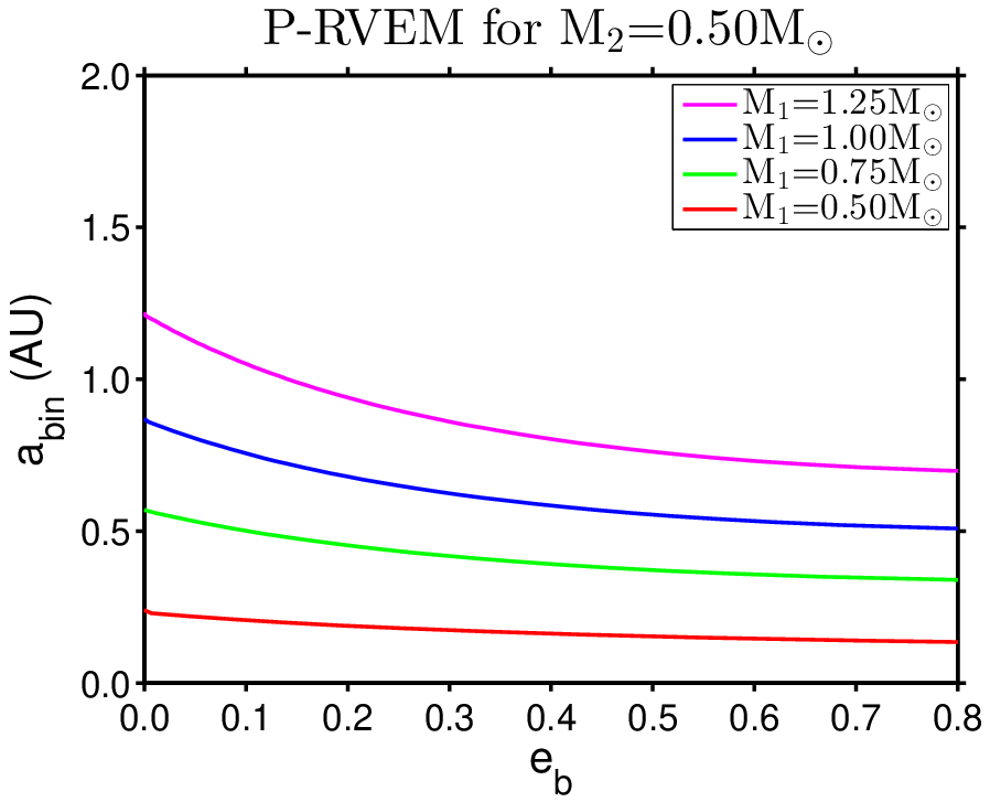
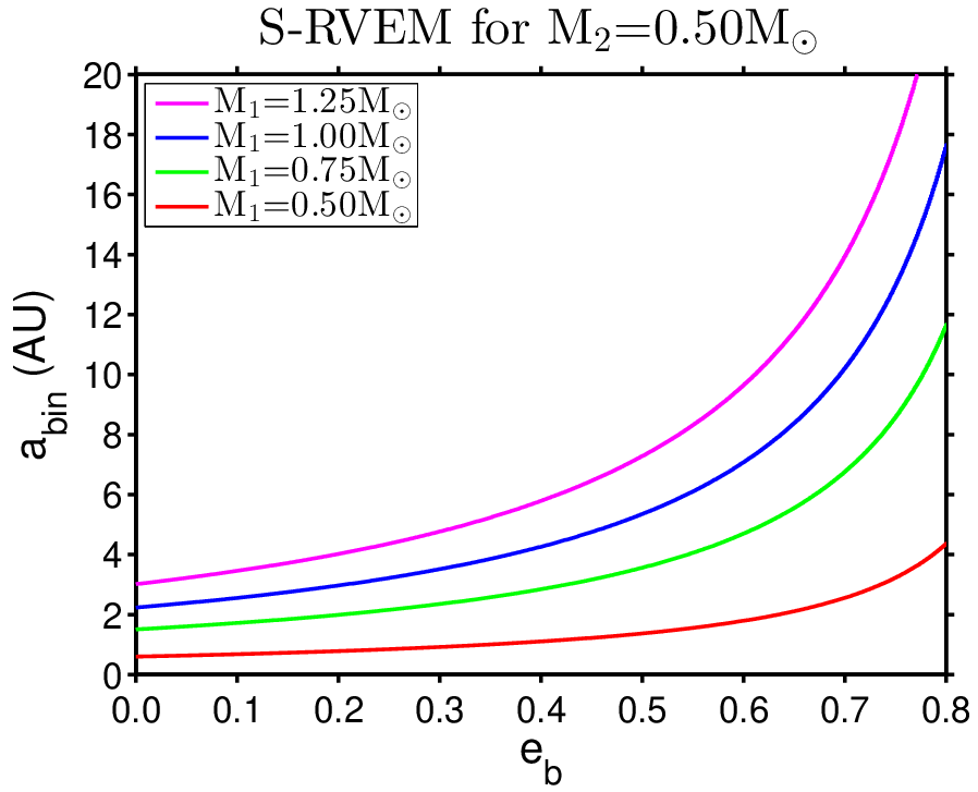
Various sets of binary systems, encompassing both systems of equal and non-equal masses, have been studied to examine the existence of their HZs based on the radiative criterion, as described by the stellar luminosities, as well as the orbital stability criterion for system planets. Information on the adopted stellar parameters, chosen for cases of theoretical main-sequence stars, are given in Table 1 and 2. Regarding the stellar HZs, we focus on the GHZ and RVEM (see Sect. 2.1) and consider stars with masses and of 0.50 , 0.75 , 1.00 , and 1.25 ; see Figures 2 to 5 for details.
For systems of masses , in case of = 0, the semi-major axis is required to be smaller than 0.97 au for the P/PT-type GHZ to exist and smaller than 1.03 au for the P/PT-type RVEM to exist. Regarding S/ST-type HZs, needs to be larger than 3.72 au and larger than 2.93 au for the GHZ and RVEM to exist, respectively. Larger eccentricities barely affect the existence of P/PT-type HZs; however, they notably affect the existence of the S/ST-type HZs. For = 0.50, is required to be larger than 8.44 au and larger than 6.66 au for S/ST-type GHZ and RVEM to exist, respectively.
Different values for the existence of P/PT and S/ST-type HZs are obtained for other kinds of equal-mass systems. For systems with masses , in case of = 0, is required to be smaller than 0.22 au for the P/PT-type GHZ to exist and smaller than 0.23 au for the P/PT-type RVEM to exist. Regarding S/ST-type HZs, needs to be larger than 0.76 au and larger than 0.60 au for the GHZ and RVEM to exist, respectively. Again, larger eccentricities barely affect the existence of P/PT-type HZs; however, they impact the existence of the S/ST-type HZs, as expected. For = 0.50, is required to be larger than 1.74 au and larger than 1.37 au for S/ST-type GHZ and RVEM to exist, respectively.
We also investigated non-equal mass systems, which generally are considered more significant than equal-mass systems. In systems of and , is required to be smaller than 0.81 au and smaller than 0.86 au for the P/PT-type GHZ and RVEM, respectively, in case of = 0. Furthermore, needs to be larger than 2.83 au and larger than 2.23 au to allow for the existence of the S/ST-type GHZ and RVEM, respectively. Again, high eccentricities barely affect the existence of P/PT-type HZs; however, they impact the existence of the S/ST-type HZs as already discussed for equal-mass systems. For = 0.50, is required to be larger than 6.78 au and larger than 5.35 au for S/ST-type GHZ and RVEM to exist, respectively.
Moreover, we also considered systems of and . The case of = 0 requires to be smaller than 1.20 au and smaller than 1.27 au for the P/PT-type GHZ and RVEM, respectively. Regarding S/ST-type HZs, is required to be larger than 4.36 au for the GHZ and larger than 3.41 au for the RVEM regarding = 0. Furthermore, is required to be larger than 10.17 au for the GHZ and larger than 8.03 au for the RVEM and = 0.50. Even higher values of are needed for both the GHZ and RVEM in case of eccentricities beyond 0.50.
In summary, the existence of P/PT-type HZs is barely affected by the eccentricity of the stellar system and solely controlled by and (or, say, and ). However, relatively large semi-major axes are required for the existence of S/ST-type HZs in highly eccentric systems. Large values of always ensure S/ST-type HZs, as in this case, the stellar habitable environments are in essence those of single stars. In non-equal mass systems with considered as fixed, the P/PT-type HZs are barely impacted compared to equal-mass systems, but higher values for are mandated for the existence of S/ST-type HZs especially for systems with high eccentricities for the binary components.
III Fitting Procedure
The main aspect of our work concerns the derivation of fitting formulae for the existence of P/PT-type HZs and S/ST-type HZs for binary systems consisting of main-sequence stars. Through applying the least-squared method, fitting is done in two steps: first, fitting versus by assuming fixed masses as reference (aimed at catching the sets of parameters where the HZs cease to exist) and, second, fitting the coefficients with stellar masses to allow the expansion of the formulae for general binary systems. In the first step, the Bayesian information criterion (BIC) and mean absolute percentage error are taken into account. The BIC is used in the second step as well for the mass fitting determination.
For P/PT-type cases, the versus fitting is done using a polynomial equation, which is
| (5) |
For S/ST-type cases, the versus fitting is done using a cubic equation, placed as exponent, which reads
| (6) |
The coefficients for selected systems are shown in Table 3. For , systems with masses of have 0.960 au for the fitting results and 0.97 au regarding the data for the P/PT-type GHZ, and 1.016 au in the fitting results and 1.03 au regarding the data for the P/PT-type RVEM to exist. For S/ST-type HZs, the fit yields 3.597 au and 2.773 au for the GHZ and RVEM, respectively, with data noted as 3.72 au and 2.93 au, respectively.
Keep to be zero, systems with , render 0.215 au, 0.230 au, 0.720 au, and 0.568 au in the fitting of P-GHZ, P-RVEM, S-GHZ, and S-RVEM, respectively. Conversely, the data based on the method as given in Sect. 2.1 are given as 0.22 au, 0.23 au, 0.76 au, and 0.60 au, respectively. In systems with , the fitting results read 0.805 au, 0.850 au, 2.702 au, and 2.109 au, respectively with as zero for P-GHZ, P-RVEM, S-GHZ, and S-RVEM, respectively. Furthermore, 0.81 au, 0.86 au, 2.83 au, and 2.23 au are the values for corresponding data. For the case of and with as zero, the results for the fitting of P-GHZ, P-RVEM, S-GHZ, and S-RVEM are given as 1.185 au, 1.253 au, 4.229 au, and 3.287 au, respectively. Here the data are 1.20 au, 1.27 au, 4.36 au, and 3.41 au, respectively, again showing very close agreement. The various fitting coefficients are listed in Table 4.
To enhance the universal applicability of the fitting formulae, we also explored the relation between the coefficents in versus fitting, and the stellar masses of the binary systems. For the coefficents in the P-type equation, is represented by
| (7) |
Furthermore, for the coefficents in the S-type equation, is represented by
| (8) |
The BIC for the cases of mass fitting are listed in Table 5. By adding terms to the equation only containing constant and linear terms of and , the BIC varies and indicates that P-type cases favor adding nothing, whereas S-type cases prefer adding and , as done as part of the process. The general fitting coefficients for P-type and S-type HZs are listed in Table 6 and 7, respectively.
Applying the calculated coefficients from stellar masses to the versus equations, fitting results are plotted as well as the data for comparison (see Fig. 3). Most of the fits are virtually indistinguishable from the data. Percent errors of the fits for selected cases are provided in Tables 8 to 10. Cases not shown here reveal similar results. In Table 10, the coefficients of determination measuring the goodness of the fit, are given for reference. The percentage errors are calculated as
| (9) |
In summary, through employing a two-step fitting procedure, fully acceptable results are obtained for the fitting equations in response to the existence of GHZ and RVEM HZs depending on the system parameters (i.e., , , , and ).
Using the fitting formulae given above (see Eqs. 5 to 8), several observed binary systems have been studied in more detail to inquire on the existence of the stellar HZs, encompassing both GHZs and RVEM HZs (see Sect. 4). Generally, the minimum for S-type HZs to exist would increase as either stellar mass increases. As for the P-type cases, the maximum is decreased with either stellar mass decreased. Thus, the maximum masses of binary components were considered for S-type HZs based on their errors for their existence, and minimum masses have been taken into account for the non-existence of HZs. In contrast, P-type HZs consider stellar minimum masses (as defined by the respective observational uncertainties) for their existence, and maximum masses for the non-existence of the HZs. As for the eccentricity, the largest eccentricity (as set by observational constraints) should be considered for the study of both S-type and P-type HZs, as it corresponds to the most adverse outcome.
IV Applications to Observed Systems
IV.1 P-type Systems
IV.1.1 Kepler-34
[39] have reported transiting circumbinary planets both regarding Kepler-34 and Kepler-35; their study also conveys detailed information about the system’s data (see Table 11). Kepler-34 has two Sun-like stars revolving around each in d, with stellar masses to be and 1.02080.0022 , respectively. The system possesses a circumbinary gas giant, i.e., somewhat less massive than Saturn, with a au semi-major axis and a eccentricity. By measuring the effective temperature and metallicity of both stars, an age between 5 and 6 Gyr has been deduced [41], based on Yonsei–Yale theoretical models of stellar evolution, and thus the stars should still be in their main-sequence stages. The semi-major axis of the binary is , and the eccentricity is . Considering the smallest possible stellar masses and largest possible eccentricity, both P-type GHZ and P-type RVEM HZs are expected to exist, noting that those should require for to be less than 0.683 au and less than 0.722 au, respectively. These criteria are fulfilled based on the observational data (see Fig. 6). [39] also pointed out that the circumbinary planet is located interior to the HZ.
IV.1.2 Kepler-35
Kepler-35 is known to have a circumbinary gas giant orbiting hosting starts on a nearly circular orbit (); see [39] for details. The planet, which has a semi-major axis to be au, is within the P-type HZs. The primary star of Kepler-35 has a mass to be , and the secondary being , with an orbital period of days. Based on the Yonsei–Yale theoretical models of stellar evolution [41], the age of this system is about 8 Gyr to 12 Gyr. This is larger than the solar age; however, based on the masses of the two stellar components, this system is still considered to be composed of main-sequence stars. The binary system has a semi-separation of au, and the eccentricity is given as . The system’s semi-major axis is clearly less than the requirements for P-type HZs to exist, which are 0.674 au and 0.712 au for the GHZ and RVEM (see Fig. 6). [39] pointed out that the circumbinary planet is located interior to the HZ.
IV.1.3 Kepler-413
Following [22], Kepler-413 has a K dwarf as primary, and a M dwarf as secondary (see Table 11). The two stars orbit each other on a nearly circular orbit, which has an eccentricity of . The orbital period is given as d. Kepler-413b, a circumbinary planet, orbiting both stars with au as semi-major axis and as eccentricity, is slightly outside of the GHZ, but insight of the RVEM. Fitting with the minimum possible stellar masses and maximum possible binary eccentricity (the most adverse choices for the existence of the circumstellar HZs), the P-type GHZ and RVEM require to be smaller than 0.572 au and 0.605 au to allow their existence. The semi-major axis of the system is au, which satisfies the requirements for circumbinary HZs to exist (see Fig. 6).
IV.1.4 Kepler-1647
Following [23], Kepler-1647b has been identified a gas giant in the eclipsing binary system Kepler-1647. The semi-major axis of the planet is 2.72050.0070 au, which is within the P-type GHZ. The primary star is estimated to be a F8 star with stellar mass as . The secondary star is similar to the Sun; it has a mass of (see Table 11). The estimated age of the system, identified as approximately 4.4 Gyr, corresponds to mid-age main-sequence. The binary orbital period is given as 11.25881790.0000013 d, with 0.12760.0002 au as binary semi-major axis and 0.16020.0004 as binary eccentricity. Taking the largest eccentricity the smallest possible stellar masses, as conveyed by the observational results, as reference, it requires to be less than 1.037 au for P-type GHZ to exist, and 1.096 au for P-type RVEM to exist. Fitting results for this system are shown in Figure 6, which clearly show that both the GHZ and RVEM are able to exist in this system.
IV.2 S-type Systems
IV.2.1 TrES-2
Following [6], TrES-2, also known as Kepler-1, consists of a planet-hosting G0V primary star with a mass of 1.05 . The planet orbits the stellar primary based on a au semi-major axis. The secondary is estimated to have a mass of 0.67 ; it is a zero-age main-sequence star. The binary separation of the system, which is estimated to be 23212 au, ensure that effects by the secondary star on the primary’s habitable environment are largely negligible; therefore, resulting in conditions akin to a single star. Thus, S-type HZs should exist around the primary star. Although the binary eccentricity is unknown, the semi-major-axis of the binary system is larger than the required value as 23.679 au for S-type GHZ and 19.303 au for S-type RVEM (see Fig. 7).
IV.2.2 KOI-1257
Following [36], KOI-1257 consists of two main-sequence stars with stellar masses of 0.990.05 and 0.700.07 , respectively (see Table 11). A 1.450.35 planet is in an S-type orbit around the primary star with 0.7720.045 as eccentricity and 0.3820.006 au as semi-major axis. The eccentricity of the binary system’s orbit is , and its semi-major axis is 5.3 au with an uncertainty of 1.3 au. In this system, the existence of S-type HZs strongly depends on the binary parameters, which are subject to notable uncertainties. At , the semi-major axis is required to be larger than 13.919 au for an S-type GHZ and 11.019 au for RVEM, which means that for this value of , there are no S-type HZs. However, for the smallest value of , given as 0.10, the requirements for the semi-major axis now read 3.899 and 3.085 au for the GHZ and RVEM, respectively, indicating the existence for both S-type types of HZs (see Fig. 7). If disregarding the observational uncertainties, the semi-major axis is given as 5.3 au. This value is larger than 5.386 au for the S-type GHZ to exist, and larger than 4.280 au for the S-type RVEM to exist.
IV.3 Comparison with Other Work
We also have compared some of our results with previous work that is based on moderately different methods for the calculations of the HZ limits. For S-type and P-type HZs, this work has been given by [15] and [17], respectively. Figure 8 shows the comparisons for the systems of Kepler-34, Kepler-35, Kepler-413, and KOI-1257. Comparisons between results based on GHZ and EVEM climate models are shown examples, with the observational uncertainties for the eccentricities taken into account. The percent differences are calculated as difference between habitability limits divided by the average.
Regarding Kepler-34, the luminosity of the primary is given as and for the secondary it is . The GHZ inner limit has a percent difference between 3.04% and 3.14%, whereas the outer limit’s difference varies between 0.777% and 0.780%. In case of RVEM, the inner limit has a minimum difference of 0.319% and a maximum difference of 0.321%. The values for the outer limit are given as 0.390% and 0.391%, respectively. Regarding Kepler-35, the luminosity of the primary is given as and for the secondary it is . The GHZ inner and outer limits have minimum percent differences of 2.94% and 0.703%, and maximum percent differences of 3.08% and 0.706%, respectively. For the RVEM climate models, the percent difference for the inner limit and outer limit are close to 0.3% and 0.5%, respectively. Regarding Kepler-413, the luminosity of the primary is given as and for the secondary it is . The inner and outer GHZ limits have percent differences ranging from 2.82% to 3.01% and from 0.562% and 0.570%. RVEM has percent difference between 1.12% and 1.22% for the inner limits, and between 0.518% and 0.519% for the outer limits.
KOI-1257, considered as an S-type system, consists of two stars with luminosities of and , respectively. The minimum and maximum percent differences of the GHZ inner limit are 3.22% and 3.73%, respectively. The value for the GHZ outer limit is approximately 0.75%. The RVEM inner limit is noted for having percent differences between 0.053% and 0.102%, whereas the RVEM out limit has a percentage difference of 0.43% with virtually no variation regarding the assumed eccentricity of the binary components. Therefore, in conclusion, our results on obtaining fitting formulae for the existence of S-type and P-type HZs are unaffected by the choice of habitability limits as available in the literature.
V Summary and Conclusions
The aim of this study was the evaluation of the mathematical constraints for the possibility of HZs in stellar binary systems — an effort of interest irrespectively of hitherto planet detections in those systems. This allowed us to deduce fitting formulae that permit — in the framework of the adopted model — a straightforward “yes/no” answer whether HZs exist. The underlying mathematical concept is based on the work of Paper I and II, which follows a comprehensive approach for the computation of habitable zones in binary systems. The latter includes (1) the consideration of a joint constraint including orbital stability and a habitable region for a putative system planet through the stellar radiative energy fluxes (RHZ) needs to be met; (2) the treatment of different types of HZs as defined for the Solar System and beyond; (3) the provision of a combined formalism for the assessment of both S-type and P-type HZs based on detailed mathematical criteria — in particular, mathematical criteria are presented for which kind of system S-type and P-type habitability is realized; and (4) applications to stellar systems in either circular or elliptical orbits. Note that previous less sophisticated fitting procedures for the existence of HZs in binary systems were given by [38].
The adopted planetary climate models follow the previous work by [20, 21], which allowed us to define the HZs referred to as GHZ and RVEM, including the definitions of the respective inner and outer limits. The inspection of the planetary orbital stability limits follows the work by [16], which expands on previous results including work by [9] and [32]. Results on the formation and dynamics of planets in dual stellar systems compared to single stars have been given by, e.g., [14] and subsequent work. The fitting formulae for the existence of the HZs, both regarding P-type and S-type HZs, obtained in our study relate the axes between the stellar binary components and an algebraic expansion for their orbital eccentricities; they target the limits where the respective HZs ceases to exist. For P-type cases, the attained algebraic expansion is of second order, and for S-type cases, it is of third order, but written as an exponential exponent. The various coefficients also depend on and , the masses of the stellar components, which ensures the comprehensive applicability of the fitting formulae. The current version of our methods is aimed at systems of main-sequence stars.
The stellar masses are assumed to range between 0.50 and 1.25 , i.e., between spectral type M0V and F6V [13, 27, e.g.,]. Thus, the respective stellar luminosities range between 0.036 and 2.15 . Therefore, notwithstanding late-type red dwarfs, the kind of stars for which our approach is applicable comprises more than 95% of main-sequence stars [24, 25, 2, e.g.,]. Furthermore, detailed tests for our fitting formulae demonstrate that their accuracy compared to the exact results based on the solutions for the underlying quartic equations (see Papers I and II) is better than 5% in most cases, noting that the least accurate results are found for systems of high eccentricity, i.e., . In fact, for the vast majority of cases the accuracy of the fitting formulae is found to be about 1% or 2%.
Our method is particularly useful for the quick assessment of observed systems with relatively large (or poorly known) uncertainties in , , , and , while noting that the latter can play a decisive role regarding whether or not S-type or P-type HZs exist. To demonstrate the applicability of our method, we explored the existence of P-type HZs for Kepler-34, Kepler-35, Kepler-413, and Kepler-1647 and S-type HZs for TrES-2 and KOI-1257. Observational uncertainties of the various system parameters have been considered as well, which can be relevant for the outcome. A good example is KOI-1257, where the existence of the S-type HZ is strongly affected by the values for both the semi-major axis and the eccentricity of the stellar motion, which are somewhat uncertain. On the other hand, we found that all P-type systems considered possess P-type HZs irrespectively of the uncertainties in the relevant observational parameters. These results are also unaffected by the planetary climate models.
Generally, the likelihood for the existence of HZs is relatively high for low values of the , but relatively small, or virtually non-existing, for high values of the . Moreover, the likelihood if a HZs can exist is also increased if RVEM-type HZs are considered rather than GHZ-type HZs, as expected. The fact that high values for decisively reduce the possibility of S-type habitability has previously been pointed out by, e.g., [4]. Our future work will also consider stellar systems of stars other than main-sequence components and also take into account future advances about planetary climate models, including the impact of planetary masses and atmospheric structures.
References
- [1] Bazsó, Á., Pilat-Lohinger, E., Eggl, S., Funk, B., Bancelin, D., & Rau, G. 2017, MNRAS, 466, 1555
- [2] Chabrier, G. 2003, PASP, 115, 763
- [3] Cuntz, M. 2014, ApJ, 780, 14 [Paper I]
- [4] Cuntz, M. 2015, ApJ, 798, 101 [Paper II]
- [5] Cuntz, M., & Bruntz, R. 2014, in Cool Stars, Stellar Systems, and the Sun: 18th Cambridge Workshop, ed. G. van Belle & H. Harris (Flagstaff: Lowell Observatory), p. 831
- [6] Daemgen, S., Hormuth, F., Brandner, W., Bergfors, C., Janson, M., Hippler, S., & Henning, T. 2009, A&A, 498, 567
- [7] Duquennoy, A., & Mayor, M. 1991, A&A, 248, 485
- [8] Dvorak, R. 1982, OAWMN, 191, 423
- [9] Dvorak, R. 1986, A&A, 167, 379
- [10] Eggenberger, A., Udry, S., & Mayor, M. 2004, A&A, 417, 353
- [11] Eggl, S., Pilat-Lohinger, E., Georgakarakos, N., Gyergyovits, M., & Funk, B. 2012, ApJ, 752, 74
- [12] Eggl, S., Pilat-Lohinger, E., Funk, B., Georgakarakos, N., & Haghighipour, N. 2013, MNRAS, 428, 3104
- [13] Gray, D. F. 2005, The Observation and Analysis of Stellar Photospheres, 2nd edn., Cambridge University Press, Cambridge
- [14] Haghighipour, N. 2008, in Exoplanets, Springer Praxis Books, Chichester, UK, p. 223
- [15] Haghighipour, N., & Kaltenegger, L. 2013, ApJ, 777, 166
- [16] Holman, M. J., & Wiegert, P. A. 1999, AJ, 117, 621
- [17] Kaltenegger, L., & Haghighipour, N. 2013, ApJ, 777, 165
- [18] Kane, S. R., & Hinkel, N. R. 2013, ApJ, 762, 7
- [19] Kasting, J. F., Whitmire, D. P., & Reynolds, R. T. 1993, Icarus, 101, 108
- [20] Kopparapu, R. K., Ramirez, R., Kasting, J. F., et al. 2013, ApJ, 765, 131; Erratum 770, 82
- [21] Kopparapu, R. K., Ramirez, R. M., SchottelKotte, J., et al. 2014, ApJ, 787, L29
- [22] Kostov, V. B., McCullough, P. R., Carter, J. A., et al. 2014, ApJ, 784, 14; Erratum 787, 93
- [23] Kostov, V. B., Orosz, J. A., Welsh, W. F., et al. 2016, ApJ, 827, 86
- [24] Kroupa, P. 2001, MNRAS, 322, 231
- [25] Kroupa, P. 2002, Science, 295, 82
- [26] Ma, B., Ge, J., Wolszczan, A., et al. 2016, AJ, 152, 112
- [27] Mann, A. W., Gaidos, E., & Ansdell, M. 2013, ApJ, 779, 188
- [28] Müller, T. W. A., & Haghighipour, N. 2014, ApJ, 782, 26
- [29] Ortiz, M., Gandolfi, D., Reffert, S., et al. 2015, A&A, 573, L6
- [30] Patience, J., White, R. J., Ghez, A. M., et al. 2002, ApJ, 581, 654
- [31] Pilat-Lohinger, E., & Dvorak, R. 2002, CMDA, 82, 143
- [32] Rabl, G., & Dvorak, R. 1988, A&A, 191, 385
- [33] Raghavan, D., Henry, T. J., Mason, B. D., et al. 2006, ApJ, 646, 523
- [34] Raghavan, D., McAlister, H. A., Henry, T. J., et al. 2010, ApJS, 190, 1
- [35] Roell, T., Neuhäuser, R., Seifahrt, A., & Mugrauer, M. 2012, A&A, 542, A92
- [36] Santerne, A., Hébrard, G., Deleuil, M., et al. 2014, A&A, A571, 37
- [37] Underwood, D. R., Jones, B. W., & Sleep, P. N. 2003, IJAsB, 2, 289
- [38] Wang, Zh., & Cuntz, M. 2016, in The 19th Cambridge Workshop on Cool Stars, Stellar Systems, and the Sun, ed. G. A. Feiden, 7, zenodo, doi:10.5281/zenodo.154425
- [39] Welsh, W. F., Orosz, J. A., Carter, J. A., et al. 2012, Nature, 481, 475
- [40] Welsh, W. F., Orosz, J. A.; Short, D. R., et al. 2015, ApJ, 809, 26
- [41] Yi, S., Demarque, P., Kim, Y.-C., Lee, Y.-W., Ree, C. H., Lejeune, T., & Barnes, S. 2001, ApJS, 136, 417
- [42] Zuluaga, J. I., Mason, P. A., & Cuartas-Restrepo, P. A. 2016, ApJ, 818, 160
 |
 |

 |

 |

 |

 |

 |

 |

 |

 |

 |

 |

 |

 |

 |
| Description | Indices | Models | This work | ||
|---|---|---|---|---|---|
| … | Kas93 | Kop1314 | … | ||
| … | … | 5700 K | 5780 K | 5780 K | … |
| … | … | (au) | (au) | (au) | … |
| Recent Venus | 1 | 0.75 | 0.77 | 0.750 | RVEM Inner Limit |
| Runaway greenhouse effect | 2 | 0.84 | 0.86 | 0.950 | GHZ Inner Limit |
| Moist greenhouse effect | 3 | 0.95 | 0.97 | 0.993 | … |
| Earth-equivalent position | 0 | 0.993 | 1 | 1 | … |
| First CO2 condensation | 4 | 1.37 | 1.40 | … | … |
| Maximum greenhouse effect | 5 | 1.67 | 1.71 | 1.676 | GHZ Outer Limit |
| Early Mars | 6 | 1.77 | 1.81 | 1.768 | RVEM Outer Limit |
| Spectral Type | ||||
|---|---|---|---|---|
| () | … | (K) | () | () |
| 1.25 | F6V | 6257 | 1.253 | 2.154 |
| 1.00 | G2V | 5780 | 1.000 | 1.0000 |
| 0.75 | K2V | 5104 | 0.766 | 0.3568 |
| 0.50 | M0V | 3664 | 0.472 | 0.03593 |
Note. — Adopted from Paper I and II.
| BIC | Linear | Quadratic | Cubic | Quartic |
|---|---|---|---|---|
| PGHZ | 287.28 | 418.18 | 538.74 | 627.83 |
| PRVEM | 295.91 | 432.93 | 564.12 | 642.10 |
| SGHZ | 7915.7 | 12327 | 16347 | 19794 |
| SRVEM | 7422.6 | 11599 | 15395 | 18840 |
Note. — The case of is given as an example for the determination of the versus fitting. For all S-type results, the logarithm of is applied. The mean absolute percentage error (MAPE) is calculated as well, and a 2% threshold is used. The BICs are found to decrease as the orders of the equations increase from 1 to 3 for all cases indicating that it is acceptable to have cubic equations. Lowest order equations satisfy the MAPE requirement are chosen for less complexity.
| Model | Coefficient | Case 1 | Case 2 | Case 3 | Case 4 |
|---|---|---|---|---|---|
| P-GHZ | 0.215 | 0.805 | 0.805 | 1.185 | |
| … | 0.205 | 0.933 | 0.933 | 1.302 | |
| … | 0.123 | 0.716 | 0.716 | 0.949 | |
| P-RVEM | 0.230 | 0.850 | 0.850 | 1.253 | |
| … | 0.228 | 0.957 | 0.957 | 1.371 | |
| … | 0.146 | 0.695 | 0.695 | 0.992 | |
| S-GHZ | 0.328 | 0.994 | 0.994 | 1.442 | |
| … | 2.169 | 2.088 | 2.088 | 1.601 | |
| … | 3.046 | 2.497 | 2.497 | 0.956 | |
| … | 4.346 | 3.901 | 3.901 | 2.506 | |
| S-RVEM | 0.566 | 0.746 | 0.746 | 1.19 | |
| … | 2.177 | 2.256 | 2.256 | 1.844 | |
| … | 3.065 | 3.024 | 3.024 | 1.787 | |
| … | 4.359 | 4.349 | 4.349 | 3.275 |
Note. — Case 1: ; Case 2: , ; Case 3: ; Case 4: , .
| Model | BIC | Linear to and | Adding and | Adding and | Adding and | Adding and | Adding and |
|---|---|---|---|---|---|---|---|
| PGHZ | Constant | 80.90 | 75.94 | 76.06 | 75.21 | 81.84 | 75.94 |
| … | Coef. of term | 71.59 | 67.34 | 68.70 | 68.32 | 70.66 | 67.67 |
| … | Coef. of term | 74.75 | 69.81 | 71.19 | 70.77 | 74.42 | 69.65 |
| PRVEM | Constant | 78.20 | 71.14 | 75.24 | 75.76 | 76.26 | 74.80 |
| … | Coef. of term | 68.41 | 66.79 | 68.86 | 64.14 | 65.96 | 63.09 |
| … | Coef. of term | 64.78 | 66.50 | 63.89 | 65.04 | 61.58 | 63.44 |
| Total | … | 438.64 | 417.51 | 423.94 | 419.25 | 430.73 | 414.59 |
| SGHZ | Constant | 31.68 | 48.70 | 49.40 | 34.20 | 66.87 | 28.96 |
| … | Coef. of term | 41.16 | 51.60 | 51.75 | 38.90 | 57.37 | 37.18 |
| … | Coef. of term | 18.43 | 30.32 | 30.15 | 17.85 | 35.97 | 14.79 |
| … | Coef. of term | 20.18 | 34.76 | 34.62 | 20.22 | 39.84 | 16.63 |
| SRVEM | Constant | 31.78 | 46.96 | 47.44 | 33.85 | 69.32 | 28.97 |
| … | Coef. of term | 36.27 | 53.25 | 54.17 | 38.71 | 65.40 | 33.20 |
| … | Coef. of term | 13.49 | 28.14 | 30.12 | 17.55 | 36.86 | 10.94 |
| … | Coef. of term | 16.11 | 30.85 | 32.98 | 20.42 | 39.04 | 13.67 |
| Total | … | 209.11 | 324.58 | 330.62 | 221.70 | 410.68 | 184.34 |
Note. — The coefficients from the versus fitting are further fitted based on an equation linear in the stellar masses. Additional terms are added by checking the BIC. The smallest BIC in each line is given in bold font. The total BIC values in each column are compared. For P-type, adding nothing is preferred, whereas for S-type, adding and turns out to be the best choice.
| Model | Coefficient | |||
|---|---|---|---|---|
| P-GHZ | 0.541 | 1.201 | 0.318 | |
| … | 0.541 | 1.504 | 0.012 | |
| … | 0.345 | 1.219 | 0.275 | |
| P-RVEM | 0.570 | 1.266 | 0.338 | |
| … | 0.578 | 1.553 | 0.036 | |
| … | 0.384 | 1.213 | 0.187 |
| Model | Coefficient | |||||
|---|---|---|---|---|---|---|
| S-GHZ | 5.871 | 16.88 | 0.499 | 14.932 | 4.688 | |
| … | 0.002 | 8.934 | 0.464 | 9.835 | 3.160 | |
| … | 2.852 | 24.115 | 1.018 | 26.776 | 8.352 | |
| … | 0.414 | 19.528 | 0.991 | 21.219 | 6.371 | |
| S-RVEM | 6.354 | 17.873 | 0.500 | 16.177 | 5.168 | |
| … | 3.311 | 4.510 | 0.461 | 7.080 | 3.349 | |
| … | 7.312 | 17.184 | 0.954 | 25.040 | 11.499 | |
| … | 8.047 | 14.891 | 0.883 | 21.811 | 10.027 |
| … | P-GHZ | P-RVEM | S-GHZ | S-RVEM | P-GHZ | P-RVEM | S-GHZ | S-RVEM |
|---|---|---|---|---|---|---|---|---|
| 0.0 | 0.53% | 0.17% | 4.96% | 6.36% | 0.58% | 0.02% | 2.71% | 4.09% |
| 0.1 | 2.28% | 2.21% | 0.67% | 0.44% | 2.25% | 2.20% | 2.21% | 2.46% |
| 0.2 | 2.66% | 2.46% | 0.11% | 0.89% | 2.27% | 2.33% | 3.26% | 4.09% |
| 0.3 | 2.20% | 2.04% | 0.70% | 0.09% | 1.31% | 1.38% | 2.14% | 2.80% |
| 0.4 | 1.59% | 1.40% | 1.59% | 1.52% | 0.33% | 0.19% | 0.66% | 0.86% |
| 0.5 | 1.27% | 1.11% | 1.82% | 2.20% | 0.07% | 0.40% | 0.18% | 0.20% |
| 0.6 | 1.59% | 1.50% | 0.98% | 1.40% | 1.20% | 0.16% | 1.13% | 0.62% |
| 0.7 | 2.99% | 2.98% | 0.67% | 0.08% | 4.13% | 2.32% | 2.27% | 2.59% |
| 0.8 | 5.78% | 5.82% | … | … | 9.26% | 6.34% | … | 0.92% |
| … | P-GHZ | P-RVEM | S-GHZ | S-RVEM | P-GHZ | P-RVEM | S-GHZ | S-RVEM |
|---|---|---|---|---|---|---|---|---|
| 0.0 | 3.48% | 3.47% | 2.97% | 3.36% | 0.33% | 0.00% | 5.41% | 6.08% |
| 0.1 | 1.87% | 1.85% | 3.77% | 3.80% | 1.82% | 2.05% | 0.58% | 0.59% |
| 0.2 | 2.02% | 1.95% | 5.40% | 5.52% | 2.50% | 2.74% | 2.30% | 2.26% |
| 0.3 | 2.96% | 2.92% | 4.04% | 4.12% | 2.37% | 2.53% | 1.21% | 1.09% |
| 0.4 | 3.99% | 4.14% | 1.91% | 2.12% | 2.00% | 1.94% | 0.65% | 0.75% |
| 0.5 | 4.38% | 4.83% | 0.87% | 0.98% | 1.80% | 1.49% | 1.60% | 1.59% |
| 0.6 | 3.58% | 4.52% | 1.63% | 1.63% | 2.25% | 1.47% | 0.67% | 0.65% |
| 0.7 | 1.29% | 2.88% | 3.43% | 3.34% | 3.60% | 2.33% | 1.24% | 1.12% |
| 0.8 | 2.58% | 0.45% | 0.34% | 0.46% | 6.10% | 4.56% | 2.27% | 2.86% |
| Systems | P-GHZ | P-RVEM | S-GHZ | S-RVEM |
|---|---|---|---|---|
| 0.9976 | 0.9975 | 0.9967 | 0.9969 | |
| 0.9795 | 0.9758 | 0.9999 | 0.9997 | |
| 0.9919 | 0.9929 | 0.9990 | 0.9991 | |
| 0.9954 | 0.9940 | 0.9991 | 0.9990 | |
| 0.9803 | 0.9820 | 0.9990 | 0.9984 | |
| 0.9970 | 0.9963 | 0.9994 | 0.9988 | |
| 0.9849 | 0.9853 | 0.9985 | 0.9978 | |
| 0.9876 | 0.9861 | 0.9947 | 0.9954 | |
| 0.9619 | 0.9632 | 0.9960 | 0.9962 | |
| 0.9780 | 0.9834 | 0.9991 | 0.9991 |