Representation of complex probabilities and complex Gibbs sampling

Let $P(g)$ be a complex probability defined on a matrix group $G=\{e^{-i\vec{a}\cdot\vec{T}},~\vec{a}\in\mathbb{R}^{m}\}$. The observables can be analytically extended to the complexified group $\tilde{G}=\{e^{-i\vec{a}\cdot\vec{T}},~\vec{a}\in\mathbb{C}^{m}\}$, Haar measures can be adopted on $G$ and $\tilde{G}$ and representations can be defined as before.

The two-branch scheme can be adapted to the present case: Letting  $G_{I}\equiv\{e^{-i\vec{a}\cdot\vec{T}},~\vec{a}\in i\mathbb{R}^{m}\}$,

where $A(gh^{-1})$, $A(gh)\,$ refer to the analytical extension in $\tilde{G}$. So the Monte Carlo sampling is carried out using the real and positive weights $Q_{\pm}(g)$ defined on $G$.

To do the matching in Eq. (15), $P$ and $Q_{\pm}$ are expanded as a linear combination of group representations (generalizing the Fourier modes of ${\mathrm{U}}(1)$). For instance in ${\mathrm{U}}(N)$, for

(not the most general case) one finds the solution, choosing $\,h=\mathrm{diag}(\omega_{1},\ldots,\omega_{N})$   ($\omega_{i}>0$),

where  $\Omega_{j_{1},\ldots,j_{n}}\equiv\omega_{j_{1}}\!\cdots\omega_{j_{n}}$. Once again, for sufficiently large $h\,$ the constant (group singlet) mode dominates and $Q_{\pm}>0$. (The constant mode is to be added separately both in Eq. (17) and in Eq. (18).)

As an example, a two-branch representation on $\mathrm{SU}(2)$ for  $P(g)=1+\beta\,\mathrm{tr}(\sigma_{3}\,g)$  is

$Q_{+}(g)$ is displayed in figure 3, using $g=a_{0}-i\vec{a}\cdot\vec{\sigma}$,  and  $(a_{0},\vec{a})\in\mathrm{S}^{3}$.

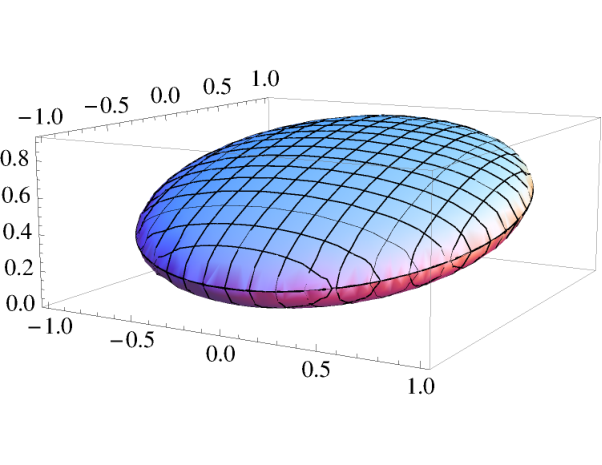
As it would be expected subtleties arise in the non-Abelian case: regardless of the choice of $h$, certain components (singlet with respect to $h\,$) will remain unchanged (would have $\Omega=1$ in Eq. (18)). Equation (15) can only be fulfilled if $P$ is real along those components. For them a different element $h^{\,\prime}\in G_{I}$ has to be applied, subject to the condition

The construction of direct representations just discussed becomes rapidly inviable as the dimension of the manifold increases. This suggests a heat bath approach. As in the standard Gibbs sampling, each variable is updated in turn, but, since the conditional probability is complex, a representation of it is used instead:

where $\rho_{\text{rep}}(z_{i}^{\prime}|\{z_{j\not=i}\})$  is a representation (with respect to $z_{i}^{\prime}$) of the conditional probability

By construction only one-variable representations are needed, however, the method relies on the analytical extension of $P({\vec{x}})$, just like CLE. Furthermore convergence to a representation of $P(x)$ is not guaranteed as standard Markovian chain theorems do not apply. Also, there is a potential problem from zeroes of the marginal probabilities $P(z_{1},\ldots,\widehat{z_{i}},\ldots,z_{n})$.

To see the performance of the method we have studied a concrete model [16], namely, a complex action in a $d$-dimensional periodic lattice

with conditional probability $P[\phi_{x}|\{\phi_{x^{\prime}\not=x}\}]\,\propto\,e^{-\lambda\phi_{x}^{4}-\phi_{x}^{2}-\beta\,\phi_{x}\sum_{\mu=1}^{d}(\phi_{x+\hat{\mu}}+\phi_{x-\hat{\mu}})}.$ In the free case ($\lambda=0$), this conditional probability is a displaced real Gaussian and the marginal probability has no zeroes. The method works alright for a bounded region of the $\beta$ plane ($e^{-S}$ is normalizable for bounded $\mathrm{Re}(\beta)$).

We further apply the complex Gibbs sampling approach for $\lambda=1$ and imaginary $\beta$. Some checks from $T$-matrix calculations, for $d=1$ only, show that the method works up to $|\beta|\approx 1$.

For higher dimensions we have used checks from virial (or Schwinger-Dyson) relations

The choices $A=\phi_{x}$ and $A=\phi_{x+\hat{\mu}}\,$, give rise to four observables $O_{1,2}$ and $I_{1,2}$ such that $\langle I_{1}\rangle=\langle I_{2}\rangle=0.$ These observables are computed using Monte Carlo and results are displayed in table 1. Reweighting and complex Langevin results are also displayed for comparison.

As expected reweighting stops working for the larger lattices. Complex heat bath works rather well for any lattice size for moderated couplings although several technical issues arise, including the need of a cutoff and filtering of rare (but catastrophic) cases (see [16] for details).

Some small bias is observed in $\langle I_{1}\rangle$ (which ought to be zero). Likely, this is rooted in a real weakness of the method, related to the presence of zeroes in the marginal probabilities. To analyze this, let us assume, in a two-variable setting, that the current distribution $\rho$ is a proper representation, $\langle A\rangle_{\rho}=\langle A\rangle_{P}$. One would like the Gibbs update to preserve this property. A Gibbs update $(z_{1},z_{2})\to(z_{1}^{\prime},z_{2})$, produces a new distribution $\rho^{\prime}$. Using the representation property one has:

So spurious contributions may arise from poles in $1/P(z_{2})$. This idea is fully sustained by a detailed analysis of $P(x_{1},x_{2})=(1+\beta\cos(x_{1}))(1+\beta\cos(x_{2}))(1+\beta\cos(x_{1}-x_{2})).$ A bias is found whenever $[-Y,Y]$ contains the zero of $P(z_{2})\sim 1+\frac{1}{2}\beta^{2}\cos(z_{2})$, and this cannot be prevented for sufficiently large $\beta$  ($Y$ increases and the zero $z_{2}$ decreases).

To have a robust method it is mandatory to find a way to remove the spurious contributions from the poles in $1/P(z_{1},\ldots,\widehat{z_{i}},\ldots,z_{n})$, when they exist. No such technique is available yet. On the other hand, it is not hard to monitor on-the-flight whether the marginal probabilities stay away from zero during the Markovian chain. This is displayed in figure 4.

References

- (1) P. Hasenfratz, F. Karsch, Phys. Lett. 125B, 308 (1983)
- (2) M. Troyer, U.J. Wiese, Phys. Rev. Lett. 94, 170201 (2005), cond-mat/0408370
- (3) G. Parisi, Phys. Lett. 131B, 393 (1983)
- (4) J.R. Klauder, Acta Phys. Austriaca Suppl. 25, 251 (1983)
- (5) G. Aarts, E. Seiler, I.O. Stamatescu, Phys. Rev. D81, 054508 (2010), 0912.3360
- (6) K. Nagata, J. Nishimura, S. Shimasaki, PTEP 2016, 013B01 (2016), 1508.02377
- (7) L.L. Salcedo, Phys. Rev. D94, 114505 (2016), 1611.06390
- (8) E. Seiler, Status of Complex Langevin, in Proceedings, 35th International Symposium on Lattice Field Theory (Lattice2017): Granada, Spain, to appear in EPJ Web Conf.
- (9) M. Cristoforetti, F. Di Renzo, L. Scorzato (AuroraScience), Phys. Rev. D86, 074506 (2012)
- (10) A. Alexandru, G. Basar, P.F. Bedaque, G.W. Ridgway, N.C. Warrington, JHEP 05, 053 (2016)
- (11) J. Bloch, Phys. Rev. Lett. 107, 132002 (2011), 1103.3467
- (12) N. Prokof’ev, B. Svistunov, Phys. Rev. Lett. 87, 160601 (2001)
- (13) J. Wosiek, JHEP 04, 146 (2016), 1511.09114
- (14) L.L. Salcedo, J. Math. Phys. 38, 1710 (1997), hep-lat/9607044
- (15) L.L. Salcedo, J. Phys. A40, 9399 (2007), 0706.4359
- (16) L.L. Salcedo, Phys. Rev. D94, 074503 (2016), 1510.09064
- (17) E. Seiler, J. Wosiek (2017), 1702.06012
- (18) E. Seiler, J. Wosiek, Positive Representations of a Class of Complex, Periodic Measures, in Proceedings, 35th International Symposium on Lattice Field Theory (Lattice2017): Granada, Spain, to appear in EPJ Web Conf.