Constant-Length Labeling Schemes for
Deterministic Radio Broadcast
Abstract
Broadcast is one of the fundamental network communication primitives. One node of a network, called the source, has a message that has to be learned by all other nodes. We consider broadcast in radio networks, modeled as simple undirected connected graphs with a distinguished source. Nodes communicate in synchronous rounds. In each round, a node can either transmit a message to all its neighbours, or stay silent and listen. At the receiving end, a node hears a message from a neighbour in a given round if listens in this round and if is its only neighbour that transmits in this round. If more than one neighbour of a node transmits in a given round, we say that a collision occurs at . We do not assume collision detection: in case of a collision, node does not hear anything (except the background noise that it also hears when no neighbour transmits).
We are interested in the feasibility of deterministic broadcast in radio networks. If nodes of the network do not have any labels, deterministic broadcast is impossible even in the four-cycle. On the other hand, if all nodes have distinct labels, then broadcast can be carried out, e.g., in a round-robin fashion, and hence -bit labels are sufficient for this task in -node networks. In fact, -bit labels, where is the maximum degree, are enough to broadcast successfully. Hence, it is natural to ask if very short labels are sufficient for broadcast. Our main result is a positive answer to this question. We show that every radio network can be labeled using 2 bits in such a way that broadcast can be accomplished by some universal deterministic algorithm that does not know the network topology nor any bound on its size. Moreover, at the expense of an extra bit in the labels, we can get the following additional strong property of our algorithm: there exists a common round in which all nodes know that broadcast has been completed. Finally, we show that 3-bit labels are also sufficient to solve both versions of broadcast in the case where the labeling scheme does not know which node is the source.
keywords: broadcast, radio network, labeling scheme, feasibility
1 Introduction
1.1 The model and the problem
Broadcast is one of the fundamental and most extensively studied network communication primitives. One node of a network, called the source, has a message that has to be learned by all other nodes. We consider broadcast in radio networks, modeled as simple undirected connected graphs with a distinguished source. In the sequel, we use the word graph in this sense, and we consider the notions of network and graph as synonyms. Nodes communicate in synchronous rounds. Throughout the paper, round numbers refer to the local time at the source, which can differ from the local time at other nodes. In each round, a node can either transmit a message to all its neighbours, or stay silent and listen. At the receiving end, a node hears a message from a neighbour in a given round if listens in this round and if is its only neighbour that transmits in this round. If more than one neighbour of a node transmits in a given round, we say that a collision occurs at . We do not assume collision detection: in case of a collision, node does not hear anything (except the background noise that it also hears when no neighbour transmits). If collision detection is available, broadcast is trivially feasible, even in anonymous networks: consecutive bits of the source message can be transmitted by a sequence of silent and noisy rounds, cf. [7], using silence as 0 and a message or collision as 1.
We are interested in the feasibility of deterministic broadcast in radio networks. If the nodes of the network do not have any labels (or all have the same label), then deterministic broadcast is impossible even in the four-cycle. Indeed, the two neighbours of the source must behave identically, i.e., transmit in exactly the same rounds, and hence, due to collisions, the fourth node can never hear a message. On the other hand, if all nodes have distinct labels, then broadcast can be carried out, e.g., in a round-robin fashion, and hence -bit labels are sufficient for this task in -node networks. It is easy to see that, by using a proper colouring of the square of the graph, -bit labels, where is the maximum degree, are enough to successfully broadcast. Hence, it is natural to ask if very short labels are sufficient for deterministic broadcast. In particular, is it possible to broadcast in every radio network using labels of constant length? Below we formalize our question.
A labeling scheme for a network represented by a graph is any function from the set of nodes into the set of finite binary strings. The string is called the label of the node . Note that labels assigned by a labeling scheme are not necessarily distinct. The length of a labeling scheme is the maximum length of any label assigned by it.
Consider all graphs , each labeled by some labeling scheme, with a distinguished source . Initially, each node knows only its own label, and the source has a message. A universal deterministic broadcast algorithm works in synchronous rounds as follows. In each round, every node makes a decision if it should transmit or listen. This decision is based only on the current history of the node, which consists of the label of the node and the sequence of messages heard by the node so far. In particular, the decision does not depend on any knowledge of the graph , including its size. However, the labeling scheme can use complete knowledge of the graph. Upon completion of the algorithm, all nodes should have the source message. For simplicity, we assume that when a node transmits, it can transmit its entire history (which may include the source message). However, in our algorithm, much smaller messages will suffice: they consist of either the source message or a constant-size “stay” message.
We also consider a variant of the above problem called acknowledged broadcast, which requires that the source node eventually knows that all nodes have received the source message. In our algorithm for this version of the problem, each transmitted message additionally contains a binary string of length , where is the size of the graph. One of the roles of this string is to implement a global clock. More specifically, in our algorithms, a node transmits only in response to receiving a message, and hence the current round number (which is the current local round number at the source node) can be maintained by including it in each transmitted message and incrementing it appropriately. Using our algorithm for acknowledged broadcast, we can ensure that there is a common round in which all nodes know that the broadcast of the source’s message has been completed.
Using the above terminology, our central question can be formulated as follows:
Does there exist a universal deterministic (acknowledged) broadcast algorithm using labeling schemes of constant length for all radio networks?
The above question can be seen in the framework of algorithms using informative labeling schemes, or equivalently, algorithms with advice [1, 11, 14, 16, 17, 19, 18, 20, 21, 26, 30, 31, 32, 38]. When advice is given to nodes, two variations are considered: either the binary string given to nodes is the same for all of them [27] or different strings are given to different nodes [20, 21], as in the case of the present paper. If strings may be different, they can be considered as labels assigned to nodes. Several authors have studied the minimum amount of advice (i.e. label length) required to solve certain network problems. The framework of advice or labeling schemes is useful for quantifying the amount of information used to solve a network problem, regardless of the type of information that is provided.
1.2 Our results
Our main contribution is a positive answer to our central question. For every radio network, we construct labeling schemes of constant length, and we design universal deterministic broadcast and acknowledged broadcast algorithms using these schemes. For the broadcast task, our labeling schemes have length 2, while for acknowledged broadcast, our labeling schemes have length 3. In the more difficult situation where the source node is not known at the time of labeling, our labeling scheme has length 3 (for both versions of broadcast).
The importance of our result can be shown in the following scenario. Suppose that transmitting devices that form a radio network are already deployed, and only a central monitor knows the location and the transmitting range of each of them, thus knowing the topology of the resulting network. This could be applicable in an Internet of Things network in a business or industrial complex. One node of this network has to broadcast many consecutive messages to all other nodes. Then the monitor can assign very short labels to the devices, enabling multiple executions of the universal broadcast. The fact that labels can be very short may be crucial in situations when nodes of the network are weak and simple devices with very limited memory. Moreover, the fact that we can also do acknowledged broadcast in this situation permits the source to send the next message only after all nodes received the preceding one. Our work is also relevant in the context of Software-Defined Networks (SDNs) where the central controller assigns to each network device a role, i.e., a forwarding behaviour. Our solution gives an efficient implementation for broadcast that requires very few roles as well as simple forwarding rules.
1.3 Related work
Algorithmic problems in radio networks modeled as graphs were studied for such tasks as broadcast [9, 24], gossiping [9, 23] and leader election [36]. In some cases [9, 23], the topology of the network was unknown, in others [24], nodes were assumed to have a labeled map of the network and could situate themselves in it.
For the broadcast task, most of the papers represented radio networks as arbitrary (undirected or directed) graphs. Models used in the literature about algorithmic aspects of radio communication, starting from [5], differ mostly in the amount of information about the network that is assumed available to nodes. However, assumptions about this knowledge concern particular items of information, such as the knowledge of the size of the network, its diameter, maximum degree, or some neighbourhood around the nodes. In this paper, we adopt the approach of limiting the total number of bits available to nodes, regardless of their meaning.
Deterministic centralized broadcast assuming complete knowledge of the network was considered in [6], where a polynomial-time algorithm constructing a -time broadcast scheme was given for all -node networks of radius . Subsequent improvements by many authors [15, 22, 24] were followed by the polynomial-time algorithm from [35] constructing a -time broadcast scheme, which is optimal. On the other hand, in [2], the authors proved the existence of a family of -node networks of radius 2 for which any broadcast algorithm requires time . The “minimal dominating sets” that appear in our work were used under the name “minimal covering sets” in the context of deterministic centralized broadcast and gossiping assuming complete knowledge of the network [24, 25].
One of the first papers to study deterministic distributed broadcast in radio networks whose nodes have only limited knowledge of the topology was [3]. The authors assumed that nodes know only their own identifier and the identifiers of their neighbours. Many authors [4, 7, 8, 9, 10] studied deterministic distributed broadcast in radio networks under the assumption that nodes know only their own identifier (but not the identifiers of their neighbours). In [7], the authors gave a broadcast algorithm working in time for undirected -node graphs, assuming that the nodes can transmit spontaneously before getting the source message. For this model, a matching lower bound on deterministic broadcast time was proved in [34], even for the class of networks of constant diameter. Increasingly faster broadcast algorithms working for arbitrary radio networks were constructed, the currently fastest being the algorithm from [12]. On the other hand, in [10], a lower bound on broadcast time was proved for -node networks of radius .
Randomized broadcast algorithms in radio networks have also been studied [3, 37]. For these algorithms, no topological knowledge of the network and no labels of nodes were assumed. In [3], the authors showed a randomized broadcast algorithm running in expected time . In [37], it was shown that for any randomized broadcast algorithm and parameters , there exists an -node network of radius requiring expected time to execute this algorithm. It should be noted that the lower bound from [2], for some networks of radius 2, holds for randomized algorithms as well. A randomized algorithm working in expected time , and thus matching the above lower bounds, was presented in [13, 33].
Many papers [1, 11, 14, 16, 17, 19, 18, 20, 21, 26, 31, 32, 38] have proposed algorithms to solve network tasks more efficiently by providing arbitrary information to nodes of the network or mobile agents circulating in it. These are known as algorithms using informative labeling schemes or algorithms with advice. Most relevant to this paper are those concerning radio networks. In [30], the authors considered the set of radio networks in which it is possible to perform broadcast in constant time when each node has complete knowledge of the network. They proved that bits of advice are sufficient for performing broadcast in constant time in such networks and bits are necessary. Short labeling schemes have been found that can be used to perform topology recognition in radio networks modeled by trees [28] and to perform size discovery in arbitrary radio networks with collision detection [29].
2 Broadcast
In this section, we present a labeling scheme that labels each node with a 2-bit string, and give a deterministic algorithm that solves broadcast on any graph that has been labeled using .
At a high level, broadcast is completed by having a set of “informed” nodes, i.e., those that know the source message, that grows every two rounds. In odd-numbered rounds, we consider the set of “frontier” nodes, i.e., uninformed nodes that are each adjacent to at least one informed node. From among the informed nodes, a minimal set of nodes that dominates the frontier nodes transmits the source message. Some of the frontier nodes will become newly-informed via these transmissions, while others will not, due to collisions. In even-numbered rounds, some of the newly-informed nodes will transmit a “stay” message to inform certain nodes to stay in the dominating set for the next round. The first bit, , of the label of a newly-informed node is used to determine whether or not it is added to the dominating set. The second bit, , is used to determine whether or not it sends a “stay” message. The formal description of our broadcast algorithm with source message is provided in Algorithm 1. We assume that there is a special “stay” message that is distinct from the source message. Figure 1 gives an example of an execution of .
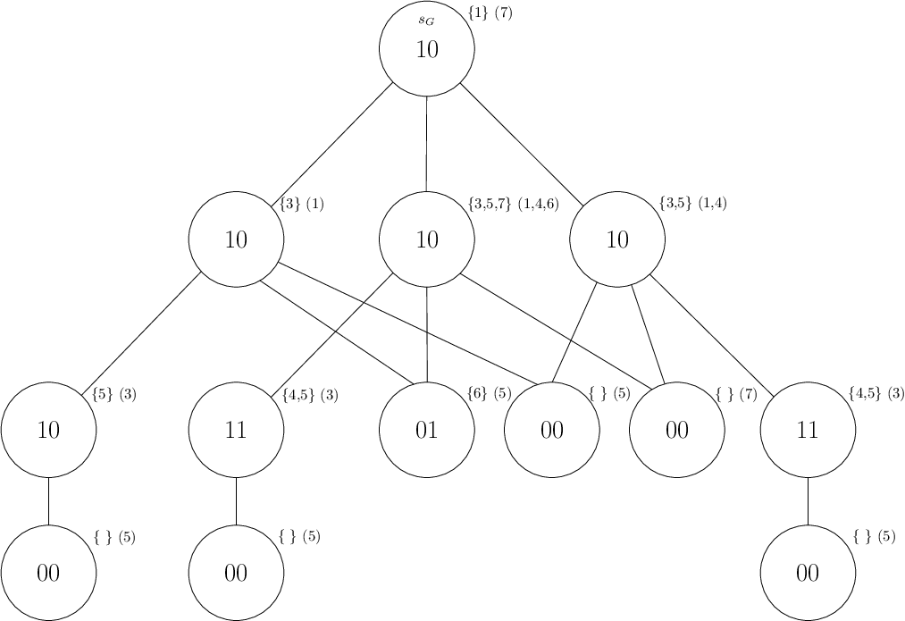
We now formally define the labeling scheme and prove the correctness of . We rely heavily on five carefully chosen sequences of node sets. The following notation will be used in the construction of these sequences and throughout the remainder of this section.
A set of nodes dominates a set of nodes if, for each node , there is a node that is adjacent to . For any set of nodes , denote by the neighbourhood of , i.e., .
2.1 Sequence Constructions and Properties
We construct five sequences of sets, indexed by . At a high level, will be the nodes that are informed before round , will be the nodes that are not informed before round , will be the uninformed nodes that are adjacent to at least one informed node in round , will be the nodes that are newly-informed in round , and will be the nodes that inform the nodes in in round . Recalling that denotes the source node of , we initialize the construction by setting . Our construction proceeds in stages, where stage is as follows:
- 1.
Define .
- 2.
Define .
- 3.
Define .
- 4.
Define to be a minimal subset of that dominates all nodes in .
- 5.
Define to be the subset of nodes in that are adjacent to exactly one node in .
The construction ends when . We now provide some useful facts about the sequences. The first two observations are direct consequences of the construction.
Fact 2.1.
for all .
Fact 2.2.
and .
Lemma 2.3.
For , we have .
Proof.
The following result can be viewed as a guarantee of progress in each stage: if there are any remaining uninformed nodes at stage , then at least one node will be newly informed in stage .
Lemma 2.4.
For each , if , then .
Proof.
If , then . So assume that . Since the graph is connected and is the disjoint union of and , it follows that .
Consider any . If each node that is adjacent to is also adjacent to at least one other node in , then also dominates all nodes in , contradicting the minimality of . Thus, there is at least one node that is adjacent to and not adjacent to any other node in . Hence, by definition, . ∎
The following result shows that the is well-defined.
Lemma 2.5.
For all , there exists a subset of that dominates all nodes in .
Proof.
Consider any node and suppose that does not have a neighbour in . By definition, dominates all nodes in , so it follows that . By Fact 2.1, , and by construction, , so . By the definition of , it follows that . But, implies that . It follows that has a neighbour in . Therefore, we have shown that every node has at least one neighbour in , which implies the desired result. ∎
Let be the smallest value of such that . We now give an upper bound on the value of .
Lemma 2.6.
.
Proof.
It follows from Lemmas 2.3 and 2.6 that every node in is contained in exactly one of the sets. We will later use this to ensure that all nodes in are eventually informed.
Corollary 2.7.
The sets form a partition of .
2.2 The Labeling Scheme
Formally, our labeling scheme assigns a label to each node in as follows:
- •
For each node , if there exists such that , then set at node . Otherwise, set at node .
- •
For each , for each node , arbitrarily pick one node that is adjacent to , and set at node . At all other nodes, set .
2.3 Correctness of algorithm
Our approach to showing that all nodes are eventually informed is to fully characterize which nodes transmit and which nodes are newly-informed in each round of the broadcast algorithm. Roughly speaking, we will show that, in an odd round , the nodes in transmit and all nodes in receive the source message for the first time. Then, in round , a certain subset of transmits, which results in the nodes of receiving “stay”. This will prompt the nodes of to transmit in round , which informs all nodes in . In this way, we will show that, for all , all nodes in are informed in round . Since we have already shown that the sets partition , this will show that broadcast is completed.
Lemma 2.8.
For each ,
- 1.
If , the following hold:
- (a)
Node transmits in round if and only if .
- (b)
Node receives for the first time in round if and only if .
- (a)
- 2.
If , the following holds:
- (a)
Node transmits “stay” in round if and only if and ’s label has .
- (a)
Proof.
The proof proceeds by induction on . In the base case, , we see that the source is the only node that transmits in round 1, it transmits , and the set of nodes that receive for the first time in round 1 is . Since and , this proves the base case.
For a fixed , assume that the result holds for all rounds . The induction step has two cases:
- •
for some .
First, consider a node such that ’s label has . By the induction hypothesis, receives for the first time in round . By the definition of the broadcast algorithm, transmits “stay” in round at line 19.
Conversely, suppose that transmits “stay” in round . By the algorithm, must have transmitted “stay” at line 19. From the code, it follows that ’s label has and received for the first time in round . By the induction hypothesis, . This completes the proof of 2(a).
- •
for some .
- –
Proof of 1(a):
First, suppose that . By the definition of , we know that . If , then, by the induction hypothesis, received for the first time in round . By the definition of the labeling scheme, we know that ’s label has . Hence, by lines 13-15, transmits in round . So, suppose . By the induction hypothesis, transmitted in round . By the definition of the labeling scheme, there is exactly one node in that is adjacent to and is labeled with . Therefore, exactly one neighbour of transmits “stay” in round , so receives “stay” in round . Hence, from lines 21-22, transmits in round .
Conversely, suppose that transmits in round . There are two cases to consider, depending on whether ’s transmission of in round occurred at line 15 or 22. In the first case, by line 15, we know that ’s label has , so, by the definition of labeling scheme, for some minimal . Since , the minimality of implies that . Further, by line 13, received for the first time in round . Hence, by the induction hypothesis, . By Lemma 2.3, it follows that . Thus, . Now, assume that ’s transmission occurred at line 22. By line 21, we know that received “stay” in round . By the induction hypothesis, the nodes in with are the nodes that transmit “stay” in round . It follows that is adjacent to exactly one node whose label has . By the definition of the labeling scheme, is adjacent to a node . By the induction hypothesis, since , we know that transmitted in round . By line 21, transmitted in round . Since , the induction hypothesis implies that received a message in round . Thus, .
- –
Proof of 1(b):
First, suppose that receives for the first time in round . Since receives in round , it must be adjacent to exactly one node that transmits in round . By 1(a), we know that is the set of nodes that transmit in round , which implies that is adjacent to exactly one node in . By the definition of , it follows that .
Conversely, suppose that . Then, by definition, is adjacent to exactly one node in . By 1(a), is the set of nodes that transmit in round . It follows that receives message in round . If received for the first time in some round , then, by the induction hypothesis, is contained in some where . This is impossible, by Lemma 2.3. Hence, received for the first time in round .
- –
∎
We now prove that our algorithm ensures that all nodes in are informed within rounds.
Theorem 2.9.
Consider any -node unlabeled graph with a designated source node with source message . By applying the 2-bit labeling scheme and then executing algorithm , all nodes in are informed within rounds.
3 Acknowledged Broadcast
To solve acknowledged broadcast, we provide an algorithm in which the source node receives an “ack” message in some round after all nodes in have received . At a high level, is obtained from by considering a particular node that receives last when is executed on . An additional bit in each node’s label is used to identify . Once it receives , node initiates the acknowledgement process by immediately transmitting an “ack” message that contains the round number in which it first received . The (unique) neighbour of that transmitted in round will receive this message, and it immediately transmits an “ack” message that contains the round number in which it first received . This process continues until the source node receives an “ack” message. The difficulty is that each node must know the round number in which it received , and the round numbers in which it transmits. This is implemented as follows. The source node appends “1” to its first transmitted message. Every other node determines the round number by recording the number that is appended to the first received message containing , and appends the round number (appropriately increased) whenever it transmits. The formal description of our acknowledged broadcast algorithm with source message is provided in Algorithm 2. We assume that there is a special “ack” message that is distinct from the source message and the “stay” message.
3.1 The Labeling Scheme
The labeling scheme is identical to except that one node will have a new label. This can be represented using an additional bit, , which is 1 for and 0 for all other nodes. The node is chosen as follows: label using labeling scheme and execute on the resulting labeled graph, then determine the first round after which there are no uninformed nodes, and choose to be a node that receives in round . If there is more than one such node, choose arbitrarily from among them.
We note that the labeling scheme will never assign certain labels to any node, which means we may safely use these labels in later schemes that are built on top of . At a high level, this is because is the only node with bit set to 1, and, as there are no remaining uninformed nodes after receives , our labeling scheme will set ’s bits and to 0 to indicate that should not transmit after receiving .
Fact 3.1.
For any graph , when the labeling scheme is applied to , no node is labeled with 101 or 111 or 011.
Proof.
By definition, node is the only node that has bit , so it is sufficient to prove that node has bit . By the definition of in Section 2.2, it is sufficient to prove that there is no value of such that . To obtain a contradiction, assume that there exists an such that , and let be the smallest such . Then, by the definition of , the fact that implies that . By the choice of by and Lemma 2.8, node receives for the first time in round , and there are no remaining uninformed nodes after this round. In particular, by Lemma 2.8, this means that for all , and so by Lemma 2.4. This implies that , so , which means , which contradicts the fact that . ∎
3.2 Correctness of algorithm
To prove the correctness of , we first observe that all transmissions of “ack” messages occur after all transmissions of and “stay” messages, i.e., the broadcast and the acknowledgement process do not interfere with one another. The first two observations follow from Lemma 2.8 and the fact that for all .
Observation 3.2.
The last round in which a node receives for the first time is .
Observation 3.3.
No transmissions of nor “stay” occur after round .
The next observation follows from Observation 3.2 and the definitions of algorithms and .
Observation 3.4.
The first transmission of “ack” occurs in round , and is transmitted by the unique node whose label has .
We now prove that the correct round number is appended to each message containing , which is necessary for the correctness of the acknowledgement process.
Lemma 3.5.
The messages and are transmitted only in round .
Proof.
The proof is by induction on . For the base case, , we see that the source node sends in its first transmission, and no other nodes transmit before receiving for the first time. As induction hypothesis, assume that, for all , a message or is only transmitted in round .
First, suppose that a node transmits a message . This occurs at line 26, which, by line 21, implies that received for the first time in round via some message . By the induction hypothesis, . Therefore, sets informedRound equal to at line 12. So, when transmits , it follows that , as desired.
Next, suppose that a node transmits a message . If this transmission occurs at line 18, then, by line 16, we know that received for the first time in round via some message . By the induction hypothesis, . Therefore, sets informedRound equal to at line 12. So, when transmits , it follows that , as desired. The other possibility is that the transmission by occurs at line 30, which, by line 28, implies that received a message in round . By the induction hypothesis, . So, when transmits , it follows that , as desired. ∎
From Lemma 3.5, it follows that if a node first receives in round , then the informedRound variable at node is equal to in all subsequent rounds. Similarly, if a node transmits a message containing in round , then the transmitRounds variable at node contains in all subsequent rounds.
We complete the proof of correctness of by showing that the source node will eventually receive an “ack” message. First, we show that at most one node transmits “ack” in any round, which implies that no collisions occur during the acknowledgement procedure.
Lemma 3.6.
After round , at most one node transmits in each round.
Proof.
The proof is by induction on the round number . For the base case, Observations 3.2-3.4 imply that the unique node with in its label transmits in round . As induction hypothesis, assume that at most one node transmits in round . If no node transmits in round , then, from Observation 3.3 and the code, no node transmits in round . Otherwise, suppose that exactly one node transmits in round . By Observation 3.3, this message is of the form . At most one neighbour of contains in its transmitRounds variable since received in round . From Observation 3.3 and the code, no other node transmits in round . ∎
We now show that the “ack” message propagates through a sequence of nodes, where each node is contained in some . Further, the indices of the corresponding sets form a decreasing sequence, which implies that will eventually receive an “ack” message.
Lemma 3.7.
For each , in round , some node in with receives .
Proof.
The proof is by induction on . For the base case , Observations 3.2 and 3.4 imply that transmits an message in round . By Lemma 3.6, no other node transmits in round , so all of ’s neighbours receive the transmitted “ack” message. Since received in round , it follows that a neighbour of transmitted in round . By Lemma 2.8, . Therefore, the statement is satisfied with , which completes the base case.
As induction hypothesis, assume that, for some , in round , some node with receives . Since , Lemma 2.8 implies that transmitted in round . Therefore, its transmitRounds variable contains . By lines 33-35 of , it follows that transmits in round . We note that the value of informedRound at must be less than , since must have received for the first time before it transmitted in round . From Lemma 2.8, we conclude that for some . So we have shown that transmits for some in round . By Lemma 3.6, no other node transmits in round , so all of ’s neighbours receive the transmitted “ack” message in round . Since received in round , it follows that a neighbour of transmitted in round . By Lemma 2.8, . To summarize, we have shown that in round , some node with receives , which completes the induction. ∎
Corollary 3.8.
There exists a round in which the source node receives an “ack” message.
The correctness of follows directly from Corollary 3.8, which gives us the main result of this section.
Theorem 3.9.
Consider any -node unlabeled graph with a designated source node with source message . By applying the 3-bit labeling scheme and then executing algorithm , all nodes in are informed by round , and receives an “ack” message by round .
Finally, we note that and can be used to ensure that there is a common round in which all nodes know that the broadcast of the source’s message has been completed. First, run , and have the source node record the round number in which it first receives an “ack” message. Then, the source executes with message . All nodes will receive the value of before round . So, in round , all nodes know that the original broadcast of has been completed.
4 Broadcast from an Arbitrary Source
In this section, we consider the more difficult scenario in which the source node is not designated in when the labeling scheme is applied. We provide a labeling scheme of length 3 and a universal deterministic algorithm that solves (acknowledged) broadcast regardless of which node initially knows the source message.
4.1 The Labeling Scheme
Choose an arbitrary node and label this node using the string 111. Apply the labeling scheme to the remaining nodes in the network, but use as the source node (as there is no designated source ). By Fact 3.1, note that does not assign the label 111 to any node, so the node is a unique node in the network that our algorithm can use to play a special role in coordinating the broadcast, regardless of which node is the actual source . Let be the node labeled 001 by , i.e., the node that initiates the acknowledgement process in an execution of .
4.2 Algorithm
- 1.
Perform an acknowledged broadcast using with node as source and with message “initialize”. Each node stores in a variable the timestamp value contained in the first “initialize” message it received. In particular, node sets to 0. When starting the acknowledgement process, node appends to the “ack” message the timestamp value . This step of the algorithm ends when receives the “ack” message, at which point it knows the value of and it knows that all nodes have received “initialize”.
- 2.
Perform an acknowledged broadcast using a modified version of with node as the source and with message (“ready”,). The modification to the algorithm is that the node does not initiate the acknowledgement process. Instead, when the source node receives the “ready” message, it waits rounds, then initiates the acknowledgement process (as described in ), but with the source message appended to the “ack” message. (Waiting rounds ensures that this acknowledgement process started by does not begin until the “ready” broadcast has completed.) This step of the algorithm ends when receives the “ack” message, at which point it knows the source message . Further, all nodes know the value of .
- 3.
Perform a broadcast using with node as source and with message . At the end of this broadcast, all nodes know the source message . If each node waits rounds after receiving in this step, then the algorithm solves acknowledged broadcast, as all nodes can be sure that all nodes have received .
5 Conclusion
We presented a universal deterministic broadcast algorithm using labeling schemes of constant length that works for arbitrary radio networks. Our schemes are of length 2, and we showed how to solved acknowledged broadcast with schemes of length 3 (but only 5 different labels). In the case where the source node is not designated when the labeling scheme is applied, our scheme also has length 3, but uses 6 different labels. It would be interesting to determine if schemes using fewer than 4 different labels are sufficient for broadcast. We do not have any impossibility results beyond the trivial 1-bit lower bound (2 different labels), and we are intrigued by the possibility that there exists a scheme of length 1 for broadcast. A positive answer can be obtained for broadcast in graphs where each node’s distance to the source is at most 2: use and from Section 2, but use only the bit , and modify the definitions of and by changing instances of to . We can also show that it is possible to perform broadcast in series-parallel graphs and grid graphs using single-bit labels. In both cases, using the same technique from Section 3, acknowledged broadcast is possible using 3 labels. It would also be interesting to determine whether or not acknowledged broadcast is possible in all graphs using 1-bit labels, and, if not, if it is possible using 2-bit labels. Another open question is whether acknowledged broadcast can be performed with only constant-length messages, instead of bits. The above open questions can also be asked for the case where the source node is not designated when the labeling scheme is applied.
In this paper, we focused on the feasibility of radio broadcast with short labels, and we did not try to optimize the time complexity. Our algorithm works in time . This yields the following open problem. What is the fastest universal deterministic broadcast algorithm using labeling schemes of constant length?
References
- [1] Serge Abiteboul, Stephen Alstrup, Haim Kaplan, Tova Milo, and Theis Rauhe. Compact labeling scheme for ancestor queries. SIAM J. Comput., 35(6):1295–1309, 2006.
- [2] Noga Alon, Amotz Bar-Noy, Nathan Linial, and David Peleg. A lower bound for radio broadcast. J. Comput. Syst. Sci., 43(2):290–298, 1991.
- [3] Reuven Bar-Yehuda, Oded Goldreich, and Alon Itai. On the time-complexity of broadcast in multi-hop radio networks: An exponential gap between determinism and randomization. J. Comput. Syst. Sci., 45(1):104–126, 1992.
- [4] Danilo Bruschi and Massimiliano Del Pinto. Lower bounds for the broadcast problem in mobile radio networks. Distributed Computing, 10(3):129–135, 1997.
- [5] Imrich Chlamtac and Shay Kutten. On broadcasting in radio networks-problem analysis and protocol design. IEEE Trans. Communications, 33(12):1240–1246, 1985.
- [6] Imrich Chlamtac and O. Weinstein. Distributed ”wave” broadcasting in mobil multi-hop radio networks. In Proceedings of the 7th International Conference on Distributed Computing Systems, Berlin, Germany, September 1987, pages 82–89. IEEE Computer Society, 1987.
- [7] Bogdan S. Chlebus, Leszek Gasieniec, Alan Gibbons, Andrzej Pelc, and Wojciech Rytter. Deterministic broadcasting in ad hoc radio networks. Distributed Computing, 15(1):27–38, 2002.
- [8] Bogdan S. Chlebus, Leszek Gasieniec, Anna Östlin, and John Michael Robson. Deterministic radio broadcasting. In Ugo Montanari, José D. P. Rolim, and Emo Welzl, editors, Automata, Languages and Programming, 27th International Colloquium, ICALP 2000, Geneva, Switzerland, July 9-15, 2000, Proceedings, volume 1853 of Lecture Notes in Computer Science, pages 717–728. Springer, 2000.
- [9] Marek Chrobak, Leszek Gasieniec, and Wojciech Rytter. Fast broadcasting and gossiping in radio networks. J. Algorithms, 43(2):177–189, 2002.
- [10] Andrea E. F. Clementi, Angelo Monti, and Riccardo Silvestri. Distributed broadcast in radio networks of unknown topology. Theor. Comput. Sci., 302(1-3):337–364, 2003.
- [11] Reuven Cohen, Pierre Fraigniaud, David Ilcinkas, Amos Korman, and David Peleg. Label-guided graph exploration by a finite automaton. ACM Trans. Algorithms, 4(4):42:1–42:18, 2008.
- [12] Artur Czumaj and Peter Davies. Faster deterministic communication in radio networks. In Ioannis Chatzigiannakis, Michael Mitzenmacher, Yuval Rabani, and Davide Sangiorgi, editors, 43rd International Colloquium on Automata, Languages, and Programming, ICALP 2016, July 11-15, 2016, Rome, Italy, volume 55 of LIPIcs, pages 139:1–139:14. Schloss Dagstuhl - Leibniz-Zentrum fuer Informatik, 2016.
- [13] Artur Czumaj and Wojciech Rytter. Broadcasting algorithms in radio networks with unknown topology. J. Algorithms, 60(2):115–143, 2006.
- [14] Dariusz Dereniowski and Andrzej Pelc. Drawing maps with advice. J. Parallel Distrib. Comput., 72(2):132–143, 2012.
- [15] Michael Elkin and Guy Kortsarz. An improved algorithm for radio broadcast. ACM Trans. Algorithms, 3(1):8:1–8:21, 2007.
- [16] Yuval Emek, Pierre Fraigniaud, Amos Korman, and Adi Rosén. Online computation with advice. Theor. Comput. Sci., 412(24):2642–2656, 2011.
- [17] Pierre Fraigniaud, Cyril Gavoille, David Ilcinkas, and Andrzej Pelc. Distributed computing with advice: information sensitivity of graph coloring. Distributed Computing, 21(6):395–403, 2009.
- [18] Pierre Fraigniaud, David Ilcinkas, and Andrzej Pelc. Tree exploration with advice. Inf. Comput., 206(11):1276–1287, 2008.
- [19] Pierre Fraigniaud, David Ilcinkas, and Andrzej Pelc. Communication algorithms with advice. J. Comput. Syst. Sci., 76(3-4):222–232, 2010.
- [20] Pierre Fraigniaud, Amos Korman, and Emmanuelle Lebhar. Local MST computation with short advice. Theory Comput. Syst., 47(4):920–933, 2010.
- [21] Emanuele G. Fusco, Andrzej Pelc, and Rossella Petreschi. Topology recognition with advice. Inf. Comput., 247:254–265, 2016.
- [22] Iris Gaber and Yishay Mansour. Centralized broadcast in multihop radio networks. J. Algorithms, 46(1):1–20, 2003.
- [23] Leszek Gasieniec, Aris Pagourtzis, Igor Potapov, and Tomasz Radzik. Deterministic communication in radio networks with large labels. Algorithmica, 47(1):97–117, 2007.
- [24] Leszek Gasieniec, David Peleg, and Qin Xin. Faster communication in known topology radio networks. Distributed Computing, 19(4):289–300, 2007.
- [25] Leszek Gasieniec, Igor Potapov, and Qin Xin. Time efficient centralized gossiping in radio networks. Theor. Comput. Sci., 383(1):45–58, 2007.
- [26] Cyril Gavoille, David Peleg, Stéphane Pérennes, and Ran Raz. Distance labeling in graphs. J. Algorithms, 53(1):85–112, 2004.
- [27] Christian Glacet, Avery Miller, and Andrzej Pelc. Time vs. information tradeoffs for leader election in anonymous trees. ACM Trans. Algorithms, 13(3):31:1–31:41, 2017.
- [28] Barun Gorain and Andrzej Pelc. Short labeling schemes for topology recognition in wireless tree networks. In Shantanu Das and Sébastien Tixeuil, editors, Structural Information and Communication Complexity - 24th International Colloquium, SIROCCO 2017, Porquerolles, France, June 19-22, 2017, Revised Selected Papers, volume 10641 of Lecture Notes in Computer Science, pages 37–52. Springer, 2017.
- [29] Barun Gorain and Andrzej Pelc. Finding the size of a radio network with short labels. In Paolo Bellavista and Vijay K. Garg, editors, Proceedings of the 19th International Conference on Distributed Computing and Networking, ICDCN 2018, Varanasi, India, January 4-7, 2018, pages 10:1–10:10. ACM, 2018.
- [30] David Ilcinkas, Dariusz R. Kowalski, and Andrzej Pelc. Fast radio broadcasting with advice. Theor. Comput. Sci., 411(14-15):1544–1557, 2010.
- [31] Michal Katz, Nir A. Katz, Amos Korman, and David Peleg. Labeling schemes for flow and connectivity. SIAM J. Comput., 34(1):23–40, 2004.
- [32] Amos Korman, Shay Kutten, and David Peleg. Proof labeling schemes. Distributed Computing, 22(4):215–233, 2010.
- [33] Dariusz R. Kowalski and Andrzej Pelc. Broadcasting in undirected ad hoc radio networks. Distributed Computing, 18(1):43–57, 2005.
- [34] Dariusz R. Kowalski and Andrzej Pelc. Time complexity of radio broadcasting: adaptiveness vs. obliviousness and randomization vs. determinism. Theor. Comput. Sci., 333(3):355–371, 2005.
- [35] Dariusz R. Kowalski and Andrzej Pelc. Optimal deterministic broadcasting in known topology radio networks. Distributed Computing, 19(3):185–195, 2007.
- [36] Dariusz R. Kowalski and Andrzej Pelc. Leader election in ad hoc radio networks: A keen ear helps. J. Comput. Syst. Sci., 79(7):1164–1180, 2013.
- [37] Eyal Kushilevitz and Yishay Mansour. An omega(D log (N/D)) lower bound for broadcast in radio networks. SIAM J. Comput., 27(3):702–712, 1998.
- [38] Nicolas Nisse and David Soguet. Graph searching with advice. Theor. Comput. Sci., 410(14):1307–1318, 2009.