Primordial black hole formation by vacuum bubbles
Abstract
Vacuum bubbles may nucleate during the inflationary epoch and expand, reaching relativistic speeds. After inflation ends, the bubbles are quickly slowed down, transferring their momentum to a shock wave that propagates outwards in the radiation background. The ultimate fate of the bubble depends on its size. Bubbles smaller than certain critical size collapse to ordinary black holes, while in the supercritical case the bubble interior inflates, forming a baby universe, which is connected to the exterior region by a wormhole. The wormhole then closes up, turning into two black holes at its two mouths. We use numerical simulations to find the masses of black holes formed in this scenario, both in subcritical and supercritical regime. The resulting mass spectrum is extremely broad, ranging over many orders of magnitude. For some parameter values, these black holes can serve as seeds for supermassive black holes and may account for LIGO observations.
I Introduction
Primordial black holes (PBHs) are hypothetical black holes formed in the early universe before any nonlinear large scale structure and galaxies. The idea was conceived and developed decades ago [1, 2, 3], and since then PBHs have received considerable attention, despite the fact that their existence is yet to be supported by observations. Depending on the model, PBH masses can range from as low as the Planck mass ( g) to many orders of magnitude above the solar mass ( g). By contrast, black holes formed by stellar collapse cannot have mass smaller than . Small PBHs could be sources of Hawking radiation, whereas PBHs with have been suggested as a candidate for (at least part of) the cold dark matter and as possible seeds of supermassive black holes. Numerous mechanisms of PBH formation have been proposed over the years. In many scenarios (e.g., [4, 5, 6, 7, 8]), overdensity produced during inflation may overcome pressure and collapse into a black hole after it reenters the horizon during the radiation-dominated era. Other possibilities are related to first-order phase transitions [9, 10, 11], the collapse of cosmic string loops [12, 13, 14] and domain walls [14, 15, 16, 17], etc.
In this paper, we shall use numerical simulations to explore the possibility, recently suggested in [16], that PBH could be formed by nonperturbative quantum effects in the early universe. Specifically, we will show that spontaneous nucleation of vacuum bubbles during the inflationary epoch can result in black holes with a wide mass spectrum at the present time.
The physical mechanism responsible for this phenomenon is easy to understand. The inflationary expansion of the universe is driven by the high energy density of the false vacuum 11 1 We use the term "false vacuum" somewhat loosely, including a slowly rolling inflaton in this category.. Bubble nucleation may occur by quantum tunneling if the underlying physics includes some vacuum states, other than our present vacuum, with energy density (we will be interested in the case where ). A two-dimensional energy landscape corresponding to this setup is illustrated in Fig. 1. The inflaton field slowly "rolls" along the gentle slope in the landscape towards a local energy density minimum representing our vacuum. As it rolls, it can tunnel through a potential barrier to another vacuum of energy density higher than ours. The tunneling occurs through bubble nucleation: a small spherical bubble of the new vacuum spontaneously forms in the inflating background [18]. Once the bubble nucleates, it expands with acceleration, acquiring a large Lorentz factor. This growth of the bubble is caused by the large vacuum tension outside (which is greater than the vacuum tension inside). At the end of inflation, the false vacuum outside the bubble decays into hot radiation. The bubble wall runs into the radiation and quickly loses much of its energy, producing a shock wave that propagates outwards. A black hole is then formed by one of the two different scenarios, depending on the size of the bubble. (i) The bubble wall is pulled inwards by the interior vacuum tension, the wall tension, as well as the radiation pressure; so it shrinks and eventually collapses to a singularity. Following [16], we shall refer to such bubbles as subcritical. (ii) If in the course of bubble expansion its size exceeds the interior de Sitter horizon, the bubble begins to inflate. In the latter case, the bubble continues to expand without bound and a wormhole is created outside the bubble wall, connecting the inflating baby universe inside and the FRW parent universe dominated by radiation. Such bubbles will be called supercritical.

It was argued in Ref. [16] that the bubble transfers most of its kinetic energy to surrounding matter and comes to rest with respect to the Hubble flow on a time scale much shorter than the Hubble time. If the exterior region were filled with pressureless dust, an empty layer would form around the bubble, so the bubble would be completely isolated from matter. In this case the bubble evolution and the mass of the resulting black hole can be found analytically. The case with a radiation background is more involved, due to the pressure exerted on the wall. Also, if a wormhole is formed, some radiation may follow the bubble into the wormhole. Both of these effects may influence the black hole mass.
Our goal in this paper is to numerically study black hole formation by vacuum bubbles and to determine the resulting spectrum of black hole masses. The paper is organized as follows. In Section II we discuss the bubble dynamics in more detail and review some relevant earlier work. Our simulation model is described in Section III, and simulation results are presented in Section IV. We calculate the black hole mass spectrum in Section V and discuss observational implications and constraints on the model parameters in Section VI. Our conclusions are summarized and discussed in Section VII. We set throughout the paper.
II Bubble dynamics
We consider an idealized model where inflation ends instantaneously at time , so that false vacuum outside the bubble is instantly turned into radiation of initial energy density . We also assume, as in Ref. [16], that particles are reflected from the bubble wall, so radiation cannot penetrate the bubble and the bubble interior always remains pure de Sitter.
As we mentioned in the Introduction, the bubble evolution can lead to two possible outcomes, depending on the bubble size. We first consider subcritical bubbles.
II.1 Subcritical bubbles
When the bubble transfers its momentum to radiation and comes to rest with respect to the Hubble flow at , it continues to expand by inertia. But the forces due to the tension of the vacuum inside the bubble and due to the tension of the bubble wall are both directed inwards, so the bubble wall accelerates inwards, away from the surrounding radiation, and we can expect that in a few Hubble times the interaction of the bubble with radiation becomes negligible.

In the subcritical case, the bubble eventually stops expanding and collapses to a Schwarzschild singularity; the corresponding conformal diagram is shown in Fig. 2. We can estimate the mass of the resulting black hole by assuming that the interaction with radiation is negligible right after the initial momentum transfer at . Then the bubble dynamics is the same as it would be if the exterior region were asymptotically Minkowski. In this case the bubble can be characterized by a conserved mass parameter given by [19]
| (1) |
where is the bubble radius and the overdot stands for a derivative with respect to the proper time on the bubble wall. We have also defined22 2 is the rate of inflation in a vacuum of energy density , and is the rate at which an isolated domain wall of tension would inflate due to its self-gravity.
| (2) |
and
| (3) |
where is the bubble wall tension. The first term in Eq. (1) is the interior vacuum energy of the bubble, the second term is the energy of the expanding wall, and the last term the gravitational self-energy of the wall.
Since , it can be evaluated at , when with the Hubble constant during inflation and the bubble radius at . The black hole mass is then simply . Assuming that the bubble is much bigger than the horizon, , this is given by
| (4) |
The maximal radius of expansion of the bubble can be found by setting in Eq. (1) and solving for . A solution exists only if is smaller than certain critical mass . An exact expression for was found in Ref. [20]; it is rather cumbersome and we will not reproduce it here. By order of magnitude, can be estimated as [16]
| (5) |
On dimensional grounds, and , where and are the energy scales of the interior vacuum and of the bubble wall, respectively. Then, with , we have and . In this case the maximum expansion radius is related to the black hole mass as . As is increased, grows and reaches its largest value, at the critical mass. On the other hand, a situation where is also possible; then and . The choice of parameters in our simulations was dictated mostly by the computing constraints.
We do not expect the estimates (1) and (4) to be very accurate. Radiation does work on the bubble while it expands (which decreases the bubble mass) and while it contracts (which increases the bubble mass). Since the radiation density is higher during the expanding phase, one can expect the overall effect to be mass reduction (except in cases where the expanding phase is very short). But since the contact with radiation effectively ceases within a few Hubble times, it was suggested in [16] that Eqs. (1) and (4) should give the right order of magnitude. We shall see that this is indeed the case.
II.2 Supercritical bubbles
For , the bubble expands to a radius greater than , and the bubble interior begins to inflate. At this point nothing can stop it from growing33 3 For , the bubble wall starts inflating, due to its repulsive gravity, when its radius exceeds . Inflation in the bubble interior begins when the wall expands to .. In this “supercritical” case, the bubble grows into a baby universe, which is connected to the parent universe outside by a wormhole throat. The wormhole closes up on a timescale , and black holes of mass are formed at its two mouths. From then on, the baby universe has no impact on further evolution of the exterior FRW region. The corresponding spacetime structure was discussed in Ref. [16]; it is illustrated in the conformal diagram in Fig. 3. As emphasized in [16], wormhole formation in this spacetime does not violate any singularity theorems and does not require violation of the null energy condition.
An unusual feature of the diagram in Fig. 3 is the presence of a white hole region (marked WH), as in the Kruskal spacetime of an eternal black hole. The boundaries of black and white holes are usually defined by their event horizons, and we adopted this convention in the figure. A more physically motivated definition is to use apparent (or trapping) horizons (see e.g. Ref. [24] and references therein). We followed this approach in our simulations; see Sec. III.D for more detail.

The shock wave produced by the bubble wall propagates outwards at the speed of sound; its trajectory is shown by a dashed curve in the diagram. The region outside the shock remains unperturbed and is described by the FRW solution. On the other hand, the evolution inside the shock radius can be rather complicated. In particular, some radiation flows out of the white hole region, resulting in a decrease of the black hole mass. This can be thought of as an inverse process of radiation flowing into a black hole, which would increase the mass.
A related problem has been studied in Ref. [17], which investigated the collapse of spherical domain walls formed during inflation. In this case, inflation ends both inside and outside the wall. If the wall expands to a radius greater than , it starts inflating and a radiation-filled baby universe is formed. It was pointed out in [17] that the Schwarzschild radius of the resulting black hole cannot exceed the radius of the comoving FRW region affected by the wall when it comes within the cosmological horizon. The affected region is marked by the rarefaction wave that propagates away from the wall at the speed of sound. The resulting bound on the black hole mass is
| (6) |
The situation in our case is very similar, except the affected region is now bounded by the shock front. Hence we expect the same bound to apply. Numerical simulations in Ref. [17] showed that black hole masses in supercritical regime are , so the bound (6) is nearly saturated. Here, we shall see that the same conclusion applies to supercritical bubbles with a sufficiently large .
III Simulation setup
In this section we consider the equations of motion as well as the initial and boundary conditions necessary for numerical simulations of a vacuum bubble embedded in an otherwise homogeneous radiation-dominated universe. We also indicate how we read the black hole mass from the simulation results and discuss some simulation issues.
III.1 Equations of motion and gauge conditions
The spacetime is assumed to be spherically symmetric, and the metric we use for the exterior region (outside of the bubble) is
| (7) |
where and are functions of the coordinates and . The radiation fluid is generally described by its energy density , pressure with , and 4-velocity with .
To fix the gauge, we choose the coordinates comoving with the fluid, in which and . In this gauge, both the equations of motion and the boundary conditions take a particularly simple form. Since the fluid is confined to the bubble exterior, the normal component of the fluid velocity vanishes at the bubble wall. The tangential velocity vanishes by symmetry. It follows that the wall is comoving with the fluid; hence it remains at a fixed value of the comoving radius, . With a different choice of gauge we would have to impose boundary conditions on a moving boundary, which is considerably more complicated.
Following Ref. [21] we introduce
| (8) |
where and . Our goal is to solve Einstein’s equations in order to find and . By the following transformations
| (9) |
all variables become dimensionless. In this section we use these new variables and drop the tilde. For instance, the time at the end of inflation now becomes . To restore the physical value of a certain quantity, one simply needs to multiply by an appropriate conversion factor. For example, the conversion factor for mass is .
Einstein’s equations then take the form
| (10) |
| (11) |
| (12) |
| (13) |
| (14) |
| (15) |
where
| (16) |
is the Misner-Sharp mass parameter [22] that we shall use to characterize the mass of the central object.
Eqs. (14) and (15) can be written in an equivalent form:
| (17) |
| (18) |
We used different equations in different situations in order to avoid a vanishing denominator. For instance, in the subcritical case, the bubble grows and then shrinks, so the value of at the wall goes from positive to negative at the turning point. Hence we use Eqs. (14) and (15) to evolve and respectively, since must not appear in the denominator. Similarly, in the supercritical case, crosses zero when the wormhole throat is formed, so we use Eqs. (17) and (18).
The gauge condition leaves the freedom of time transformations, . We can fix the gauge completely by specifying on any timelike curve. Before the bubble is removed for reasons discussed below (Subsection IV.B), a convenient choice is to set at the bubble wall. Then our time coordinate coincides with the proper time at the wall.
III.2 Boundary conditions
We first comment on the number of boundary conditions required for our problem. The following argument was suggested to us by Andrei Gruzinov.
Introducing two new variables, and , instead of and , the equations of motion (11)-(15) can be represented as
| (19) |
| (20) |
| (21) |
where "…" means terms without derivatives and we have used Eq. (10) to express in terms of in (20). Now, Eqs. (19) do not require boundary conditions (only initial conditions) and Eqs. (20) and (21) represent a wave with a (high-frequency) sound speed . We thus have one propagating degree of freedom, which requires one left and one right boundary condition.
Variables outside of the shock front should be described by the unperturbed FRW solution, so the outer boundary condition is easy to impose. Before the bubble is removed, the wall serves as the inner boundary. The bubble interior is described by de Sitter space with energy density . The boundary conditions at the wall can be obtained using Israel’s junction conditions. This is done in Appendix A.44 4 The equation of motion of the wall is also derived in Appendix A, but we did not use it in our simulations. As we discussed, we only need one boundary condition at ; we use the condition (69):
| (22) |
We also set on the inner boundary at all times, even after the bubble wall is removed.
III.3 Initial conditions
We assume an idealized initial state where inflation ends instantaneously at and false vacuum energy immediately turns into radiation of uniform energy density
| (23) |
Since the lapse function at , it follows from Eq. (10) that in the entire region outside of the bubble. One might expect that at this whole region is described by the FRW solution. Then, with a suitable normalization of , we would have , , , and . However, these values cannot be imposed as initial conditions in the entire region .
At the initial moment, the bubble wall moving with a large Lorentz factor comes into contact with the radiation fluid that surrounds it. On the other hand, we are working in a gauge where the radiation is comoving with the wall at . Clearly, this condition cannot be satisfied if the FRW solution outside the bubble is unperturbed. We deal with this problem by modifying the FRW solution in a thin layer around the bubble.
The Misner-Sharp mass of the bubble at is , where we have assumed that . On the other hand, is also given by Eq. (1) with . Then by the definition of and , the initial value of at the wall is given by
| (24) |
To smooth out the discontinuity between this and the FRW value of , we use the following function for the initial profile of ,
| (25) |
where characterizes the thickness of the layer that connects the wall and the FRW universe.
To fix the remaining initial conditions, we assume the spatial metric . Then and it follows from the definition of that
| (26) |
can now be found by numerically integrating Eq. (26). To illustrate the deviation of our initial state from FRW, we plot the functions and in Fig. 4. (Both of these functions are equal to 1 in an FRW universe.)
The Misner-Sharp mass within a radius at can be found from the relation [23] , which gives . Then by the definition of , the initial profile of is
| (27) |


It can be shown [16] that in our gauge the initial value of at the wall is related to the initial Lorentz factor of the wall (relative to an FRW observer) by
| (28) |
In our simulations, we used and as free parameters. The value of can be determined from Eqs. (1), (8) and (28).
A profile of with a finite means that the fluid already acquired some kinetic energy at in a layer of width . It is shown in Ref. [16] that the wall loses most of its kinetic energy and comes to rest with respect to the radiation fluid within a time (a more accurate calculation gives ). This suggests that should be chosen so that . Indeed, we have verified that reducing below this value does not have a significant impact on the black hole mass.
III.4 Expansions and horizons
We determine the formation of a black hole by checking if an apparent horizon bounding a trapped region is formed. Let and be the expansions of outgoing and ingoing radial null geodesics respectively; then a surface is trapped if , and anti-trapped if . In our coordinate system [25],
| (29) |
The apparent horizon of a black hole is foliated by marginal spheres with and We also define the white hole (apparent) horizon and cosmological (apparent) horizon to be hypersurfaces foliated by marginal spheres with and A spherical surface is anti-trapped within the white hole horizon, and is normal (with and ) if it lies between the white (or black hole) and the cosmological horizon. The cosmological horizon and the Hubble radius coincide in a flat FRW universe.
III.5 Simulation issues
We use finite-difference method and Runge-Kutta integration to solve the PDEs.
Special attention is needed on the shock wave. The shock formed by the interaction of the fast-moving wall and the radiation may lead to numerical instability. A standard and convenient trick to handle this is to introduce artificial viscosity [27] in order to smooth out the discontinuity. Following [26], we add an extra term to ,
| (30) |
where is an adjustable coefficient that controls the viscosity strength, and is the grid size. When needed, we replace by
| (31) |
to avoid in the denominator in Eq. (30).
Additionally, in order to improve the efficiency of the code, we use an adaptive non-uniform mesh. At the beginning of the simulation, a sufficiently high resolution is used until a shock wave is formed. Then we reduce the mesh density in regions far away from the shock. We keep track of the shock and make sure there is a sufficient number of grid points there.
Another issue is related to the early evolution of the bubble wall. A very large initial Lorentz factor tends to break down the code before any desirable results are obtained. Throughout the simulations we used . This leads to a constraint on . The initial Lorentz factor can be estimated as [16] . Using this and Eqs. (4) and (5), it can be shown that the radii of subcritical bubbles must satisfy . On the other hand, we are mostly interested in bubbles of initial radius greater than the horizon, . This gives a rather limited range of values for . For supercritical bubbles, we are free to use a large value for , but are restricted by the simulation runtime.
IV Simulation results
IV.1 Shock propagation


The formation and propagation of the shock wave produced by the bubble are illustrated in Fig. 5. The figure shows the radiation density profile at successive moments of time. As the bubble wall hits the ambient radiation, a thin overdense layer is formed right outside the wall. In this example, the density in the layer exceeds that in the FRW region by more than 100 times. The overdense layer spreads and develops a sharp shock front, which then propagates outwards. Meanwhile, the radiation density next to the wall rapidly drops, and in less than a Hubble time becomes much smaller than that in the FRW region.
The density contrast across the shock , where , is very large immediately after the wall hits the ambient radiation, but rapidly drops and becomes in about a Hubble time. Fig. 6 shows the subsequent evolution of , which can be approximated as .
As the shock propagates outwards, the empty layer created by the bubble impact is gradually filled with radiation. In Fig. 7 we show the radiation density profile at several moments right before and after black hole formation, both for a subcritical and a supercritical bubble. In both cases, in a few Hubble times after the black hole is formed, it is surrounded by a nearly uniform radiation background.


IV.2 Black hole mass
IV.2.1 Subcritical bubble

The Misner-Sharp mass of the bubble decreases dramatically within a time scale due to momentum transfer to radiation. At later times, the mass continues to change due to the radiation pressure, but it approaches a constant after about one Hubble time (Fig. 8). In the subcritical case, the bubble radius reaches a maximum and then decreases. An apparent horizon is formed when at the wall. We regard this as a signal of black hole formation. The black hole mass can be estimated as the Misner-Sharp mass at the apparent horizon.
The black hole masses obtained from the simulations are compared with the analytic estimate (4) in Table. 1. We see that Eq. (4) gives a good estimate within a factor of 2. As expected, in most examples the actual black hole mass is lower than estimated, because of the radiation pressure during the expansion phase of the bubble. In some examples, however, the actual mass is slightly higher. This is because the expansion phase in these cases was very short.
At later times, the black hole mass grows by accretion of radiation, but the resulting mass increase is no more than by a factor of 2 [17].
| Parameters | |||
|---|---|---|---|
| , | 2 | 0.5 | 0.3 |
| 3 | 1.7 | 1.0 | |
| 4 | 3.9 | 2.1 | |
| 5 | 7.6 | 3.7 | |
| , | 2 | 0.8 | 0.7 |
| , | 1.8 | 0.8 | 0.9 |
| , | 1 | 0.3 | 0.3 |
IV.2.2 Supercritical bubble
In the supercritical case, a wormhole develops outside of the bubble wall, and the bubble starts to inflate. In Fig. 9 we show the area radius as a function of the comoving radius at several successive moments of time. We see that develops a minimum outside of the wall, signaling the formation of a wormhole. Since the bubble is rapidly expanding, the radius grows sharply towards the wall.
In order to simulate the evolution of the region near the bubble wall, high resolution is needed. However, since the bubble grows supersonically away from the exterior region and thus gets detached from the fluid, we cut off the wall as well as a layer immediately outside, so as to prevent from changing steeply near the inner boundary and avoid simulation breakdown. This excision does not affect the evolution of the exterior region.
The black hole formation is signaled by the horizon bifurcation point, where . (This is the point at the intersection of the two apparent horizon lines in the conformal diagram of Fig. 3.) At this point two black holes of equal mass are formed, one for the observer in the baby universe and the other in the exterior FRW universe.
The two black holes start with identical masses, but the masses can grow later by accretion and do not have to remain equal. The mass accretion on the exterior black hole has been studied in Ref. [17] in the domain wall scenario, with the conclusion that it increases the black hole mass by approximately a factor of 2. For a large supercritical bubble, the perturbation caused by the shock should mostly dissipate by the time of black hole formation, and we expect that the accretion process will be very similar to the domain wall case, with similar result.
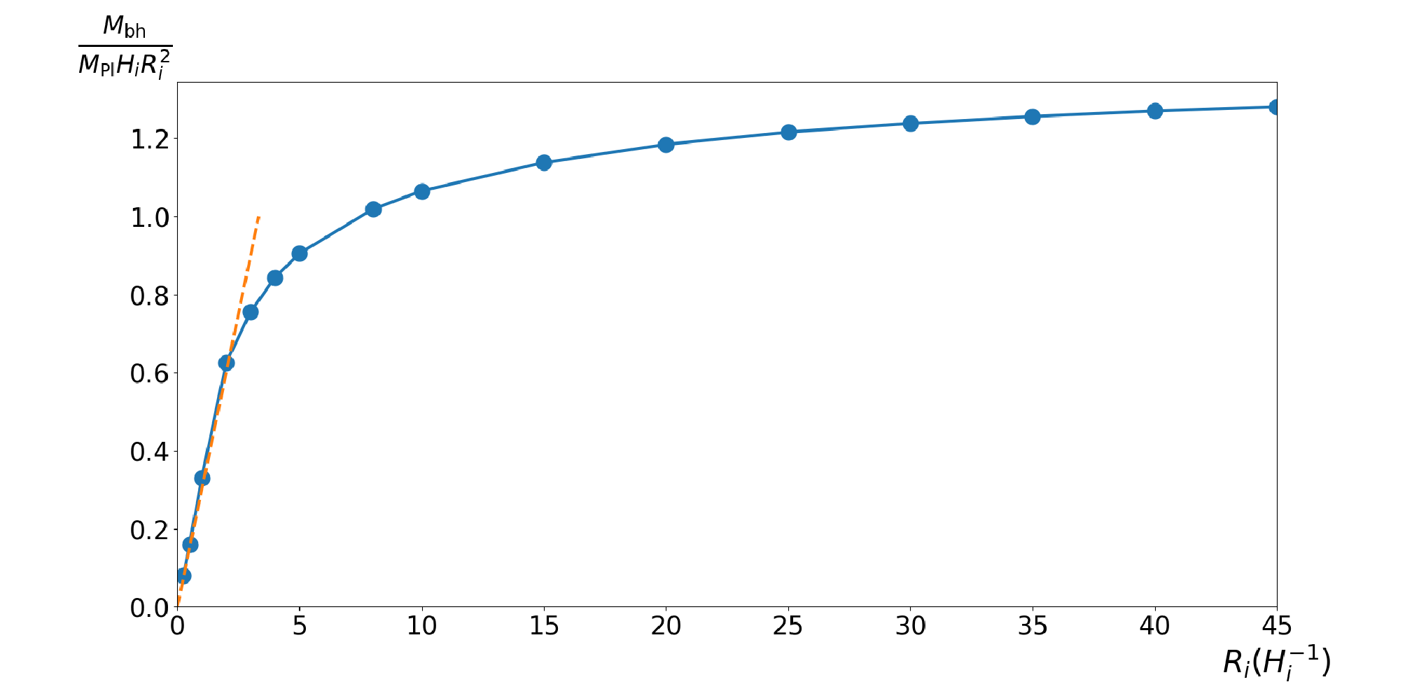
In Fig. 10 we plotted the ratio for a range of values of . We see that as increases, the ratio approaches a constant ,
| (32) |
Thus, for large values of the bound (6) is nearly saturated, as in the domain wall scenario.
The data points with correspond to subcritical regime, where we expect with defined from Eq.(4),
| (33) |
For the parameter values in Fig. 10, . This estimate is in agreement with the simulation results.
In conclusion, we can roughly approximate our results by setting
| (34) |
where the transition mass
| (35) |
corresponds to .
Parameters used in Fig. 10 give . In this case is not much different from but for other parameter values these two masses can be rather different. For example, if the first term in dominates, we have , which can be large for . Restricted by the capability of our simulation, we did not further explore the transition regime .

V Black hole mass spectrum
In earlier sections we have shown how a black hole could be formed by a vacuum bubble after inflation and how its mass is related to the initial bubble radius . During inflation the universe expands by a huge factor, so the bubble radii spread over a large range of scales. In this section we calculate the distribution of and find the resulting PBH mass spectrum. The calculation follows closely that in Ref. [16].
V.1 Size distribution of bubbles
To simplify the notation, in this subsection we use to denote the bubble radius during inflation.
The background spacetime during inflation can be described by a flat de Sitter metric,
| (36) |
with . Let be the bubble nucleation time. For simplicity, we assume that the bubble nucleates with a negligible radius compared to ; then the bubble worldsheet is well approximated by the future light cone of the nucleation point,
| (37) |
The number of bubbles that materialize in a coordinate interval and time interval is
| (38) |
where is the bubble nucleation rate per Hubble spacetime volume .
The number density of bubbles having radius in the interval at time is
| (39) |
where
| (40) |
is the physical volume element at .
The distribution (39) applies in the range , where is the number of inflationary e-folding. During inflation, the form of the distribution does not change with time, except the upper cutoff increases, reaching its maximum at the end of inflation.
V.2 Black hole mass distribution
To simplify the notation, in this and the next subsection we replace by .
By Eq. (39), the number density of bubbles within the radius range at the end of inflation is
| (41) |
After the bubble population is diluted by cosmic expansion, i.e.
| (42) |
where is the scale factor and we assume that the black holes are formed during the radiation era.
We use the standard definition of the mass function
| (43) |
where is the mass density of cold dark matter (CDM). Here can be interpreted as the mass density of black holes in the mass range . Since the black hole density and are diluted by the cosmic expansion in the same way, remains constant in time. The total fraction of CDM in PBHs can be expressed as
| (44) |
where is the PBH mass density.
During the radiation era , the dark matter density is of the order
| (45) |
where is a constant and is the dark matter mass within a Hubble radius at .
To find the mass function for our model, we use the simple ansatz (34) for . For bubbles with , we can neglect in Eq. (41). Then, for black holes with we have
| (46) |
and
| (47) |
For , we use , which gives and . Hence the resulting mass function has the form
| (48) |
The distribution (48) becomes inaccurate for black holes of mass
| (49) |
formed by bubbles with that nucleated during the last e-fold of inflation. For , Eq. (1) gives
| (50) |
If the first term dominates, ; if the second term dominates, then . In either case, the mass function decreases relatively fast at , and thus plays the role of a lower cutoff for the distribution (48).
Another cutoff mechanism is due to shape fluctuations of the bubbles.55 5 We are grateful to Jaume Garriga for emphasizing this to us. At the time of nucleation, bubbles are not perfectly spherical, because of quantum fluctuations. The amplitude of these fluctuations and their subsequent evolution have been discussed in Refs. [29, 30]. When a subcritical bubble collapses, the shape fluctuations grow and may become large before the bubble shrinks to its Schwarzschild radius. The bubble will then fragment into smaller pieces, which will in turn disintegrate into relativistic particles, so no black hole will be formed. We show in Appendix B that the corresponding lower bound on the black hole mass is
| (51) |
Some black holes with may still be formed from bubbles with atypically small shape fluctuations. We have not explored the mass distribution in this regime.
The shape fluctuations have no effect on the evolution of supercritical bubbles, thus the lower bound cannot be larger than . Therefore, the mass function (48) is effectively cut off at
| (52) |

Depending on the microphysical energy scales and , the mass parameters and can take a very wide range of values. For example, with and varying between the electroweak and grand unification scale, can be as small as a few grams and can be larger than the mass of the entire observable universe, while is restricted to . On the other hand, if the scale of is less than the electroweak scale, can be much larger. Here we shall treat and as free parameters. A general form of the mass function is illustrated in Fig, 11.
By Eq. (44), the total mass fraction of dark matter in PBH is given by
| (53) |
VI Observational properties and constraints
Apart from the distinctive mass spectrum, black holes produced by our mechanism have other interesting properties.
At the time of formation, these black holes are non-rotating. They may acquire some angular momentum by accretion of matter at later times, but much of the accretion occurs in the radiation era, within a few Hubble times after formation, and is likely to be nearly spherically symmetric. Hence we expect this population of black holes to be very slowly rotating. It is interesting to note that LIGO observations suggest low spins for the merging black holes [31] .
Scenarios of PBH formation from large primordial density fluctuations predict a background of stochastic gravitational waves, imposing significant constraints on this PBH formation mechanisms. Another stringent constraint comes from the observational bounds on the -distortion of the CMB spectrum. (For a discussion of these constraints, see, e.g. [32, 33] and references therein). Our model does not require large initial fluctuations and is not subject to these constraints.

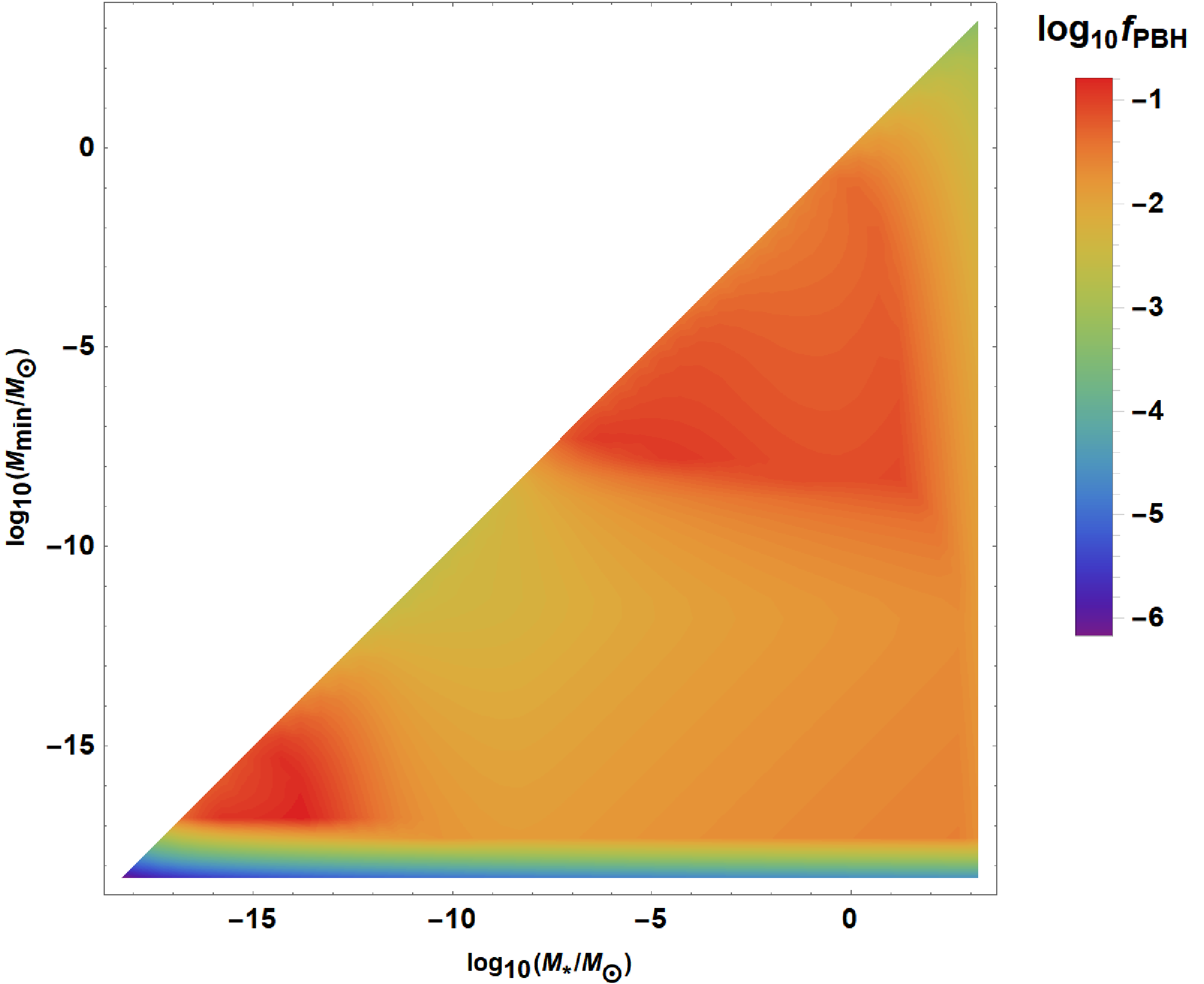
We now turn to observational constraints on our PBH formation model. Constraints on PBHs in different mass ranges have been extensively studied in the literature; see, e.g., [34] for an up to date review. We have indicated the current constraints in Fig. 12. A very stringent constraint on PBHs with comes from Hawking evaporation. For our mass function (48), a substantial mass fraction in PBHs can be obtained only if the cutoff mass is .
As discussed in Refs. [34, 35, 36], applying the constraints to models like ours, with a broad mass distribution of PBH, requires a special analysis. For example, observations like EROS, MACHO and HSC provide bounds over several orders of magnitude. For a "monochromatic" mass distribution, these bounds simply imply , but for an extended mass distribution they give a somewhat stronger constraint [36]
| (54) |
where is the range of masses covered by a particular observation. The resulting upper bound on the fraction of dark matter in PBHs () for different values of the model parameters and is shown in Fig. 13. It follows from the figure that PBHs in our model can at best constitute of order 10% of the dark matter.
Recent interest in PBHs is largely inspired by LIGO observations of gravitational waves emitted by inspiraling black holes with . It has been suggested in [37] that PBHs in this range of masses with could have a sufficient merger rate to account for LIGO results.66 6 Ref. [38] suggested that a significantly higher PBH density was required, . But recent detailed analysis in [39] supports the conclusions of [37]. This PBH density can in fact be achieved in our scenario. One example with and is shown in Fig. 12.
Another interesting possibility is that PBHs could serve as seeds for supermassive black holes (SMBH) observed at the galactic centers. The mass of such primordial seeds should be [41], and could be significantly higher. Their number density at present should be comparable to the density of large galaxies, . The relevant question for our scenario is then: What is the largest PBH we can expect to find in a galaxy?
The number density of PBHs of mass is approximately given by
| (55) |
For the mass function depends only on the nucleation rate , and requiring that we find . For (which is the upper bound of ), this is , which would certainly be sufficient to seed SMBH.
We thus see that for some values of the parameters black holes produced by high-energy bubbles can have interesting astrophysical implications. In particular, they could seed SMBH and could account for LIGO observations.
VII Conclusions and discussion
In this paper we used numerical simulations to study primordial black holes formed by vacuum bubbles created during inflation. At the end of inflation the bubbles have a scale-invariant size distribution, and we found in Eq. (34) how the black hole mass is related to the bubble radius. Bubbles smaller than certain critical size collapse to a Schwarzschild singularity; their mass has been estimated analytically in Ref. [16]. Supercritical bubbles, on the other hand, inflate in a baby universe, and [16] only found an upper bound on the black hole mass in this case. Here we confirmed the estimate of [16] for subcritical bubbles and showed that supercritical bubbles nearly saturate the upper bound on the black hole mass.
Black holes in this model have a very wide mass distribution, Eq.(48), stretching over many orders of magnitude. This distribution has a characteristic mass and has a distinctly different form at and . There is also a cutoff mass below which rapidly declines towards zero. Depending on the microphysics parameters, the characteristic mass can take a wide range of values, from less than a kilogram to much greater than .
The distribution at has the same form, , as that predicted in models where black holes are formed by scale-invariant density fluctuations in a radiation-dominated universe [28]. Black holes in this scenario are formed on the horizon scale, as in the supercritical regime of our model, so the coincidence of the mass functions is not surprising. We note, however, that the overdensity required for a horizon-size region of radiation to collapse is , and in order to form a substantial number of black holes the rms density fluctuations should be , much larger than that indicated by CMB and large-scale structure observations. For this reason, models predicting appreciable black hole formation from density fluctuations assume that the primordial fluctuation spectrum has an enhanced amplitude at relatively small scales (e.g., [32, 33]).
A mass distribution is also predicted in models closely related to ours, where PBH are formed by spherical domain walls [16, 17] or circular loops of cosmic string [14] formed during inflation. The domain wall model also has a characteristic mass above which black holes contain inflating baby universes. In the string model, the mass spectrum extends to very small masses and the black hole density is severely constrained by the Hawking radiation bound.
Considering the constraints from different observations, we found an upper bound on the fraction of dark matter in PBHs in our model, shown in Fig. 13. PBHs here can constitute no more than about 10% of the dark matter. Furthermore, we found that the fraction of dark matter in PBHs with mass is which implies that the black holes detected in LIGO events could be the PBHs of our model. With a large number of future merger detections, we should be able to infer the black hole mass spectrum (e.g., [40]) and to confirm or rule out our PBH formation mechanism.
We also determined an upper bound on the mass of the largest PBH that one can expect to find in a large galaxy, . This shows that PBHs of our model can serve as seeds of supermassive black holes (SMBH) observed at the galactic centers. There is in fact a range of parameters for which the model can account for both SMBH and LIGO observations.
Black holes formed by vacuum bubbles can have significant observational effects only if the bubble nucleation rate is relatively high, . This corresponds to the tunneling action , while the typical value is . We note, however, that in the string landscape scenario the false vacuum has a large number of decay channels, and it seems likely that some of them may have small barriers with a relatively high tunneling probability.
Our analysis in this paper is based on several simplifying assumptions. To begin with, we assumed that the vacuum energy is instantaneously thermalized at the end of inflation. In a more realistic model, thermalization may extend over several Hubble times and may be preceded by a period of the inflaton field oscillations characterized by the dust equation of state. We also assumed that the bubble radius at nucleation is much smaller than the Hubble horizon.
These assumptions, however, affect only the low-mass end of the black hole distribution, . Perhaps more consequential is the assumption that thermalized matter particles cannot penetrate the bubble and are reflected from the bubble wall. This is likely to be true for particles with energies lower than the symmetry breaking scale of the bubble, , but at higher energies the wall may be transparent to the particles [42].
We also assumed that the bubble wall tension and the bubble nucleation rate are constant parameters. However, this is not generally the case. When the bubble is formed, the wall tension is determined by the shape of the barrier between the inflating false vacuum of energy density and the vacuum in the bubble interior of energy density . On the other hand, at the end of inflation the barrier is between our vacuum of very low energy density and the bubble interior. This means that the shape of the barrier and the wall tension can change significantly in the course of inflation.
The bubble nucleation rate may also change during inflation. As the inflaton field rolls downhill, it moves relative to the minimum at , so the tunneling path (and therefore the tunneling action) are also changing. As a result the mass distribution of black holes could be significantly modified and could develop a peak at the value of that corresponds to the smallest tunneling action. We leave the analysis of these possibilities for future research.
Acknowledgements.
This work was supported by the National Science Foundation under grant 1518742. H.D. was also supported by Burlingame Fellowship at Tufts University. We are grateful to Jaume Garriga and Andrei Gruzinov for very useful discussions and to Vladyslav Syrotenko for his participation at the early stages of this project. We would also like to thank Bernard Carr for useful comments on the manuscript, and Xiaozhe Hu for helpful advice on some simulation issues.Appendix A
In this appendix we use Israel’s junction conditions to find the conditions needed for simulations. We closely follow the method and notation in [43].
The interior of the vacuum bubble can be described by de Sitter spacetime with metric
| (56) |
where with the Hubble constant. We assume that outside the bubble
| (57) |
where , and are functions of and .
Let the trajectory of the wall be or , where is the wall proper time. If the wall is comoving for an exterior observer, , where . The tangent vector to the wall hypersurface is , and . Assuming to be positive, gives Let be a unit vector normal to the wall hypersurface; then and , which give and .
We define the brackets , and . Here "in" and "out" respectively denote the value of right inside and outside the wall. Then Israel’s first junction condition is , where is the induced metric at the wall. The second junction condition is , where is the extrinsic curvature at the wall, is the energy-momentum tensor of the wall, with the surface energy density (or tension).
The equation of motion for the wall is given by
| (58) |
where is the 4-velocity of the fluid. Inside the bubble .
We shall now use the junction conditions and Eq.(A3) to derive some relations that will be useful for setting up the boundary condition for our simulations.
By the first junction condition, at the wall. Taking the derivative of with respect to gives
| (59) |
Let Then at the wall can be written as
| (60) |
The component of the second junction condition gives
| (61) |
Right outside the wall, we have
| (62) |
while
| (63) |
Then by Eq. (61), at the wall can be written as
| (64) |
The component of the second junction condition gives
| (65) |
where with the Chistoffel symbols for the 4-spacetime. Right outside the wall,
| (69) |
This is used as the boundary condition in the simulations.
We can also obtain an explicit form of the equation of motion for the wall. It can be shown that
| (71) |
Appendix B
Vacuum bubbles can deviate from spherical shape due to quantum fluctuations. The unperturbed worldsheet of the bubble wall is a -dimensional de Sitter space with a Hubble parameter
| (72) |
where is the difference of vacuum energy densities outside and inside the bubble, and is the tension of the bubble wall. The magnitude of fluctuations of the bubble radius was estimated in Ref. [30]:
| (73) |
As the bubble expands, remains constant, so the ratio decreases and the bubble becomes more and more spherical. Here is the bubble radius.
This analysis, however, did not account for gravitational effects. When the bubble radius gets larger than the de Sitter horizon of the exterior inflating universe, , we expect that the shape of the bubble "freezes" and it is conformally stretched afterwards.77 7 More exactly, we expect fluctuations of wavelength to freeze when gets larger than . But here we are interested in the lowest multipoles, so is comparable to the bubble radius. The shape fluctuations are then given by
| (74) |
Assuming that , this is of the order
| (75) |
Widrow [44] studied perturbations on collapsing domain walls and found that the fluctuation remains approximately constant in the course of collapse. We will show that this also holds for collapsing bubbles later in this Appendix.
A black hole is formed if . Let us first assume that the bubble energy at the moment of maximal expansion is dominated by the interior vacuum energy,
| (76) |
Requiring that , we have
| (77) |
and
| (78) |
Substituting this into (76) we obtain
| (79) |
If , and are characterized by the same energy scale , this gives
| (80) |
This is a rather weak constraint. For example, if is the electroweak scale, it gives kg. On the other hand, the cutoff mass can be relatively large when .
Bubble collapse
Let us now show that the evolution of perturbations on a collapsing bubble is similar to that on a collapsing domain wall.
Let us first consider collapse of a spherical bubble. We start with the conserved mass,
| (81) |
where the overdot stands for a derivative with respect to proper time . Suppose the bubble is initially at rest, , at the maximal expansion radius, . We will be interested in the asymptotic behavior, when .
In this regime, the terms proportional to on the right hand side of (81) become negligible and , so Eq. (81) reduces to
| (82) |
where the "-" sign is chosen because we are considering the collapse.
The solution of Eq. (82) is
| (83) |
Here, we choose the origin of so that at the moment of collapse; then prior to the collapse. It follows from (83) that the total proper time it takes for the bubble to collapse is
| (84) |
Fluctuations on the collapsing bubble are described by a scalar field living at the bubble wall and satisfying the equation
| (85) |
The field has a tachyonic mass, , and a non-minimal coupling to the 3-curvature on the wall worldsheet,
| (86) |
The worldsheet metric can be written as
| (87) |
Then, with the solution (83) the 3-curvature becomes
| (88) |
where the last approximation applies for .
The tachyonic mass could in principle lead to an instability. But the timescale for such an instability to develop is , and we see from (84) that there is not enough time. In fact, the mass term in Eq. (85) is negligible to compared to the curvature term for . Neglecting this term and using the approximation (88), we rewrite Eq. (85) as
| (89) |
This has solutions with . The dominant solution is
| (90) |
It was shown in [29] that the rms fluctuation of the bubble wall is related to as , where is the Lorentz factor of the wall. (The factor of accounts for the effect of Lorentz contraction of bubble fluctuations.) Then Eq. (90) tells us that the fluctuation amplitude does not change in the course of collapse:
| (91) |
This agrees with the result obtained by Widrow [44] for collapsing domain walls. The agreement between the two cases is not surprising, since the vacuum energy density becomes dynamically unimportant at .
References
- [1] Ya. B. Zeldovich and I.D. Novikov, Sov. Phys. Astron. J. 10, 602 (1967).
- [2] S. Hawking, “Gravitationally collapsed objects of very low mass,” Mon. Not. Roy. Astron. Soc. 152, 75 (1971).
- [3] B. J. Carr and S. W. Hawking, “Black holes in the early Universe,” Mon. Not. Roy. Astron. Soc. 168, 399 (1974).
- [4] B. J. Carr and J. E. Lidsey, “Primordial black holes and generalized constraints on chaotic inflation,” Phys. Rev. D 48, 543 (1993).
- [5] J. García-Bellido, A. D. Linde and D. Wands, “Density perturbations and black hole formation in hybrid inflation,” Phys. Rev. D 54, 6040 (1996) [astro-ph/9605094].
- [6] J. Yokoyama, “Formation of MACHO primordial black holes in inflationary cosmology,” Astron. Astrophys. 318, 673 (1997) [astro-ph/9509027].
- [7] P. H. Frampton, M. Kawasaki, F. Takahashi and T. T. Yanagida, “Primordial Black Holes as All Dark Matter,” JCAP 1004, 023 (2010) [arXiv:1001.2308 [hep-ph]].
- [8] S. Clesse and J. García-Bellido, “Massive Primordial Black Holes from Hybrid Inflation as Dark Matter and the seeds of Galaxies,” Phys. Rev. D 92, no. 2, 023524 (2015) [arXiv:1501.07565 [astro-ph.CO]].
- [9] H. Kodama, M. Sasaki and K. Sato, “Abundance of Primordial Holes Produced by Cosmological First Order Phase Transition,” Prog. Theor. Phys. 68, 1979 (1982).
- [10] K. Jedamzik and J. C. Niemeyer, “Primordial black hole formation during first order phase transitions,” Phys. Rev. D 59, 124014 (1999) [astro-ph/9901293].
- [11] M. Y. Khlopov, R. V. Konoplich, S. G. Rubin and A. S. Sakharov, “First order phase transitions as a source of black holes in the early universe,” Grav. Cosmol. 2, S1 (1999) [hep-ph/9912422].
- [12] S. W. Hawking, “Black Holes From Cosmic Strings,” Phys. Lett. B 231, 237 (1989).
- [13] A. Polnarev and R. Zembowicz, “Formation of Primordial Black Holes by Cosmic Strings,” Phys. Rev. D 43, 1106 (1991).
- [14] J. Garriga and A. Vilenkin, “Black holes from nucleating strings,” Phys. Rev. D 47, 3265 (1993) [hep-ph/9208212].
- [15] M. Y. Khlopov, S. G. Rubin and A. S. Sakharov, “Primordial structure of massive black hole clusters,” Astropart. Phys. 23, 265 (2005) [astro-ph/0401532].
- [16] J. Garriga, A. Vilenkin and J. Zhang, “Black holes and the multiverse,” JCAP 1602, no. 02, 064 (2016) [arXiv:1512.01819 [hep-th]].
- [17] H. Deng, J. Garriga and A. Vilenkin, “Primordial black hole and wormhole formation by domain walls,” JCAP 1704, no. 04, 050 (2017) [arXiv:1612.03753 [gr-qc]].
- [18] S. R. Coleman and F. De Luccia, “Gravitational Effects on and of Vacuum Decay,” Phys. Rev. D 21, 3305 (1980).
- [19] V. A. Berezin, V. A. Kuzmin and I. I. Tkachev, “Thin Wall Vacuum Domains Evolution,” Phys. Lett. B 120, 91 (1983).
- [20] S. K. Blau, E. I. Guendelman and A. H. Guth, “The Dynamics of False Vacuum Bubbles,” Phys. Rev. D 35, 1747 (1987).
- [21] J. Bloomfield, D. Bulhosa and S. Face, “Formalism for Primordial Black Hole Formation in Spherical Symmetry,” arXiv:1504.02071 [gr-qc].
- [22] C. W. Misner and D. H. Sharp, “Relativistic equations for adiabatic, spherically symmetric gravitational collapse,” Phys. Rev. 136, B571 (1964).
- [23] S. A. Hayward, “Gravitational energy in spherical symmetry,” Phys. Rev. D 53, 1938 (1996) [gr-qc/9408002].
- [24] V. Faraoni, “Cosmological and black hole apparent horizons,” Vol. 907. Springer (2015).
- [25] T. W. Baumgarte and S. L. Shapiro, “Numerical relativity: solving Einstein’s equations on the computer,” Cambridge University Press (2010).
- [26] M. Liebendoerfer, S. Rosswog and F. K. Thielemann, “An Adaptive grid, implicit code for spherically symmetric, general relativistic hydrodynamics in comoving coordinates,” Astrophys. J. Suppl. 141, 229 (2002) [astro-ph/0106539].
- [27] J. Von Neumann and R. Richtmyer, “A method for the numerical calculation of hydrodynamic shocks,” J. Appl. Phys. 21, no. 3 (1950).
- [28] B. J. Carr, “The Primordial black hole mass spectrum,” Astrophys. J. 201, 1 (1975).
- [29] J. Garriga and A. Vilenkin, “Perturbations on domain walls and strings: A Covariant theory,” Phys. Rev. D 44, 1007 (1991).
- [30] J. Garriga and A. Vilenkin, “Quantum fluctuations on domain walls, strings and vacuum bubbles,” Phys. Rev. D 45, 3469 (1992).
- [31] K. Hotokezaka and T. Piran, “Are the observed black hole mergers spins consistent with field binary progenitors?,” arXiv:1707.08978 [astro-ph.HE].
- [32] K. Inomata, M. Kawasaki, K. Mukaida, Y. Tada and T. T. Yanagida, “Inflationary primordial black holes for the LIGO gravitational wave events and pulsar timing array experiments,” Phys. Rev. D 95, no. 12, 123510 (2017) [arXiv:1611.06130 [astro-ph.CO]].
- [33] J. García-Bellido, M. Peloso and C. Unal, “Gravitational Wave signatures of inflationary models from Primordial Black Hole Dark Matter,” arXiv:1707.02441 [astro-ph.CO].
- [34] B. Carr, F. Kuhnel and M. Sandstad, “Primordial Black Holes as Dark Matter,” Phys. Rev. D 94, no. 8, 083504 (2016) [arXiv:1607.06077 [astro-ph.CO]].
- [35] F. Kühnel and K. Freese, “Constraints on Primordial Black Holes with Extended Mass Functions,” Phys. Rev. D 95, no. 8, 083508 (2017) [arXiv:1701.07223 [astro-ph.CO]].
- [36] B. Carr, M. Raidal, T. Tenkanen, V. Vaskonen and H. Veermäe, “Primordial black hole constraints for extended mass functions,” Phys. Rev. D 96, no. 2, 023514 (2017) [arXiv:1705.05567 [astro-ph.CO]].
- [37] M. Sasaki, T. Suyama, T. Tanaka and S. Yokoyama, “Primordial Black Hole Scenario for the Gravitational-Wave Event GW150914,” Phys. Rev. Lett. 117, no. 6, 061101 (2016) [arXiv:1603.08338 [astro-ph.CO]].
- [38] S. Bird, I. Cholis, J. B. Muñoz, Y. Ali-Haïmoud, M. Kamionkowski, E. D. Kovetz, A. Raccanelli and A. G. Riess, “Did LIGO detect dark matter?,” Phys. Rev. Lett. 116, no. 20, 201301 (2016) [arXiv:1603.00464 [astro-ph.CO]].
- [39] Y. Ali-Haïmoud, E. D. Kovetz and M. Kamionkowski, “The merger rate of primordial-black-hole binaries,” arXiv:1709.06576 [astro-ph.CO].
- [40] M. Zevin, C. Pankow, C. L. Rodriguez, L. Sampson, E. Chase, V. Kalogera and F. A. Rasio, “Constraining Formation Models of Binary Black Holes with Gravitational-Wave Observations,” Astrophys. J. 846, no. 1, 82 (2017) [arXiv:1704.07379 [astro-ph.HE]].
- [41] N. Duechting, “Supermassive black holes from primordial black hole seeds,” Phys. Rev. D 70, 064015 (2004) [astro-ph/0406260].
- [42] A. E. Everett, “Observational consequences of a ’domain’ structure of the universe,” Phys. Rev. D 10, 3161 (1974).
- [43] N. Tanahashi and C. M. Yoo, “Spherical Domain Wall Collapse in a Dust Universe,” Class. Quant. Grav. 32, no. 15, 155003 (2015) [arXiv:1411.7479 [gr-qc]].
- [44] L. M. Widrow, “The Collapse of Nearly Spherical Domain Walls,” Phys. Rev. D 39, 3576 (1989).