The Impact of baryonic physics on the kinetic Sunyaev-Zel’dovich Effect

The relative change in the CMB temperature induced by the kSZ effect in the direction of the line-of-sight unit vector $\hat{\gamma}$ is

where $\mathbf{v}_{e}$ is the peculiar velocity field of the electrons, $\tau$ is the (inhomogeneous) Thompson optical depth between $z=0$ and the scatterer, where $d\tau=c~n_{e}\sigma_{T}dt$. In the post-reionization universe, the IGM is nearly fully ionized and $n_{e}$ closely follows the underlying gas density field. We define the free electron number density contrast by

in terms of the global average of the electron density $\bar{n}_{e}$. Defining the specific momentum (henceforth referred to as “momentum”) $\mathbf{q}\equiv\mathbf{v}_{e}[1+\delta_{e}]$ allows us to rewrite Equation (1) as

where $s(z)$ is the comoving distance to the scatterer and $\bar{n}_{e,a0}\equiv\bar{n}_{e,a}(z=0)$ is the current redshift 0 value of the mean number density of free plus bound electrons, $\bar{n}_{e,a}(z)\equiv(1-Y_{P}/2)\bar{\rho}_{b}(z)/m_{p}$. The mean baryon number density is $\rho_{b}(z)/m_{p}$, where $\bar{\rho}_{b}(z)=[3H_{0}^{2}\Omega_{b}(1+z)^{3}]/[8\pi G]$ is the global baryonic mass-density of the universe and $m_{p}$ is the proton mass. We set the primordial helium abundance to $Y_{P}=0.24$; the small metal contamination for these average numbers is ignored. We define the fraction of free electrons to be $f_{e}(z)\equiv\bar{n}_{e}/\bar{n}_{e,a}$. Thus if Helium is fully ionizes as well as hydrogen $f_{e}$ would be unity.

As mentioned in the introduction, the Fourier transform of the momentum, $\tilde{\mathbf{q}}\equiv\int d^{3}\mathbf{x}~e^{i\mathbf{k}\cdot\mathbf{x}}\mathbf{q}(\mathbf{x})$, can be separated into the transverse component, $\tilde{\mathbf{q}}_{\perp}\equiv\tilde{\mathbf{q}}-\mathbf{k}[\tilde{\mathbf{q}}\cdot\mathbf{k}]$, which is perpendicular to the wavevector, and the longitudinal component, $\tilde{\mathbf{q}}_{\parallel}\equiv\mathbf{k}[\tilde{\mathbf{q}}\cdot\mathbf{k}]$, which is parallel to the wavevector. In the kSZ angular power spectrum of $\Delta T/T$, $\tilde{\mathbf{q}}_{\parallel}$ gives a negligibly small contribution compared to that from $\tilde{\mathbf{q}}_{\perp}$ [33, 41, 40], though it dominates the $\Delta T/T$ primary anisotropies during recombination and at low multipoles $\ell<10$ through reionization. Thus we can write the CMB angular power spectrum in terms of the transverse component only:

[33]. Thus $f_{e}(z)$ and $P_{q_{\perp}}(k,z)$ are the key quantities that determine the shape and amplitude of the kSZ power spectrum for a fixed background cosmology.

Here, we shall summarize the derivation of $P_{q_{\perp}}$ in terms of the density and velocity power spectra. In Fourier space

where $\tilde{\mathbf{q}}=\int d^{3}\mathbf{x}~e^{i\mathbf{k}\cdot\mathbf{x}}\mathbf{q}(\mathbf{x})$ .

The first term can have non-zero curl only in the nonlinear regime, but its contribution is below a percent level [37, P16]. The transverse power spectrum from the second order term, $\int\delta v$, gives

where $P_{\delta\delta vv}$ is given by

In the linear regime, all of the four fields in the bracket, $\left<\delta\delta vv\right>$, are Gaussian if the initial conditions are. This allows us to expand the whole bracket into brackets with two fields using Wick’s theorem: $\left<ABCD\right>_{uc}=\left<AB\right>\left<CD\right>+\left<AC\right>\left<BD\right>+\left<AD\right>\left<BC\right>$. In the post-reionization regime, however, nonlinearity creates non-Gaussianity in the density and velocity fields, which gives a rise to the connected term, $\left<ABCD\right>_{c}$.

The unconnected part is given by

where $\mu^{\prime}\equiv\hat{\mathbf{k}}\cdot\hat{\mathbf{k}^{\prime}}$. Instead of the above expression, the following approximate expression is often used since it is highly accurate and convenient to evaluate [36, P16].

For higher wavenumbers $k\gtrsim 0.1~h~\rm{Mpc}^{-1}$ the kSZ signal is still quite relevant, and most of the contribution in the above integral comes from the coupling of $P_{vv}(k^{\prime})$ at $k^{\prime}\lesssim 0.1~h~\rm{Mpc}^{-1}$ with $P_{\delta\delta}(|\mathbf{k}-\mathbf{k^{\prime}}|)\approx P_{\delta\delta}(k)$. While linear calculations are accurate enough for $P_{vv}$, we need a more accurate $P_{\delta\delta}$ to account for nonlinear effects at high $k$’s.

At $z\lesssim 3$ and $k>1~h~\rm{Mpc}^{-1}$, $P_{\delta\delta}$ is strongly affected by both the growth of nonlinear structure, which can differ for gas cf. dark matter, and the baryonic physics operating. We characterize how the electron density power $P^{e}_{\delta\delta}$ differs from the dark matter power $P^{d}_{\delta\delta}$ by a scale and redshift dependent bias, defined here by

To see the combined effects in both $f_{e}$ and $P_{q_{\perp}}$, Shaw et al. [39] (hereafter SRN12) introduced a window function,

which we adopt in this work to describe the baryonic effects.

We note that $P_{q_{\perp},uc}$ does not fully account for $P_{q_{\perp}}$ in the nonlinear regime due to the rise of the connected term, $P_{q_{\perp},c}$. P16 confirmed that it is present and important to include for the pure dark matter momentum field. We find the connected term is still important for the electrons, but differs in detail because of the relative bias.

We show the power spectra of dark matter ($P^{d}_{\delta\delta}$) and free electron ($P^{e}_{\delta\delta}$) density fields in the right panels of Figure 1 for $z=0,~1,~3,$ and 5. Nonlinearity results in the familiar result of $P^{d}_{\delta\delta}$ growing faster than the linear theory prediction. At $k>1~h~\rm{Mpc}^{-1}$, $P^{d}_{\delta\delta}$ is about an order of magnitude larger than the linear prediction at $z=0$. As is well known from previous works, the HALOFIT model of Smith et al. [47] does a good job in modeling this enhancement. The evolution of $P^{e}_{\delta\delta}$, however, is more complicated, showing the effects of dynamical nonlinear growth at $z\geq 3$, but complicated by separation of gas from baryons by shocking and feedback, combining to give a growth slower than linear after $z=3$. How this difference between $P^{d}_{\delta\delta}$ and $P^{e}_{\delta\delta}$ arises due to the effects of baryonic physics of plasma is what we aim to probe.

A list of relevant baryonic physics that will impact the free electrons relative to the dark matter are:

• 1)

  Collapse of cooled gas

• 2)

  Star-formation converting gas into stars and blackholes

• 3)

  AGN feedback blowing gas out of potential wells

• 4)

  Self-shielding of cold neutral gas in galaxies against ionizing radiation

• 5)

  He II reionization at $z\sim 3$

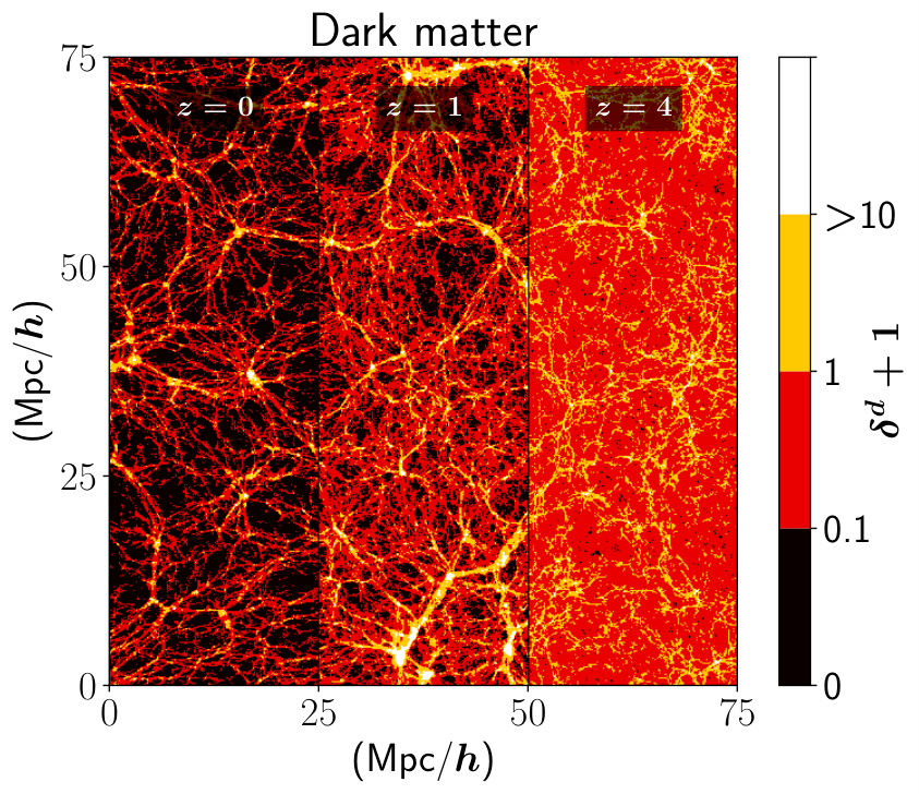
For example, the density map of free electron in comparison to that of dark matter (See the left panels of Figure 1) shows the smoothing of the electron density field at $\bm{z\leq 1}$ at certain scales that we can attribute to the effect of AGN feedback. The spread extends over larger scales than in some other gasdynamical calculations, a consequence of the strong feedback in Illustris. This explains the deficit in $P^{e}_{\delta\delta}$ compared to $P^{d}_{\delta\delta}$ at high $k$ and low redshift. To further analyze the differences, we now explore the window function $W_{e}$ (Eq. 11).

The window function for the free electrons relative to dark matter $W_{e}$ encodes the effect of all of the baryonic physics relevant to the intergalactic plasma. To help deconstruct its shape we explore equivalent window functions for baryons ($W_{b}$) and gas ($W_{g}$) as well, defined similarly to $W_{e}$, except that we use baryon and gas densities are used instead of electron number density in Equation (2). The baryon density field includes all the mass in stars, AGNs and neutral gas as well as gas and we can thus use it to exclude the effect of converting gas into those elements that do not give rise to the kSZ effect. The gas density field does include neutral gas in galaxies, but not stars or AGNs, which allows us to decompose the effect of having multiphase gas. We show $W_{b},~W_{g},$ and $W_{e}$ in Figure 3 for $z=0,~0.5,~1,~2,$ and 4.

In $W_{b}$ an up-turn appears at $k\sim 5~h~\rm{Mpc}^{-1}$ at all redshifts shown, a trend easily understood by the collapse of gas on small scales following gas cooling in over-dense regions. At $z\leq 2$, the feedback of star-formation and AGNs heats the gas and makes it expand over time, damping $W_{b}$ at $k\gtrsim 0.3~h~\rm{Mpc}^{-1}$. The combination of these two effects creates a dipper-like shape in $W_{b}^{2}$ at $z\leq 1$.

The comparison of $W_{g}$ to $W_{b}$ demonstrates the effect of star-formation. As gas is converted into stars in density peaks, gas density power is strongly suppressed at $k\gtrsim 1~h~\rm{Mpc}^{-1}$. As a result, the up-turn at high-$k$ is much weaker in $W_{g}$. Additionally, star-formation suppresses $W_{g}$ at all wavenumbers as can be seen from the low-$k$ limit of $W^{2}_{g}$ being less than one. For the case in which a fraction $(1-f_{g})$ of gas was of converted into stars homogeneously, $W_{g}^{2}$ would be suppressed by a factor of $f_{g}^{2}$. In Illustris we find $W^{2}_{g}$ drops below $f_{g}^{2}$ at low $k$ because star-formation drains gas preferentially in over-densities and create an anti-bias in the gas density field. The bias of the gas density $b_{g}$ shown in the middle right panel of Figure 3 clearly shows this anti-biasing effect in its low-$k$ limit. To extract the anti-bias, we define $b_{g0}$ as $W_{g}(k\rightarrow 0)$. In Figure 4 we plot $b^{2}_{g0}$, $f^{2}_{g}$, $f^{2}_{g}b^{2}_{g0}$ and their counterparts for electron density. Due to ongoing star-formation, $f^{2}_{g}$ monotonically decreases from 0.92 to 0.8 between $z=5$ and $0$. $b_{g}^{2}$ starts from 0.96 at $z=0$ and decreases until $z=1$ down to 0.92 and stays without much change until $z=0$. The combination of these two term, $f^{2}_{g}b^{2}_{g0}$, gives a large-scale suppression effect that grows from $5\%$ to $20\%$ between $z=5$ and $0$.

$W_{e}$ has additional suppression effects on top of what it inherits from $W_{g}$ because not all electrons that survived star-formation contribute to the mean ionized plasma: a significant fraction of them are trapped in the cold neutral gas in galaxies that remains self-shielded from extragalactic ionizing radiation or are locked in helium atoms at $z\gtrsim 3$ where most heliums are only singly ionized even when hydrogen is ionized. Similarly to the comparison of $W_{g}$ to $W_{b}$, $W_{e}$ gets an all-wavenumber suppression plus more high-$k$ suppression compared to $W_{g}$, which makes $W_{e}<W_{g}$ at all scales. The filled circles on the curves for $W_{e}$ denote the wavenumber that contributes mostly to the $\ell=3000$ signal at give $z$, $\ell/s(z)$. Those circles show that the signal down to $z=2$ is mostly affected by the large-scale term $f^{2}_{g}b^{2}_{g0}$ and the $z<2$ signal is further suppressed by the AGN feedback.

We have paid considerable attention to the deconstruction of the total kSZ power into some of its two point subcomponents, in particular targeting how the $\langle\delta\delta\rangle$ terms vary relative to each other for the electron density, gas density and dark matter through the power ratios $b^{2}_{e}=P^{e}_{\delta\delta}/P^{d}_{\delta\delta}$ and $b^{2}_{g}=P^{g}_{\delta\delta}/P^{d}_{\delta\delta}$, Fourier transforms of the position-position correlations $[\langle\delta_{e}\delta_{e}\rangle\langle\delta_{d}\delta_{d}\rangle^{-1}](\mathbf{x}-\mathbf{x}^{\prime})$ and $[\langle\delta_{g}\delta_{g}\rangle\langle\delta_{d}\delta_{d}\rangle^{-1}](\mathbf{x}-\mathbf{x}^{\prime})$. Of interest as well are statistically averaged values of $n_{e}$ and $\rho_{g}$ subject to the constraint of $\rho_{d}$. This is a nonlinear relationship which involves averaging over constrained probability functionals to yield $\langle\delta_{e}(\mathbf{x})|\delta_{d}\rangle$ and $\langle\delta_{g}(\mathbf{x})|\delta_{d}\rangle$. However there is a “linear response” limit in which, e.g.,

The (suitably normalized) susceptibility of $n_{e}$ to $\rho_{d}$ is $\chi_{ed}$, with units of inverse volume; the name is chosen because there is a clear relation to the familiar susceptibilities that relate electric and magnetic polarizabilities to applied electromagnetic fields, ultimately leading to dielectric tensors. Another terminology for $\chi_{ed}$ is response function, for obvious reasons.

In the halo model expansion for the dark matter density, there are susceptibilities for each class of halo, giving the response of $\delta_{d}$ to $M_{h}n_{h}$, where $M_{h}$ is the halo mass and $n_{h}$ the halo number density for that class. In that case, the susceptibilities give the (suitably normalized) mean dark matter profile of the halo class. Usually scalings are done to take out the dominant dependences on the overall size of the halo (or equivalently the overall mass). Thus these ideas are familiar. The Fourier transform $\tilde{\chi}_{eh}(k)$ is the electron density form factor of the halo.

We can relate these ideas to what is done in practice to make mock maps of the kSZ effect, e.g., in the peak patch approach for creating deep all-sky halo catalogs [48], [49], and [50], with analytic or measured susceptibilities used to ”paint on” the electron density profiles around halos. The velocities for the halos are automatic outputs in the peak patch catalog, suitably smoothed over the cluster scale, which changes from cluster to cluster. In [50] the susceptibilities are determined by measurement in the BBPS cosmic hydro simulations of [51], constructing stacked profiles for halos with specified mass and redshift bins, each bin defining a halo-class. The product of the electron density profile and the velocity allows for all-sky mocks of the kSZ effect. The accuracy of the mock then depends upon the magnitude of the residual fluctuations about the mean-field linear-response expansion inherent in this “halo model” for $n_{e}$.

The Illustris simulations could also be used to calculate the electron density response for each of the halo bins, and be incorporated into the peak-patch simulator in the same way as the BBPS calculations have been. The resolution of Illustris was much superior to BBPS, which has allowed us to study here the influence of galactic-scale baryonic physics that are not resolved in the BBPS simulations, although star and AGN feedback were incorporated. On the other hand, the Illustris box was smaller, and only one box was run, limiting statistical inferences. Thus in Illustris the rare-mass clusters are fewer, exacerbated because there was only one realization. (BBPS ran a (small) ensemble of simulations.) While we await more and larger Illustris and other high resolution simulations for susceptibility measurements, we shall content ourselves here with $\chi_{ed}$ measurements, estimated by cross-correlations weighted by the inverse of the self-clustering correlation matrix for dark matter $<\delta_{e}\delta_{d}><\delta_{d}\delta_{d}>^{-1}$:

For halos $\tilde{\chi}_{dh}(k)$ approaches a mass-weighted anti-bias $b_{dh0}$ for the halo-class in question at low $k$, $\delta_{d}\sim\delta_{h}/b_{hd0}$, with $b_{hd0}=\tilde{\chi}_{hd}(k\rightarrow 0)$ the usual mass-halo dependent bias of halos relative to dark matter density, with $b_{hd0}>1$. By analogy, we can think of the dimensionless $\tilde{\chi}_{ed}(k)$ as the scale-dependent bias of electron density relative to dark matter density.

In the susceptibility language, $b^{2}_{e}=P^{e}_{\delta\delta}/P^{d}_{\delta\delta}=\tilde{\chi}_{ed}(k)/\tilde{\chi}_{de}(k)$, hence asymptotically approaches $b_{ed0}/b_{de0}$. Although naive biasing prescriptions would suggest this approaches $b_{ed0}^{2}$, in practice it is not quite true: we do not have $\tilde{\chi}_{de}(k)=1/\tilde{\chi}_{ed}(k)$, so $b_{e}$ also does not reduce to the biasing factor of $e$ relative to $d$. However as we show in Fig. 5 the basic features of $b_{e}$ look rather similar to those of $\tilde{\chi}_{ed}$, though with different high $k$ suppression behavior.

$P_{q_{\perp},uc}$ (Eq. 9) was often assumed to represent the complete $P_{q_{\perp}}$ in previous literature. SRN12 and Zhang et al. [38] showed that evaluating Equation (9) using density power spectrum from simulations and directly computing $P_{q_{\perp}}$ gave nearly similar results. P16 recently revisited that comparison with a pure dark matter simulation and found that $P_{q_{\perp}}$ can be larger than $P_{q_{\perp},uc}$ up to $\sim 30\%$ at $k\gtrsim 1~h~\rm{Mpc}^{-1}$ due to the connected term in $P_{q_{\perp}}$ arising in the nonlinear regime. We shall check on this issue for the free electron momentum field here.

To measure $P_{q_{\perp}}$ directly from Illustris, we first assign the velocity-weighted electron number of each particle to a nearest grid in a $512^{3}$ mesh. Taking the power spectrum of this mesh would however underestimate $P_{q_{\perp}}$ because it misses velocity modes larger than the size of the simulation box ($75~h^{-1}~\rm{Mpc}$) and we thus need to correct for the missing velocity modes not included in the box. We describe how we estimate the correction for those missing modes in the Appendix and show the expression in Equation (A1). In the rest of the paper, we shall use the missing-power-correction-added power spectrum in the analysis and denote it as $P_{q_{\perp},tot}$.

In Figure 6, we plot the ratio of $P_{q_{\perp},tot}$, and the unconnected part of the spectrum, $P_{q_{\perp},uc}$, to see if $P_{q_{\perp},uc}$ can fully explains the spectrum. $P_{q_{\perp},uc}$ is calculated by evaluating Equation (9) with the density and velocity power spectra of Illustris. We focus on the higher $k>0.5~h~\rm{Mpc}^{-1}$ wavenumbers where the kSZ signal is quite relevant and the number of plane-waves in the simulation box are sufficient for good statistically sampling.

At $z=47$ where the dark matter density and velocity fluctuations are in the linear regime, $P_{q_{\perp},tot}$ agrees with $P_{q_{\perp},uc}$ within a percent. At $z\leq 4$, $P_{q_{\perp},tot}$ shows some excess power at $k\gtrsim 1~h~\rm{Mpc}^{-1}$. The excess grows monotonically toward low-$z$. At $z\leq 1$, the growth of the excess power is much faster for the free electron case than in the dark matter case, which we attribute to the baryonic physics adding more non-Gaussianity to the free electron density field. We interpret this excess power,

as the contribution from the connected term. We note that this is only a conservative lower-bound since we have made no missing power correction for $P_{q_{\perp},c}$. If we allow for the same fraction of missing power as in $P_{q_{\perp},uc}$, the estimated $P_{q_{\perp},c}$ would nearly double, but the way the waves enter into the 4-point function precludes that being an accurate correction. We discuss how much $P_{q_{\perp},c}$ adds to the integrated kSZ signal in the next section.

We evaluate Equation (4) using $P_{q_{\perp},tot}$ to calculate the kSZ signal from the post-reionization era, $\mathcal{D}^{{\rm kSZ},z<6}_{\ell}$, for several different models and present it in Figure 7. We also list $\mathcal{D}^{{\rm kSZ},z<6}_{\ell}$ at $\ell=3000$ and $10000$ in Table 1. For models that do not use the free electron density power spectrum, we assume an instantaneous helium reionization at $z=3$ (i.e. helium is singly ionized at $3\leq z\leq 6$ and doubly ionized at $z<3$). We describe the models below.

For the leading order (LO) model, we set $f_{e}=1$ and use $P_{q_{\perp},uc}$ given by linear $P_{\delta\delta}$ and $P_{vv}$. This model excludes all the nonlinear effects in the momentum field and is often referred to as the Ostriker-Vishniac spectrum in the literature [52, 33] and gives $\mathcal{D}^{{\rm kSZ},z<6}_{\ell}=1.26-0.85~\mu K^{2}$ at $\ell=3000-10000$.

For the DM model, we set $f_{e}=1$ and use the dark matter momentum power spectrum from the simulation. The distribution of dark matter is not strongly affected by the baryonic physics except at short scales. We can thus assume this model predominantly shows the effect of nonlinear growth of structure and not the effect of baryonic physics. Compared to in the LO model, the kSZ signal is enhanced to $3.83-4.26~\mu K^{2}$ at $\ell=3000-10000$.

The Gas and FE models shown denote the cases for which we use gas and free electron momentum power spectrum, respectively. We use $f_{g}$ instead of $f_{e}$ for the Gas model and the true value of $f_{e}$ for the FE model. The FE model is the main result of this work. Compared to in the DM model, the kSZ signal at $\ell=3000-10000$ is suppressed to $\sim 60-50\%$ in the Gas model and $\sim 50-40\%$ in the FE model. Considering that, the all-wavenumber suppression factor $f^{2}b^{2}_{0}$ is $\sim 0.9$ and $0.7$ for the Gas and FE models (See Fig. 4), whereas the high-$k$ suppression seems to give an extra $\sim 30(40)\%$ suppression for $\ell=3000\,(10000)$. The difference between the Gas and FE models is thus attributable to the difference between $f_{g}^{2}b_{g0}^{2}$ and $f_{e}^{2}b_{e0}^{2}$.

For the FE model, we show how much is contributed by the connected term by computing the kSZ signal from $P_{q_{\perp},c}$. We refer to this case as the ‘C’ model. The result shows that the connected term contributes $6-11\%$ to the signal at $\ell=3000-10000$. As mentioned in the previous section, the connected term may have been underestimated due to the finite box-size of the simulation, possibly even by factor of a few.

In Table 1 we provide $\mathcal{D}^{{\rm kSZ},z<6}_{\ell=3000}$ from other studies rescaled to our cosmology. SRN12 used $z_{\rm rei}=10$ as the end of reionization redshift and gave $\mathcal{D}^{{\rm kSZ},z<10}_{\ell=3000}=2.19~\mu K^{2}$ and $\mathcal{D}^{{\rm kSZ},z<10}_{\ell=10000}=2.52~\mu K^{2}$. Scaling their result for $z_{\rm rei}=6$ with the power-law indices they provided³³ 3 See Table 3 of their work. gives $\mathcal{D}^{{\rm kSZ},z<6}_{\ell=3000}=1.40~\mu K^{2}$ and $\mathcal{D}^{s{\rm kSZ},z<6}_{\ell=10000}=1.83~\mu K^{2}$. This is in a very good agreement with our FE model (also see their power spectrum in Fig. 7). We also show similarly rescaled values from the standard model of Trac et al. [53, TBO11], the AGN model of Battaglia et al. [54, B10], Dolag et al. [55, DKS16], and Roncarelli et al. [56, RVB17]. The results give $\mathcal{D}^{{\rm kSZ},z<6}_{\ell=3000}=1.65,~1.75$, $2.1$, and $2.7~\mu K^{2}$, respectively.

The $\ell$-dependence of $\mathcal{D}^{{\rm kSZ},z<6}_{\ell}$ is close to being power-law between $\ell=3000$ and $10000$. Thus, we use

with

for the fitting function. We list $\mathcal{D}^{{\rm kSZ},z<6}_{\ell=3000}$, $\mathcal{D}^{{\rm kSZ},z<6}_{\ell=10000}$, and $\gamma_{\rm kSZ}$ for each model in Table 1.

In Figure 8, we describe how the kSZ signal accumulates over redshift for each model by plotting $d\mathcal{D}^{{\rm kSZ}}_{\ell=3000}/d\log{z}$. The DM model in comparison to the LO model shows a huge enhancement at $z\lesssim 2$ due to nonlinear growth of structure. This enhancement, however, is mostly canceled by baryonic suppression in the Gas and FE models, making the result similar to what the LO model gives. This makes the low-$z$ contribution relatively unimportant: only $\sim 20\%$ of the signal comes from $z\leq 1$. Although the connected term grows large relative to the unconnected ones at $z\lesssim 1$, the low-$z$ suppression keeps it to an $\lesssim 10\%$ level.

References

- [1] R. A. Sunyaev and Y. B. Zeldovich, Comments on Astrophysics and Space Physics 4, 173 (1972).
- [2] R. A. Sunyaev and I. B. Zeldovich, MNRAS 190, 413 (1980).
- [3] E. Komatsu and U. Seljak, MNRAS 336, 1256 (2002), eprint astro-ph/0205468.
- [4] K. N. Abazajian, P. Adshead, Z. Ahmed, S. W. Allen, D. Alonso, K. S. Arnold, C. Baccigalupi, J. G. Bartlett, N. Battaglia, B. A. Benson, et al., ArXiv e-prints (2016), eprint 1610.02743.
- [5] C. Hernández-Monteagudo, Y.-Z. Ma, F. S. Kitaura, W. Wang, R. Génova-Santos, J. Macías-Pérez, and D. Herranz, Physical Review Letters 115, 191301 (2015), eprint 1504.04011.
- [6] E. Schaan, S. Ferraro, M. Vargas-Magaña, K. M. Smith, S. Ho, S. Aiola, N. Battaglia, J. R. Bond, F. De Bernardis, E. Calabrese, et al., Phys. Rev. D 93, 082002 (2016), eprint 1510.06442.
- [7] J. C. Hill, S. Ferraro, N. Battaglia, J. Liu, and D. N. Spergel, Physical Review Letters 117, 051301 (2016), eprint 1603.01608.
- [8] B. Soergel, S. Flender, K. T. Story, L. Bleem, T. Giannantonio, G. Efstathiou, E. Rykoff, B. A. Benson, T. Crawford, S. Dodelson, et al., MNRAS 461, 3172 (2016), eprint 1603.03904.
- [9] F. De Bernardis, S. Aiola, E. M. Vavagiakis, N. Battaglia, M. D. Niemack, J. Beall, D. T. Becker, J. R. Bond, E. Calabrese, H. Cho, et al., JCAP 3, 008 (2017), eprint 1607.02139.
- [10] N. Battaglia, S. Ferraro, E. Schaan, and D. Spergel, ArXiv e-prints (2017), eprint 1705.05881.
- [11] E.-M. Mueller, F. de Bernardis, R. Bean, and M. D. Niemack, ApJ 808, 47 (2015a), eprint 1408.6248.
- [12] N. S. Sugiyama, T. Okumura, and D. N. Spergel, JCAP 1, 057 (2017), eprint 1606.06367.
- [13] E.-M. Mueller, F. de Bernardis, R. Bean, and M. D. Niemack, Phys. Rev. D 92, 063501 (2015b), eprint 1412.0592.
- [14] D. Alonso, T. Louis, P. Bull, and P. G. Ferreira, Phys. Rev. D 94, 043522 (2016), eprint 1604.01382.
- [15] A. Cooray, Phys. Rev. D 70, 063509 (2004), eprint astro-ph/0405528.
- [16] R. Salvaterra, B. Ciardi, A. Ferrara, and C. Baccigalupi, MNRAS 360, 1063 (2005), eprint astro-ph/0502419.
- [17] M. A. Alvarez, E. Komatsu, O. Doré, and P. R. Shapiro, ApJ 647, 840 (2006), eprint astro-ph/0512010.
- [18] O. Doré, J. F. Hennawi, and D. N. Spergel, ApJ 606, 46 (2004), eprint astro-ph/0309337.
- [19] S. Ferraro, B. D. Sherwin, and D. N. Spergel, Phys. Rev. D 91, 083533 (2015), eprint 1401.1193.
- [20] W. Hu and S. Dodelson, ARA&A 40, 171 (2002), eprint astro-ph/0110414.
- [21] E. M. George, C. L. Reichardt, K. A. Aird, B. A. Benson, L. E. Bleem, J. E. Carlstrom, C. L. Chang, H.-M. Cho, T. M. Crawford, A. T. Crites, et al., ApJ 799, 177 (2015), eprint 1408.3161.
- [22] Planck Collaboration, R. Adam, N. Aghanim, M. Ashdown, J. Aumont, C. Baccigalupi, M. Ballardini, A. J. Banday, R. B. Barreiro, N. Bartolo, et al., A&A 596, A108 (2016), eprint 1605.03507.
- [23] E. Calabrese, R. Hložek, N. Battaglia, J. R. Bond, F. de Bernardis, M. J. Devlin, A. Hajian, S. Henderson, J. C. Hil, A. Kosowsky, et al., JCAP 8, 010 (2014), eprint 1406.4794.
- [24] K. M. Smith and S. Ferraro, ArXiv e-prints (2016), eprint 1607.01769.
- [25] O. Zahn, C. L. Reichardt, L. Shaw, A. Lidz, K. A. Aird, B. A. Benson, L. E. Bleem, J. E. Carlstrom, C. L. Chang, H. M. Cho, et al., ApJ 756, 65 (2012), eprint 1111.6386.
- [26] A. Mesinger, M. McQuinn, and D. N. Spergel, MNRAS 422, 1403 (2012), eprint 1112.1820.
- [27] N. Battaglia, A. Natarajan, H. Trac, R. Cen, and A. Loeb, ApJ 776, 83 (2013), eprint 1211.2832.
- [28] H. Park, P. R. Shapiro, E. Komatsu, I. T. Iliev, K. Ahn, and G. Mellema, ApJ 769, 93 (2013), eprint 1301.3607.
- [29] M. A. Alvarez and T. Abel, ApJ 747, 126 (2012), eprint 1003.6132.
- [30] D. Nelson, A. Pillepich, S. Genel, M. Vogelsberger, V. Springel, P. Torrey, V. Rodriguez-Gomez, D. Sijacki, G. F. Snyder, B. Griffen, et al., Astronomy and Computing 13, 12 (2015), eprint 1504.00362.
- [31] M. Vogelsberger, S. Genel, D. Sijacki, P. Torrey, V. Springel, and L. Hernquist, MNRAS 436, 3031 (2013), eprint 1305.2913.
- [32] J. P. Ostriker and E. T. Vishniac, ApJ 306, L51 (1986).
- [33] E. T. Vishniac, ApJ 322, 597 (1987).
- [34] S. Dodelson and J. M. Jubas, ApJ 439, 503 (1995), eprint astro-ph/9308019.
- [35] A. H. Jaffe and M. Kamionkowski, Phys. Rev. D 58, 043001 (1998), eprint astro-ph/9801022.
- [36] W. Hu, ApJ 529, 12 (2000), eprint astro-ph/9907103.
- [37] C.-P. Ma and J. N. Fry, Physical Review Letters 88, 211301 (2002), eprint astro-ph/0106342.
- [38] P. Zhang, U.-L. Pen, and H. Trac, MNRAS 347, 1224 (2004), eprint astro-ph/0304534.
- [39] L. D. Shaw, D. H. Rudd, and D. Nagai, ApJ 756, 15 (2012), eprint 1109.0553.
- [40] H. Park, E. Komatsu, P. R. Shapiro, J. Koda, and Y. Mao, ApJ 818, 37 (2016), eprint 1506.05177.
- [41] M. A. Alvarez, ApJ 824, 118 (2016), eprint 1511.02846.
- [42] V. Springel, MNRAS 401, 791 (2010), eprint 0901.4107.
- [43] P. Torrey, M. Vogelsberger, S. Genel, D. Sijacki, V. Springel, and L. Hernquist, MNRAS 438, 1985 (2014), eprint 1305.4931.
- [44] V. Springel, S. D. M. White, G. Tormen, and G. Kauffmann, MNRAS 328, 726 (2001), eprint astro-ph/0012055.
- [45] M. Vogelsberger, S. Genel, V. Springel, P. Torrey, D. Sijacki, D. Xu, G. Snyder, S. Bird, D. Nelson, and L. Hernquist, Nature 509, 177 (2014), eprint 1405.1418.
- [46] S. Genel, M. Vogelsberger, V. Springel, D. Sijacki, D. Nelson, G. Snyder, V. Rodriguez-Gomez, P. Torrey, and L. Hernquist, MNRAS 445, 175 (2014), eprint 1405.3749.
- [47] R. E. Smith, J. A. Peacock, A. Jenkins, S. D. M. White, C. S. Frenk, F. R. Pearce, P. A. Thomas, G. Efstathiou, and H. M. P. Couchman, MNRAS 341, 1311 (2003), eprint astro-ph/0207664.
- [48] J. R. Bond, “Cosmology and Large Scale Structure”, Les Houches Session LX, August 1993, ed. R. Schaeffer, Elsevier Science Press pp. 469–674 (1996).
- [49] J. R. Bond and S. T. Myers, ApJS 103, 63 (1996).
- [50] M. A. Alvarez, J. R. Bond, G. Stein, A. Bahmanyar, N. Battaglia, A. Hajian, L. Pham, and A. van Engelen, in preparation (2017).
- [51] N. Battaglia, J. R. Bond, C. Pfrommer, and J. L. Sievers, ApJ 758, 75 (2012), eprint 1109.3711.
- [52] G. Efstathiou and J. R. Bond, MNRAS 227, 33P (1987).
- [53] H. Trac, P. Bode, and J. P. Ostriker, ApJ 727, 94 (2011), eprint 1006.2828.
- [54] N. Battaglia, J. R. Bond, C. Pfrommer, J. L. Sievers, and D. Sijacki, ApJ 725, 91 (2010), eprint 1003.4256.
- [55] K. Dolag, E. Komatsu, and R. Sunyaev, MNRAS 463, 1797 (2016), eprint 1509.05134.
- [56] M. Roncarelli, F. Villaescusa-Navarro, and M. Baldi, MNRAS (2017), eprint 1702.00676.
- [57] I. T. Iliev, U.-L. Pen, J. R. Bond, G. Mellema, and P. R. Shapiro, ApJ 660, 933 (2007), eprint astro-ph/0609592.
Appendix A CORRECTION FOR THE MISSING POWER IN THE SIMULATION BOX
As shown in Equation (9), is given by a convolution of and . This means at a single wavenumber would receive contributions from and at a range of wavenumbers. Failing to sample density and velocity mode for the whole range of wavenumbers will thus result in underestimation of . In simulations, finite box-size truncate the long wave contributions and can cause this problem [38, 57, 28]: the integral in Equation (9) is truncated for wavelengths longer than the size of the box, .
In previous works, the truncation was often set to the fundamental mode of the box and the missing power, , was then estimated by evaluating the integral for or , assuming linear and at . We have tested this method for the snapshot, where the density and velocity fluctuations should be in the linear regime. If the correction is accurate we are expected to recover Equation (9) evaluated with linear density and velocity power spectra, which is known as the Ostriker-Vishniac spectrum [52, 33, ;]. The result shown as the dashed line in Figure 9 indicates that this correction method overshoots the correct (measured in simulation) value by .
We can improve the correction further by adjusting the spherical truncation wavenumber with a fudge factor, , multiplying the reciprocal lattice cubic size . An estimate of is obtained by equating the volume in a spherical octant out to to the reciprocal lattice volume, , with refinements depending upon the shape of the power being integrated. We find that when we truncated the integral at with , we can suppress the error down to near a percent or less for most of the wavenumbers as described by the solid line in Figure 9. We note that the best-fit value for may be different in other simulations with different box sizes.
We therefore use