-cluster states in 46,54Cr from double-folding potentials
Abstract
–cluster states in 46Cr and 54Cr are investigated in the double-folding model. This study complements a recent similar work of Souza and Miyake [1] which was based on a specially shaped potential. Excitation energies, reduced widths, intercluster separations, and intra-band transition strengths are calculated and compared to experimental values for the ground state bands in 46Cr and 54Cr. The -cluster potential is also applied to elastic scattering at low and intermediate energies. Here, as a byproduct, a larger radial extent of the neutron density in 50Ti is found.
pacs
21.60.GxCluster models and 27.40.+z39 A 581 Introduction
-clustering is a very well-known phenomenon in nuclear physics which is found in many nuclei across the chart of nuclides [2]. A lot of work has been done for doubly-magic cores, i.e. 212Po = 208Pb , 44Ti = 40Ca , 20Ne = 16O , and 8Be = 4He . The wide gap between 212Po and 44Ti was often filled by studies of nuclei with semi-magic () cores like 96Ru = 92Mo or 94Mo = 90Zr . A detailed introduction into the nuclear cluster model is provided in a dedicated special issue of Prog. Theor. Phys. Suppl. 132, [3, 4, 5, 6, 7, 8, 9, 10]. Very recently, Souza and Miyake [1] (hereafter: S&M) have extended these studies towards the chromium isotopes. From the systematics they have identified 46,54Cr = 42,50Ti as preferred nuclei for -clustering. Their subsequent study finds that 46Cr has a significant degree of -clustering, whereas the reduced widths in 54Cr are about a factor of three lower. Interestingly, earlier studies above 44Ti have focused on 48Cr which is considered as a 40Ca core plus two particles [11, 12].
The present study is motivated as an extension of the work of S&M. In the approach by S&M it is first intended to find a two-body potential which is able to reproduce the energies of -cluster states in 46Cr and 54Cr. This potential is then used to calculate the (quasi-)bound state wave functions and to derive reduced widths and and transition strengths .
The approach of the present study, i.e., the -cluster model in combination with double-folding potentials, has been widely used for the above mentioned doubly-magic cores. Properties of 8Be = 4He and the 4He(,)8Be capture cross section were calculated in [13]. A detailed study of 19F = 15N and 20Ne = 16O is given in [14] which was later extended to (,) capture reactions [15, 16, 17]. 44Ti = 40Ca and 40Ca(,)40Ca elastic scattering was studied in [18], and the mass region around was also reviewed in detail in [6]. 212Po = 208Pb , the - and -decay properties of 212Po, and -elastic scattering are investigated in [19, 20], and a study for 104Te = 100Sn is given in [21]. A series of nuclei were investigated in [20, 22, 23]. Finally, -decay properties of nuclei, including superheavy nuclei up to , are often described within the folding potential approach (e.g., [24, 25, 26]).
Here I focus on 46Cr and 54Cr and compare the results of S&M to the results from systematic double-folding potentials. Contrary to the approach of S&M who are able to describe the excitation energies of all states in the ground state band using a specially shaped potential, the double-folding potentials of the present study require a minor -dependent adjustment to each state under study. This disadvantage of the folding potential is compensated by two advantages: () The folding potentials can describe not only bound state properties, but also elastic scattering over a wide energy range. () The typically smooth variation of the parameters of the folding potentials can be used to identify peculiar properties of the nuclei under study. Consequently, the approaches of S&M and this work should be considered as complementary.
2 Folding potential model
In the present study the interaction between the particle and the core is calculated from the folding procedure with the widely used energy- and density-dependent DDM3Y interaction :
| (1) |
The densities and of projectile and target are usually derived from the experimental charge density distributions which are measured by electron scattering and summarized in [30]. However, in the present study, the density of 42Ti for the 42Ti- potential is not available because 42Ti is unstable and experimentally not yet accessible for electron scattering (although electron scattering for unstable nuclei may become feasible in the near future at the SCRIT facility [31]). In addition, the charge density distribution of 50Ti for the 50Ti- potential may deviate from the matter density because the ratio deviates significantly from unity. Therefore, the present work uses theoretical densities as provided as a part of the widely used statistical model code TALYS [32].
The following tests have been made to verify the theoretical density distributions of TALYS. First, the calculations of -cluster states in 44Ti of our previous work [18] were repeated using the theoretical density of 40Ca from TALYS instead of an experimental density, and only tiny deviations to the results in Tables II and III of [18] were found. Second, folding potentials were calculated for 50Ti- using either the theoretical density from TALYS or a matter density derived from the experimental charge density [30]. Both potentials were applied to 50Ti(,)50Ti elastic scattering at 25 MeV [33], and it was found that a better description of the experimental data was obtained using the theoretical 50Ti density distribution. Further details on elastic scattering will be discussed later in Sect. 4, including scattering data at low and intermediate energies [34, 35]. Consequently, after these successful tests, the theoretical density distributions from TALYS were used in the present study.
The total interaction potential is given by
| (2) |
where the nuclear potential is the double-folding potential of Eq. (1) multiplied by a strength parameter [18, 29]. is the Coulomb potential in the usual form of a homogeneously charged sphere with the Coulomb radius chosen the same as the radius of the folding potential .
The strength parameter is adjusted to reproduce the energies of the bound states with and quasi-bound states with where corresponds to the threshold of emission in the compound nucleus. The number of nodes of the bound state wave function was taken from the Wildermuth condition
| (3) |
where is the number of oscillator quanta, is the number of nodes, and is the relative angular momentum of the -core wave function. are the corresponding quantum numbers of the nucleons in the cluster. For the ground state bands of the nuclei in the lower -shell I use , resulting in , which leads to seven states with from to for the even-even nuclei under study. This choice is similar to S&M.
Typically, a smooth decrease of the potential strength parameter is found with increasing excitation energy or increasing angular momentum [14, 23]. For intermediate mass nuclei around an almost linear decrease of is found for the whole ground state band [23] whereas for lighter nuclei the decreasing trend of changes to an increasing for states above [14].
3 Results and Discussion
The results for 46Cr and 54Cr are summarized in Tables 1 and 2. For comparison, also the results of S&M are listed in Tables 1 and 2. The potentials are shown in Fig. 1.
| (keV) | (keV) | (MeV fm3) | (fm) | (keV) | (%) | (W.u.) | (W.u.) | ||||
|---|---|---|---|---|---|---|---|---|---|---|---|
| 6 | 0 | 1.2330 | 355.10 | 4.416 | 2.607 | 0.843 | – | ||||
| 4.339 | 2.179 | 0.692 | – | ||||||||
| 5 | 2 | 1.2241 | 352.54 | 4.416 | 2.589 | 0.822 | 10.3 | 19(4) | |||
| 4.341 | 2.213 | 0.702 | 9.7 | ||||||||
| 4 | 4 | 1.2204 | 351.48 | 4.367 | 1.937 | 0.615 | 13.9 | ||||
| 4.299 | 1.690 | 0.536 | 13.0 | ||||||||
| 3 | 6 | 1.2232 | 352.28 | 4.270 | 1.037 | 0.329 | 13.2 | ||||
| 4.219 | 0.935 | 0.297 | 12.5 | ||||||||
| 2 | 8 | 1.2293 | 354.04 | 4.137 | 0.392 | 0.127 | 10.7 | ||||
| 4.121 | 0.374 | 0.119 | 10.3 | ||||||||
| 1 | 10 | 1.2479 | 359.40 | 3.959 | 0.079 | 0.025 | 7.2 | ||||
| 4.010 | 0.084 | 0.027 | 7.1 | ||||||||
| 0 | 12 | 1.2657 | 364.52 | 3.766 | 0.008 | 0.003 | 3.6 | ||||
| 3.933 | 0.010 | 0.003 | 3.7 |
| (keV) | (keV) | (MeV fm3) | (fm) | (keV) | (%) | (W.u.) | (W.u.) | ||||
|---|---|---|---|---|---|---|---|---|---|---|---|
| 6 | 0 | 1.1213 | 315.54 | 4.438 | 1.133 | 0.392 | – | ||||
| 4.290 | 0.631 | 0.218 | – | ||||||||
| 5 | 2 | 1.1121 | 312.95 | 4.438 | 1.117 | 0.386 | 8.5 | 14.4(6) | |||
| 4.290 | 0.637 | 0.221 | 7.5 | ||||||||
| 4 | 4 | 1.1058 | 311.18 | 4.395 | 0.821 | 0.284 | 11.5 | 26(9) | |||
| 4.249 | 0.471 | 0.163 | 10.0 | ||||||||
| 3 | 6 | 1.0990 | 309.27 | 4.320 | 0.465 | 0.161 | 11.0 | 18(5) | |||
| 4.181 | 0.268 | 0.093 | 9.7 | ||||||||
| 2 | 8 | 1.0976 | 308.87 | 4.202 | 0.173 | 0.060 | 9.0 | 12.8(17) | |||
| 4.089 | 0.101 | 0.035 | 8.0 | ||||||||
| 1 | 10 | 1.0946 | 308.03 | 4.062 | 0.043 | 0.015 | 6.3 | ||||
| 4.003 | 0.027 | 0.009 | 5.7 | ||||||||
| 0 | 12 | 1.0980 | 308.98 | 3.888 | 0.005 | 0.002 | 3.2 | ||||
| 3.933 | 0.003 | 0.001 | 3.0 |

In general, good agreement is found between the present calculations in the folding model and the previous results by S&M using a specially shaped potential which was optimized for the reproduction of excitation energies. This specially shaped potential of S&M is composed of a Woods-Saxon (WS) plus a cubed WS3 potential (as originally suggested in [39]) which is further modified by a (1+Gaussian) term at small radii. Interestingly, it turns out that this specially shaped potential becomes very similar to the folding potential of the present study except at very small radii (see Fig. 1). Thus, the good agreement between the calculations is not surprising. For completeness it may be noted that specially shaped Gaussian-modified Woods-Saxon potentials have also been applied successfully to elastic scattering e.g. in [40, 41].
The main difference between the folding potential of the present study and the potential by S&M is the additional Gaussian dip at very small radii in the S&M potential. This dip mainly reduces the energy of the ground state whereas states with are practically not affected because of the centrifugal barrier which scales with and thus dominates at small radii (see also Fig. 3 of S&M).
S&M attempt to reproduce the excitation energies of all states within the yrast band by the choice of a specially shaped potential. Contrary to that approach, the folding potential in the present study requires slight adjustments of the strength parameter to reproduce the energies of the (quasi-)bound states under study. Strength parameters of about 1.22 to 1.27 are found for 46Cr, and is obtained for 54Cr. The variations of remain very small (below 4% for 46Cr and below 2% for 54Cr). A smooth dependence of the strength parameter on the angular momentum of the bound state is found (see Fig. 2). However, there is a significant difference between 46Cr and 54Cr. For 54Cr there is a smooth decrease of , and all values for are practically constant within less than 1%. For 46Cr a clear increase of is found for . A similarly increasing for large was also found for -cluster states in 44Ti [18].
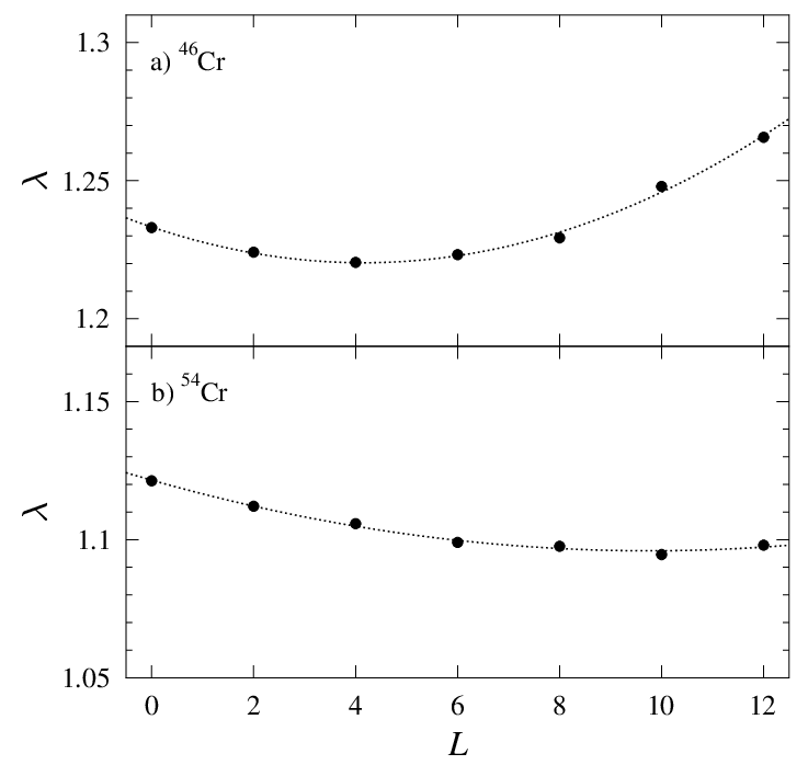
The dependence of can be fitted by a parabola
| (4) |
with the values (1.09596), (), and (9.7575) for 46Cr (54Cr). The deviation between the parabolic fit in Eq. (4) and the values in Tables 1 and 2 is typically of the order of 0.001 or below, corresponding to energy shifts of less than 100 keV. Thus, the experimental excitation energies of the yrast bands in 46Cr and 54Cr can be nicely reproduced in the folding potential model in combination with a three-parameter parabolic fit for the potential strength parameter .
The experimental and calculated level schemes of 46Cr and 54Cr are shown in Figs. 3 and 4. The folding potential with constant strength ( adjusted to the ground states) shows a compressed rotational spectrum, in particular for states with small . A perfect reproduction of the excitation energies is obtained using the slightly -dependent strength parameter in Eq. (4). The potential by S&M describes the excitation energies, too.


For completeness it has to be noted that the reproduction of excitation energies (as shown in Figs. 3 and 4) is not trivial. Usual Woods-Saxon potentials show the trend of spectral inversion, i.e. excited states with are located below the ground state (e.g., [23]). Using typical parameters like fm and fm for 46Cr (54Cr), the first state is found at MeV ( MeV), and the state appears at MeV ( MeV). The situation becomes even worse as soon as Woods-Saxon parameters are chosen which were adjusted to elastic scattering. E.g., the geometry of the widely used potential by McFadden and Satchler [42] ( fm, fm) leads to excitation energies of the state of MeV ( MeV) for 46Cr (54Cr). Thus, results from usual Woods-Saxon potentials are not included in Figs. 3 and 4.
As soon as the potential strength is determined by adjustment of the strength
parameter , the corresponding wave functions can be calculated
by numerical solution of the Schrödinger equation. Reduced widths
and , intercluster separations
, and transition strengths result directly
from these wave functions (similar to S&M). Qualitatively, the general
findings of S&M are reproduced in the present study:
() The intercluster separation decreases slightly with
increasing angular momentum .
() The reduced widths and
decrease significantly with increasing .
() -clustering is more pronounced in 46Cr compared to
54Cr.
Similar results have been obtained in earlier studies for the neighboring
nucleus 44Ti and also for heavier nuclei (e.g.,
[43, 20, 44, 45]).
However, there are also some differences between the work of S&M and the present study. The intercluster separations are slightly larger in the present double-folding model. This holds in particular for states with small angular momentum where smaller values in S&M result from the Gaussian dip at small radii. In the present work the reduced widths are about 20% higher for states with low in 46Cr and almost a factor of two higher for 54Cr. transition strengths are also slightly higher (of the order of 10%) in the present study. Furthermore, it should be pointed out that the calculated transition strengths agree reasonably well with the experimental data (whenever available). Similar to the work of S&M, no effective charges are required here.
The intercluster separations require a special discussion. Typically, strong -cluster states are characterized by large intercluster separations (as also found by S&M). The present results in Tables 1 and 2 indicate that the are close and even slightly larger for 54Cr with its smaller reduced widths . However, as soon as the radii are normalized to the radius of the compound radius by , these reduced radii show the expected behavior and are larger for 46Cr. So I do not provide a detailed discussion on the intercluster radii because the results are not unique.
4 Analysis of elastic scattering
Finally, it is interesting to test the -cluster potentials for 50Ti(,)50Ti elastic scattering. Here I first focus on the angular distribution at MeV by Gubler et al. [33] which is available from the EXFOR database [46]. This angular distribution covers the full angular range from about to in the center-of-mass system and is thus well-suited for the determination of the optical potential. In addition, it has been shown for the neighboring 40Ca(,)40Ca scattering that the optical potential at low energies ( MeV) is very close to the -cluster potential which describes the 44Ti ground state band [18]. For completeness, angular distributions at 104 MeV [35] and 140 MeV [34] will also be analyzed. Unfortunately, elastic (,) scattering data are not available for the radioactive 42Ti nucleus.
As a first step of the optical model analysis of the 50Ti(,)50Ti elastic scattering angular distribution at 25 MeV, a phase shift fit (according to the technique of [47]) was performed, and it is found that the experimental angular distribution can be very well reproduced (see Fig. 5). Next, optical model fits have been performed with the -cluster potential as a starting point for the real part. In extension to the real potential in Eq. (2), a phenomenological potential in the imaginary part was used which is taken as the sum of volume and surface Woods-Saxon potentials:
| (5) |
with
| (6) |
and . The depths , , radii , , and diffusenesses , of the volume and surface part have been adjusted to the experimental angular distribution. Note that in the above definition the maximum depth of the surface part is .
A further small modification of the width of the folding potential in the real part in Eqs. (1) and (2) is introduced:
| (7) |
Here is a width parameter which should remain very close to unity (see further discussion below).
Various fits for the angular distribution at 25 MeV [33] are shown in Fig. 5. The parameters of all fits are listed in Tables 3 and 4.

| type | |||||||||
|---|---|---|---|---|---|---|---|---|---|
| (MeV) | (MeV fm3) | (fm) | (MeV fm3) | (fm) | (mb) | ||||
| 25.0 | fold. | exp. [30] | 1.246 | 324.9 | 4.305 | 63.5 | 4.580 | 1395 | |
| 25.0 | fold. | exp. [30] | 1.247 | 345.1 | 4.391 | 66.8 | 4.409 | 1337 | |
| 25.0 | fold. | theo. [32] | 1.294 | 341.8 | 4.388 | 67.4 | 4.448 | 1343 | |
| 25.0 | S&M | 301.1 | 4.323 | 68.5 | 4.646 | 1404 | |||
| 104.0 | fold. | theo. [32] | 1.249 | 289.8 | 4.377 | 88.2 | 5.037 | 1557 | |
| 104.0 | S&M | 301.1 | 4.323 | 92.2 | 4.754 | 1413 | |||
| 140.0 | fold. | theo. [32] | 1.237 | 290.3 | 4.505 | 94.9 | 5.275 | 1687 | |
| 140.0 | S&M (V1) | 301.1 | 4.323 | 239.4 | 4.649 | 1638 | |||
| 140.0 | S&M (V2) | 301.1 | 4.323 | 115.0 | 5.302 | 1805 |
| type | ||||||||
| (MeV) | (MeV) | (fm) | (fm) | (MeV) | (fm) | (fm) | ||
| 25.0 | fold. | exp. [30] | 1.385 | 0.263 | 1.876 | 0.591 | ||
| 25.0 | fold. | exp. [30] | 1.355 | 0.191 | 1.741 | 0.391 | ||
| 25.0 | fold. | theo. [32] | 1.353 | 0.185 | 1.746 | 0.406 | ||
| 25.0 | S&M | 1.386 | 0.220 | 1.958 | 0.457 | |||
| 104.0 | fold. | theo. [32] | 1.400 | 0.547 | 1.631 | 0.608 | ||
| 104.0 | S&M | 1.458 | 0.368 | 1.691 | 0.459 | |||
| 140.0 | fold. | theo. [32] | 1.296 | 0.519 | 1.544 | 0.765 | ||
| 140.0 | S&M (V1) | 1.413 | 0.204 | 1.830 | 0.320 | |||
| 140.0 | S&M (V2) | 2.106 | 0.715 | 1.793 | 0.783 | |||
| aNote that the sum of volume and surface imaginary potential does not change its sign. | ||||||||
The folding potential which is based on the experimental charge density distribution of 50Ti does not exactly match the diffraction pattern in the forward region. The maxima and minima of the theoretical angular distribution are shifted towards larger angles; this corresponds to a potential which is slightly too narrow. After scaling the radial dependence of the real potential by a factor of a much better fit is obtained (for technical details, see [29]). Such a behavior is not surprising for 50Ti with because the neutron distribution should have a larger radial extent than the proton (charge) distribution. Evidence for a larger radial extent of the neutron distribution of 50Ti was also derived from scattering at higher energies [48].
Fortunately it turns out that the folding potential which is calculated from the theoretical density distribution of 50Ti (as provided in TALYS) is able to reproduce the experimental angular distribution without a significant radial scaling (the best fit is obtained using a scaling parameter of , i.e., very close to unity). This confirms the reliability of the theoretical density distribution of 50Ti which is consequently used throughout this paper.
The best-fit potential shows a real volume integral of MeV fm3 and fm; the imaginary part has MeV fm3 and fm. (As usual, the negative sign of the volume integrals is negelected in the discussion of and .) The real volume integral from elastic scattering is close to the results from scattering on neighboring nuclei [18] but significantly larger than the values for the -cluster states which are around MeV fm3 (see Table 2). For very pronounced -cluster nuclei like 44Ti or 20Ne such deviations are neither expected nor found [18, 14], and thus this deviation for 54Cr may be interpreted that 54Cr is not a very pure 50Ti cluster. This interpretation is in agreement with the smaller reduced widths which are found for 54Cr (in comparison to 46Cr and 44Ti).
As the potential by S&M has been optimized for the description of -cluster states with low MeV fm3, it is not surprising that this potential cannot reproduce the 50Ti(,)50Ti angular distribution with similar quality as the double-folding potentials. Furthermore, fm of the S&M potential is also lower than the best-fit values around 4.39 fm by about 2%.
At higher energies the differences between the folding potential and the potential by S&M become even more obvious. Indeed, the volume integral and the radius of the S&M potential are close to the results of Roberson et al. at MeV [34]. However, angular distributions at higher energies are not only sensitive to the potential at the nuclear surface but depend on the shape of the potential in a wider radial range. In the following I analyze the angular distributions at 140 MeV by Roberson et al. [34] and at 104 MeV by Pesl et al. [35]. Unfortunately, the 140 MeV data (as provided by EXFOR) had to be re-read from Fig. 1 of [34]; this leads to increased uncertainties and lower reliability of the extracted parameters. As no uncertainties are provided in EXFOR, a fixed uncertainty of 5% was assumed for the fitting procedure. Furthermore, the angular range of the 140 MeV data is limited to about , and the number of data points (51) is not very high. The angular distribution at 104 MeV [35] covers a larger angular range up to , consists of a factor of three more data points, and is available numerically (including uncertainties) from the internal report KFK-3242 [49].
The 140 MeV data can be nicely reproduced by the folding potential (see Fig. 6). The resulting volume integrals and are close to the results obtained for neighboring nuclei [18]: decreases with increasing energy, and approaches a saturation value of about 100 MeV fm3. An early study with folding potentials has also determined similar volume integrals [50]. Thus, the present analysis mainly confirms that the chosen theoretical density of 50Ti in combination with the DDM3Y interaction is appropriate.

Keeping a fixed real part from S&M and adjusting only the imaginary potential leads to a significantly worse reproduction of the experimental angular distribution. The best fit shows a strongly oscillating angular distribution at backward angles, correlated with very different imaginary volume integral . It is obvious from Fig. 6 that the strongly oscillating backward cross sections are not sufficiently constrained by the few experimental data points above about . A further local minimum in can be found with reasonable volume integrals (V2 in Fig. 6 and Tables 3 and 4); however, this results in a relatively poor reproduction of the experimental data at forward angles.
Also the angular distribution at 104 MeV [35] is very well reproduced by the folding potential (see Fig. 7). Interestingly, the width parameter for the 104 MeV data is very close (within 0.7%) to the 25 MeV fit. For the 140 MeV data the resulting width parameter was about 2% higher. This finding may have been affected from the uncertainties of the re-digitization of the 140 MeV data and the missing experimental uncertainties.

The fit with the fixed S&M real part results in volume integrals which are very close to the folding potential results. It is not surprising that the fixed S&M real part cannot reproduce the experimental angular distribution with the accuracy as the folding potential with two adjustbale parameters (strength and width ). But even if the same scaling parameters ( and ) are applied to the S&M potential, it is not possible to reproduce the angular distribution with a similar quality as the folding potential.
Summarizing the above analysis of elastic scattering angular distributions, it can be stated that the folding potential is able to describe the angular distributions over a wide energy range with smoothly varying parameters. The width parameter remains very close to unity using a theoretical density of 50Ti whereas a folding potential derived from the experimental charge distribution requires a radial scaling of about 2%.
The potential of S&M is close to the folding potential whose parameters have been adjusted to elastic scattering angular distributions. This is a quite noticeable finding because the S&M potential was optimized only for the reproduction of excitation energies of 54Cr. Without any further adjustment of the real part, the S&M potential cannot reach the same accuracy in the reproduction of the angular distributions, but it still provides a reasonable description of the experimental data at 25 MeV and 104 MeV.
5 Summary and conclusions
-cluster states in 46Cr and 54Cr are studied on the basis of a double-folding potential. A minor and smooth variation of the potential strength is found for the states under study in 46Cr and 54Cr. Reduced widths, intercluster separations, and transition strengths are close to the results of a recent study by Souza and Miyake [1] using a specially shaped potential, and the calculated transition strengths show reasonable agreement with the experimental values without effective charges. The present study confirms the significant -cluster properties of 46Cr and smaller reduced widths for 54Cr. Furthermore, it is found that the specially shaped potential by S&M is close to the double-folding potential of the present study (except at very small radii).
The application of the double-folding potential to elastic 50Ti(,)50Ti scattering provides excellent fits for the angular distributions over a wide energy range from 25 MeV to 140 MeV. The derived parameters show that the underlying 50Ti density should be preferentially taken from theory. The potential which is calculated from the experimental charge density distribution, turns out to be too narrow by about 2%, thus indicating a larger radial extent of the neutron distribution in 50Ti.
Acknowledgments
I thank M. A. Souza and H. Miyake for providing their results amd for encouraging discussions. This work was supported by OTKA (K108459 and K120666).
References
- (1) M. A. Souza and H. Miyake, Europ. Phys. J. A 53:146 (2017)
- (2) H. Horiuchi, K. Ikeda, K. Katō, Prog. Theor. Phys. Suppl. 192, 1 (2012).
- (3) S. Ohkubo, M. Fujiwara, P. E. Hodgson, Prog. Theor. Phys. Suppl. 132, 1 (1998).
- (4) F. Michel, S. Ohkubo, G. Reidemeister, Prog. Theor. Phys. Suppl. 132, 7 (1998).
- (5) T. Yamaya, K. Katori, M. Fujiwara, S. Kato, S. Ohkubo, Prog. Theor. Phys. Suppl. 132, 73 (1998).
- (6) T. Sakuda and S. Ohkubo, Prog. Theor. Phys. Suppl. 132, 103 (1998).
- (7) E. Uegaki, Prog. Theor. Phys. Suppl. 132, 135 (1998).
- (8) M. Hasegawa, Prog. Theor. Phys. Suppl. 132, 177 (1998).
- (9) S. Koh, Prog. Theor. Phys. Suppl. 132, 197 (1998).
- (10) A. Tohsaki, Prog. Theor. Phys. Suppl. 132, 213 (1998).
- (11) P. Descouvemont, Nucl. Phys. A709, 275 (2002).
- (12) T. Sakuda and S. Ohkubo, Nucl. Phys. A712, 59 (2002).
- (13) P. Mohr, H. Abele, V. Kölle, G. Staudt, H. Obrhummer, H. Krauss, Z. Phys. A 349, 339 (1993).
- (14) H. Abele and G. Staudt, Phys. Rev. C 47, 742 (1993).
- (15) S. Wilmes, V. Wilmes, G. Staudt, P. Mohr, J. W. Hammer, Phys. Rev. C 66, 065802 (2002).
- (16) P. Mohr, Phys. Rev. C 72, 035803 (2005).
- (17) P. Mohr, C. Angulo, P. Descouvemont, H. Utsunomiya, Europ. Phys. J. A 27, s01, 75 (2006).
- (18) U. Atzrott, P. Mohr, H. Abele, C. Hillenmayer, and G. Staudt, Phys. Rev. C 53, 1336 (1996).
- (19) F. Hoyler, P. Mohr, G. Staudt, Phys. Rev. C 50, 2631 (1994).
- (20) S. Ohkubo, Phys. Rev. Lett. 74, 2176 (1995).
- (21) P. Mohr, Europ. Phys. J. A 31, 23 (2007).
- (22) S. Ohkubo, Int. J. Mod. Phys. A 14, 2035 (2009).
- (23) P. Mohr, The Open Nuclear and Particle Physics Journal 1, 1 (2008).
- (24) P. Mohr, Phys. Rev. C 61, 045802 (2000).
- (25) Chang Xu and Zhongzhou Ren, Phys. Rev. C 73, 041301(R) (2006).
- (26) P. Mohr, Phys. Rev. C 95, 011302(R) (2017).
- (27) G. R. Satchler and W. G. Love, Phys. Rep. 55, 183 (1979).
- (28) A. M. Kobos, B. A. Brown, R. Lindsay, and G. R. Satchler, Nucl. Phys. A425, 205 (1984).
- (29) P. Mohr, G. G. Kiss, Zs. Fülöp, D. Galaviz, Gy. Gyürky, E. Somorjai, At. Data Nucl. Data Tables 99, 651 (2013).
- (30) H. de Vries, C. W. de Jager, and C. de Vries, Atomic Data and Nuclear Data Tables 36, 495 (1987).
- (31) K. Tsukuda et al., Phys. Rev. Lett. 118, 262501 (2017).
- (32) A. J. Koning, S. Hilaire, S. Goriely, computer code TALYS, version 1.8, http://www.talys.eu; A. J. Koning, S. Hilaire, and M. C. Duijvestijn, AIP Conf. Proc. 769, 1154 (2005).
- (33) H. P. Gubler, U. Kiebele, H. O. Meyer, G. R. Plattner, I. Sick, Nucl. Phys. A351, 29 (1981).
- (34) P. L. Roberson, D. A. Goldberg, N. S. Wall, L. W. Woo, H. L. Chen, Phys. Rev. Lett. 42, 54 (1978).
- (35) R. Pesl, H. J. Gils, H. Rebel, E. Friedman, J. Buschmann, H. Klewe-Nebenius, S. Zagromski, Z. Phys. A 313, 111 (1983).
- (36) Online database ENSDF, available at www.nndc.bnl.gov/ensdf; based on [37, 38].
- (37) S.-C. Wu, Nucl. Data Sheets 91, 1 (2000).
- (38) Yang Dong and Huo Junde, Nucl. Data Sheets 121, 1 (2014).
- (39) B. Buck, A. C. Merchant, S. M. Perez, Phys. Rev. C 51, 559 (1995).
- (40) F. Michel, J Albinski, P. Belery, Th. Delbar, Gh. Grégoire, B. Tasiaux, G. Reidemeister, Phys. Rev. C 28, 1904 (1983).
- (41) F. Michel, G. Reidemeister, S. Ohkubo, Phys. Rev. C 61, 041601(R) (2000).
- (42) L. McFadden and G. R. Satchler, Nucl. Phys. 84, 177 (1966).
- (43) M. A. Souza and H. Miyake, Phys. Rev. C 91, 034320 (2015).
- (44) F. Michel, G. Reidemeister, S. Ohkubo, Phys. Rev. C 37, 292 (1988).
- (45) B. Buck, C. B. Dover, J. P. Vary, Phys. Rev. C 11, 1803 (1975).
- (46) N. Otuka et al., Nucl. Data Sheets 120, 272 (2014); EXFOR database available online at http://www-nds.iaea.org/exfor/exfor.htm.
- (47) V. Chisté, R. Lichtenthäler, A. C. C. Villari, L. C. Gomes, Phys. Rev. C 54, 784 (1996).
- (48) H. J. Gils, H. Rebel, E. Friedman, Phys. Rev. C 29, 1295 (1984).
- (49) R. Pesl, internal report KFK-3242, Kernforschungszentrum Karlsruhe (1982); available at https://publikationen.bibliothek.kit.edu/270016791.
- (50) A. M. Kobos, B. A. Brown, P. E. Hodgson, G. R. Satchler, A. Budzanowski, Nucl. Phys. A384, 65 (1982).