A New Spectral Clustering Algorithm
Abstract
We present a new clustering algorithm that is based on searching for natural gaps in the components of the lowest energy eigenvectors of the Laplacian of a graph. In comparing the performance of the proposed method with a set of other popular methods (KMEANS, spectral-KMEANS, and an agglomerative method) in the context of the Lancichinetti-Fortunato-Radicchi (LFR) Benchmark for undirected weighted overlapping networks, we find that the new method outperforms the other spectral methods considered in certain parameter regimes. Finally, in an application to climate data involving one of the most important modes of interannual climate variability, the El Niño Southern Oscillation phenomenon, we demonstrate the ability of the new algorithm to readily identify different flavors of the phenomenon.
Index Terms:
Clustering, eigenvectors, machine learningI Introduction
Clustering is an unsupervised learning technique used to identify natural subgroups of a set of data wherein the members of a subgroup share certain properties. On representing the set of data as a graph, clustering methods group vertices of the graph into clusters based on the edge structure of the graph (23, e.g., see). We note here that the edge structure itself may be derived purely from interactions between vertices11 1 and in which context clustering is commonly referred to as community-detection, e.g., as in a social network, or based on a measure of similarity between the vertices themselves, or some combination of the two. Needless to mention, clustering methods find use in an extremely wide range of disciplines (e.g., neuroscience [7], social networks [17], computer vision [8], and digital forensic analysis [4]). Indeed most modes of climate variability are typically first identified by applying clustering methods to climatological data sets (e.g., 14, 3, 29, 10, 26, and others).
Since approaches to clustering are extremely varied, we do not attempt even a brief overview of such methods. For that the reader is referred to reviews such as [23]. Instead, we shift focus directly to the new algorithm after briefly considering common aspects of spectral approaches. In this article, we propose a spectral clustering algorithm based on direct analysis of the magnitudes of components of the eigenvectors (of the Laplacian matrix; see next section) with smallest eigenvalues. We call this algorithm spectral maximum gap method (SP-MGM). We compare the performance of this algorithm with popular clustering algorithms including k-means (KMEAN), more typical spectral clustering based on running kmeans on eigenvectors (SP-KMEANS), and agglomerative clustering (AGG). To determine the performance of these algorithms, we rely on a series of LFR benchmark graphs [13]. Notably, it is seen that on a certain series of these graphs with varying size, average degree, and weight mixing parameter, our algorithm consistently outperform these other methods. Following our benchmark analysis, we apply SP-MGM to a collection of monthly averaged sea surface temperatures in the Niño 3.4 region of the Pacific Ocean. We demonstrate that our method correctly and readily identifies the various flavors of El Niño and La Niña events.
II Spectral Clustering Algorithms
Spectral clustering algorithms rely on using spectral characteristics of the Laplacian of a (weighted) graph to partition the vertices of the graph into natural clusters. Here, the Laplacian can refer to the normalized Laplacian, the non-normalized Laplacian, or even stranger entities like the -Laplacian [2]. The use of spectral characteristics to identify clusters in a graph may be justified in numerous ways, such as by considering random walks, minimal cuts, or block matrix diagonalization. For a recent survey on spectral clustering methods, the reader is referred to [18]; for an introduction to spectral clustering itself, see, e.g., [31].
To present a brief and intuitive description of spectral clustering methods, we consider the eigenvectors of the Laplacian of a disconnected graph. Let be a graph with adjacence matrix and degree matrix (the diagonal matrix whose nonzero entries are the degrees of the vertices of ). Then the (non-normalized) Laplacian of is defined as . The matrix is positive semidefinite, and the kernel has a basis spanned by the indicator functions of the connected components of . In particular, if is disconnected then the connected components of may be deduced from the kernel of .
Clusters in a graph are intuitively regions in where the vertices are connected by edges with strong weights, relative to the weights of edges going between clusters. For this reason, the Laplacian of the graph should be very close to the Laplacian of the disconnected graph formed from by deleting intercluster edges. This means that the eigenvalues of will correspond approximately to the eigenvalues of . Since is positive semidefinite, the smallest eigenvalue of is zero. Therefore the eigenvectors of the smallest eigenvalues of should be small perturbations of vectors in the kernel of . Thus by analyzing the structure of the eigenvectors corresponding to the smallest handful of eigenvalues of , we should expect to retrieve information about the clusters of . It is exactly this idea that all spectral clustering algorithms exploit. Note that if is connected, then the kernel of consists of vectors whose entries are all identical, and therefore does not provide any information. For this reason, the kernel of is typically ignored in spectral clustering algorithms.
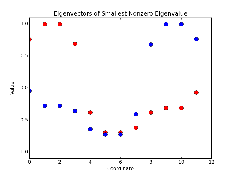
To further clarify this idea, consider the example of three cliques of size joined together by single bonds in general position, as in Figure 1(a).

The non-normalized Laplacian of this graph in block matrix form is
the Laplacian of a clique, , and the matrix whose only nonzero entry is and occurs in the bottom left corner. The eigenvalues of this matrix are and with multiplicity , and with multiplicity , and with multiplicity , where here . A basis for the for the eigenspace of the lowest nonzero eigenvalue is plotted in Figure 1(b). The stucture of these eigenvectors successfully reveals the presence of the three clusters.
In our algorithm, spectral clustering on a given data set occurs in three parts. We first create a similarity matrix describing the similarity or connectedness between each of our pieces of data. Secondly, we calculate the eigenvectors of the Laplacian of , and sort them in terms of the magnitudes of the associated eigenvalues. Lastly, we use some number of the eigenvectors with the smallest nonzero eigenvalues to calculate a natural partition of the vertices of the graph.
A similarity matrix for a collection of indexed data points is an symmetric matrix whose ’th entry is a nonnegative value measuring the similarity between the and ’th data values. It is assumed that larger values indicate more similar objects, and the diagonal elements are typically taken to be . Similarity matrices can be created out of data in a variety of ways. One popular method is to start with the distance between and (under some metric), and then define for , where here is a parameter.
The (symmetric) normalized Laplacian of is the graph Laplacian of the unique weighted graph whose weight matrix is . In particular, it is defined by
where here is a diagonal matrix whose entries are the sums of each of the column vectors of . The matrix is positive-semidefinite and will always have at least one eigenvector with eigenvalue , given by . However, assuming that the graph associated to is connected, this will be the only eigenvector with eigenvalue , up to constant multiples.
The smallest nonzero eigenvectors of encode clustering information for , and it is these eigenvectors which we wish to parse in the final step. The reason these eigenvectors contain clustering information can be made intuitive by the following argument. Clusters consist of regions in the graph with strong interconnectivity. Specifically, given a vertex in a cluster we would expect that on average the strength of its connection with other vertices in the same cluster should be much greater than the strength of its connection with vertices in other clusters. From this point of view, we can decompose the adjacency matrix as where is a block diagonal matrix whose blocks are formed by eliminating inter-cluster bonds, and where is relatively small compared to . In this case, the Laplacian of may be written as where is the Laplacian of and is small relative to . Consequently the eigenvectors of will be comparable ot the eigenvectors of . In particular the eigenvectors of correspond precisely with the eigenvectors of with small eigenvalues. Moreover, these eigenvectors describe the connected components of the graph of , and these are precisely the clusters of . In this way, using the eigenvectors of the smallest nonzero eigenvalues makes sense.
Where various clustering algorithms differ is in this third step, where the eigenvector data is used to calculate clusters. Before proposing our own clustering scheme, we will recount two common methods found in the literature, the simplest method SP-G1 and the most common method SP-KMEANS.
II-A SP-G1 clustering
The oldest and most basic algorithm is SP-G1, which decomposes the data into two clusters based on the entries of the eigenvector with the lowest nonzero eigenvalue [6][9]. Specifically, a theshold value needs to be chosen. Then the ’th data point is put into the first cluster if , and otherwise it is put into the second cluster. Of course, there are several natural choices for , including . Of course, more sophisticated methods for the choice of exist[25].
II-B SP-KMEANS
A more complicated and very reliable clustering algorithm instead uses eigenvectors of the smallest positive eigenvalues of the Laplacian of . These eigenvectors are used as the column vectors of an matrix . The matrix is then normalized so that each of the rows has norm , and the associated row vectors are viewed as points on the surface of a sphere in . Then by running KMEANS on these points, we return clusters of the data which partition the original graph [19][16]. The reliability and familiarity of this algorithm has lead to its popularity as one of the most common forms of spectral clustering, with implementations in both R and python [20][11].
II-C Spectral Maximum Gap Method (SP-MGM)
In the new SP-MGM algorithm we propose, the eigenvectors of the smallest positive eigenvalues of the Laplacian of are first calculated. Next, for each we create a new vector whose entries are the entries of in increasing order. Let and denote the entries of and , respectively. Differences between subsequent entries of represent “gaps" in .
We choose so that is the largest gap. Then we create a partition of by placing vertex in if , and placing vertex in otherwise. Finally, for each subset of we define a cluster
where here if or is empty, the associated intersection is interpreted to be . It is clear from the construction that forms a partition of .
The number of clusters in this partition is at least , but can be up to . However, in practice it is observed that many of the clusters are repeated, and the algorithm tends to find far fewer than clusters. In fact, the number of clusters created in this way tends to be close to the actual right number of clusters. This will be discussed further in the benchmark section below. Note that we experimented with both using the normalized and non-normalized Laplacian. We found that the non-normalized Laplacian performs better for the benchmark graphs that we considered. We note that a common and effective strategy in applying spectral methods to large data sets consists of adopting a hierarchical approach wherein spectral techniques are used on subsets of the data that are then recombined (15, 28, 24, 21, e.g., see).
II-C1 A mathematical justification of the new algorithm
We provide a mathematical justification of the SP-MGM algorithm by applying the theory of eigenvector permutations to the Laplacian of the graph . We provide full mathematical details in the appendix for the interested reader. However, we restrict ourselves to a brief description of the justification here so as to keep the narrative more generally accessible: First, we show mathematically that if consists of several well-defined clusters of size then
for all . Here and are spectral data which measure the quality of the clusters. Specifically, is the smallest nonzero eigenvalue of cluster and measures the connectivity of the cluster . For this reason, it is sometimes called the algebraic connectivity of the cluster . The number is the spectral radius of the Laplacian of the graph formed by deleting all of the intra-cluster edges in . In this way, it measures the strength of the inter-cluster connections. For a strongly clustered graph, it therefore makes sense that is small relative to for all . Further, if consists of several such clusters , then, we can mathematically guarantee that SP-MGM will correctly identify the clusters. Again, the reader is referred to the appendix for details.
III Benchmark Experiments
III-A LFR Benchmark
To test the quality of our clustering/community-detection algorithm, we choose to use the LFR benchmark. Benchmark graphs consist of randomly generated graphs with built-in network ties. The properties of the output graph are controlled by a series of parameters. The parameters we consider and vary are the total number of nodes , the average degree , the maximum degree , and the mixing parameter . Each node is given a degree based on a power law distribution. The minimum and maximum degrees in the network are chosen so that the mean from the power law distribution is . Nodes are assigned to clusters such that the (weighted) fraction of intercluster edges is . Source code for generating LFR Benchmark graphs is available at https://github.com/eXascaleInfolab/LFR-Benchmark_UndirWeightOvp.
Note also that each of the algorithms described above requires an important piece of user input: namely the number of clusters to look for. In practice, there are several ways of deciding how many clusters in a graph to look for, such as the elbow technique, the jump method, and silhouette analysis [12]. However, these seem outside the scope of the current paper. Instead, we supply each algorithm with the correct number of clusters to look for. The exception to this is SP-MGM, which does not take in a number of clusters to look for. Instead, it takes in a number of eigenmodes . However, in practice, the number of clusters it finds is , so we choose accordingly.
III-B The Quality of a Clustering Partition
After a clustering algorithm identifies one or more clusters in a graph, it is natural to want to identify the quality of the clusters. Are the vertices in a cluster naturally correlated in some fashion, or is the cluster only an artifact of the specified clustering algorithm? While there is no single criteria for reliably determining the quality of a cluster, there exist several metrics which may be used in combination to judge the reasonability of ones choice of clusters. For a comparison of several such metrics, see [1].
The LFR Benchmark produces a weighted graph, along with a predetermined true value for the neighborhoods. To determine the performance of each clustering algorithm we use two scoring metrics: the normalized mutual info score (NMI) and the adjusted rand score (ARS). In both metrics, the scores can range between and , with representing perfect cluster prediction and representing largely independent cluster prediction from the true clusters.
III-C Results
We will now compare the performance of our algorithm to the performance of a traditional spectral clustering SP-KMEANS, as well as traditional KMEANS and an agglomerative clustering algorithm. This collection of algorithms was chosen as a basis of comparison since they are notably diverse in their methodologies. At the same time, they are also popular enough to have been implemented in the widely-used python machine learning package scikit-learn [20]. While SP-KMEANS has already been described, the reader is referred to [22] for descriptions of KMEANS and the agglomerative methods.
III-C1 Variations in Mixing Parameter
The scores of clustering algorithms for the LFR benchmark on graphs with and nodes with varying mixing parameter are shown in Figures 2 and 3. From these figures, it is evident, and notably so, that SP-MGM consistently outperforms the other clustering algorithms considered for small networks over the entire range of the mixing parameter considered.


Next, we examined the performance of SP-MGM relative to the other algorithms considered while varying the average vertex degree, and the network size. Figure 4 shows the results when average vertex degree was varied. As the average network degree increased, all algorithms considered showed an increase in score. However, SP-MGM consistently out-performed the other algorithms considered. Furthermore, SP-MGM was the only algorithm to perform reasonably when the average vertex degree was small, and the mixing parameter was simultaneously low.
The scores of clustering algorithms for the LFR benchmark on graphs with and nodes with varying mixing number are shown in Figures 2 and 3. From these figures, it is evident, and notably so, that SP-MGM consistently outperforms the other clustering algorithms considered for small networks over the entire range of the mixing parameter considered.
For larger networks (not shown), SP-MGM performs comparably or better than the other algorithms considered when the algorithms are scoring high enough. In other words, when any of the algorithms perform well, SP-MGM performs well as well. We note here that when edges are distributed uniformly across the nodes, clusters are not well-defined, and as such, the computed clustering is likely not robust (and likely arbitrary) and therefore not meaningful or useful. Notably, for small values of the mixing parameter on small graphs, the prediction-skill of SP-MGM is far superior.
III-C2 Variations in Average Degree and Network Size
Next, we examined the performance of SP-MGM relative to the other algorithms considered while varying the average vertex degree, and the network size. Figure 4 shows the results when average vertex degree was varied. As the average network degree increased, all algorithms considered showed an increase in score. However, SP-MGM consistently out-performed the other algorithms considered. Furthermore, SP-MGM was the only algorithm to perform reasonably when the average vertex degree was small, and the mixing parameter was simultaneously low.
Figure 5 shows the results when the network size was varied. SP-MGM is seen to perform well over a range of network sizes, with only the agglomerative clustering algorithm out-performing it for larger graph sizes. We note, however, that the new algorithm tended to outperform its spectral counterpart SP-KMEAN over the full range of network sizes considered.
III-C3 The Number of Clusters SP-MGM Detects
From the description of the SP-MGM algorithm, it is seen that we need to specify only the number of eigenmodes to consider. For this reason, a priori the algorithm should be able to predict anywhere from and clusters, where here is the total number of vertices in the graph. However, in practice the algorithm almost always produces clusters, at least for all the test graphs examined in this paper. This result is quite surprising, since from an intuitive perspective one would suspect the number of clusters produced to be far more volatile. It seems like this is additional computational evidence that the “maximum gaps" we are computing must have a lot to do with the structure of the graphs themselves, closely tied to the clusters.
IV Clustering of SST data in El Niño 3.4

In this section we consider the application of the new clustering algorithm to a real world data set in the context of the climate system. Specifically we consider the El Niño Southern Oscillation (ENSO) since it is one of the most important modes of interannual variability of the climate system. It can be characterised in terms of the sea surface temperature anomaly occuring in a region of the equatorial Pacific Ocean. The ENSO temperature anomaly roughly fluctuates between three phases: a warm El Niño phase, a cold La Niña phase, and a neutral phase. The phases of ENSO are correlated with changes in precipitation in various regions around the globe, with strong correlations in coastal Pacific regions. As such, predictions of ENSO have high socio-economic value, Luckily, ENSO also happens to be one of the few modes of interannual variability that has a useful level of verified predictability.
IV-A Sea Surface Temperature Data
We use version 4 of the Extended Reconstructed Sea Surface Temperature (ERSST) dataset available at https://www.esrl.noaa.gov/psd/data/gridded/data.noaa.ersst.v4.html. The data has a spatial resolution of 2 degree, and while the monthly-averaged data that we use are available from 1854-present, we focus attention on data over the years 1955-2016, given lower uncertainties over this more recent (instrumented) period. For further description of the data, the reader is referred to https://www.ncdc.noaa.gov/data-access/marineocean-data/extended-reconstructed-sea-surface-temperature-ersst-v4.
IV-B El Niño Events

The average sea surface temperature is calculated using a -year average of the NOAA ERSST data starting Jan 1, 1950. SST anomaly is calulated relative to this mean [27].
We consider the data from ERSSTv4 in the Niño 3.4 region (the region between 170W and 120W longitude and between -5N and 5N latitude), as shown in Figure 6. El Niño events are classified by a persistent large average temperature anomaly in this region. Quantitatively, El Niño events are determined by the Oceanic Niño Index (ONI), which is a -month running mean of the SST anomaly spatially averaged over the Niño 3.4 region. A Niño event is characterized by ONI values greater than degrees C for at least three months in a row. The years of El Niño events between 1950 and 2000 may be seen from the graph in Figure (7) below.
IV-C Clustering Results

While ONI is a conventional and simple measure that is used to classify the state of ENSO, the phenomenon itself is more complicated. That is, although the ENSO phenomenon can be characterized as a low-dimensional dynamical phenomenon occuring in an infinite-dimensional dynamical system, it is unlikely to be fully or adequately characterized by just ONI. As such, we conduct a clustering analysis of the spatially-extended sea surface temperature anomaly (SSTA) dataset T(x, y, t) where t runs from years 1955 through 2016 and x and y correspond to the Niño 3.4 region described above. The data vector for each year itself is a 3-month average starting from November of the previous year.
In order to conduct cluster analysis, we next transform the SSTA dataset into a graph whose vertices are the yearly SSTA datapoints embedded in a high-dimensional space, the number of dimensions corresponding to the number of distinct spatial locations in the Niño 3.4 region. Next we consider an edge structure that reflects the mutual similarity of pairs of vertices. The resultant similarity matrix has the form for , where , and where the spatially-extended covariance matrix for the period considered. Note that is also sometimes called the precision matrix. For simplicity, we consider a diagonal form for that comprises the variances of the SSTA at each of the spatial locations in the Niño 3.4 region. The parameter toggles controls localization of the similarity matrix; we use .
In Figure 8, the nodes are colored-coded based on cluster-membership and the nodes are placed at the two-dimensional point corresponding to the year (x-axis) and ONI of that year (y-axis). Finally, the thickness of the edges reflect similarity between the pair of vertices they connect. In this figure, it is seen that there is good correlation between the clusters and the conventional ONI (y-axis). Thus, the new clustering algorithm SP-MGM is seen to successfully distinguish between El Niño , La Niña , and neutral events.
Next, it is seen that the SP-MGM clustering algorithm identifies distinct clusters and that cluster membership is not solely determined by ONI. Indeed, that there are different flavors of ENSO besides El Niño and La Niña is now widely recognized and how these different flavors influence climate in different regions is an active area of research. The cluster patterns we find are consistent, e.g., with the patterns found in [10] who use a neural-network based analysis in conjunction with other statistical distinguishability tests. We note, however, that there are significant differences in the data used by [10] in that they consider a six month average starting in September and a much more extensive region of the Pacific.
V Conclusions
In this paper, we presented a new spectral clustering algorithm which we call the Spectral-Maximum Gap Method SP-MGM. This algorithm is based on identifying gaps in the structure of eigenvectors. We then went on to provide a mathematical justification for the algorithm. While it would be interesting to see where this algorithm fits in a systematic comparison of spectral algorithms, such as in [30], such a comparison is outside the scope of the current paper. Further, as with other spectral schemes, this method can be applied to large datasets in conjunction with a hierarchical approach as in (15, 28, 24, 21, and others).
Next, we examined the performance of this algorithm in comparison to a few other popular algorithms using the LFR benchmark graphs. Results showed that the SP-MGM algorithm performs either comparbly or better than its counterparts in a variety of parameter regimes. We also demonstrated how SP-MGM may be used to automatically detect an appropriate number of clusters for a specified graph. Finally, we applied this algorithm to analyze and identify a variety of flavors of the El Niño Southern Oscillation using spatially extended sea surface temperature data.
Acknowledgement
This work was performed during one authors visit to CNLS at Los Alamos National Lab.
Eigenvector Perturbation
The eigenvalue perturbation problem is the problem of estimating the eigenvectors and eigenvalues of a perturbed matrix based on the eigenvalues of the matrix , where here is a small positive number which estimates the size of the perturbation. In such a case one should rightfully assume that the eigenvalues and eigenvectors of and are nearly the same. In this section, we briefly recount the idea of eigenvector perturbation analysis, deriving in particular the linear perturbation equations for the eigendata of a perturbed matrix. This equation specifically relates the eigenvectors of and for sufficiently small. Our exposition is loosely based on that found in the standard source [5]. However, standard perturbation analysis formulas seems to emphasize the reqirement that the eigenvalues of are distinct, whereas our brief derivation shows that this is not the case, as long as the formulas are appropriately adjusted. This is important for our application to graph theory, where we wish to be the Laplacian of a disconnected graph.
Assume that are symmetric matrices and let be an orthonormal eigenbasis for , with . Then the linear perturbation equation says that for all there exists an eigenvector of satisfying
| (1) |
Furthermore the eigenvalue of is given by
| (2) |
where here the braces denote the usual inner product on .
To prove the above two equations, we can use a standard but important linear algebra tool: the resolvent of a matrix. Given any matrix , the resolvent is a matrix-valued rational function on the complex plane, defined by . One useful property of the resolvent is that acts like a projection operator onto the eigenspaces of . Specifically, if is an eigenvalue of and is a closed contour in the complex plane, then for any constant vector , the integral
is an eigenvector of with eigenvalue , as long as it is nonzero.
Now since , a simple calculation shows
For each , let be an eigenvalue of closest to . Take to be a closed contour in the complex plane containing and , but no other (distinct) eigenvalue of or . Then we know that
will be an eigenvector with eigenvalue . However, using our expression for we see that
Therefore by Cauchy’s residue theorem
This proves Equation 1. To get the associated eigenvalue , we can use the fact that
From our expression for , we have and . Thus
This proves Equation 2.
Mathematical Justification for SP-MGM
Let be a graph with vertices and let be the natural subclusters of . To show mathematically how SP-MGM detects the clusters from the graph , we will consider two subgraphs of , which we will call and , and which will be formed by deleting the intercluster bonds and intracluster bonds of , respectively. Also to simplify the notation, throughout this section we will think about the Laplacian of as acting not on , but rather on the space of real-valued functions on . For this reason, we will switch from talking about eigenvectors to talking about eigenfunctions. We will denote the Laplacians of , and as , and . Clearly .
To better understand why SP-MGM should work well, we need to consider in more detail the eigen-structure of the Laplacian of . The eigenfunctions of clearly restrict to each cluster to an eigenfunction on . Each cluster is connected, and therefore has a kernel spanned by its indicator function. Thus an orthonormal basis for the kernel of is given by
for . More generally, let be the eigenvalues of . Then the are also eigenvalues of and there exists an orthonormal eigenbasis for such that has eigenvalue and is supported on . By definition, .
Assuming that the clusters are really, honestly clusters and not just part of some artificial partition of , we should expect the spectral radius of to be small compared to the spectral radius of . Then the eigendata of and will be related via the eigenvector perturbation theory discussed above. Each of the will correspond to an eigenfunction of the matrix via this perturbation theory, and the associated eigenvalues should be expected to be the smallest eigenvalues of the matrix . Moreover, this eigenvalue perturbation theory gives us an estimate of relative to . If we can show that
then the location of the maximum gap in and the location of the maximum gap in must be the same! In this case, SP-MGM is guaranteed to identify a partition which correctly separates one of the clusters from the others.
From our eigenvalue perturbation theory, we know that for
to order , where . Since is supported on and sends to a function supported on the complement of , we find that to order
Thus we arrive at the conclusion that if is small and for all we have
Then SP-MGM will correctly identify the desired clusters.
References
- [1] Hélio Almeida, Dorgival Guedes, Wagner Meira, and Mohammed J Zaki. Is there a best quality metric for graph clusters? In Joint European Conference on Machine Learning and Knowledge Discovery in Databases, pages 44–59. Springer, 2011.
- [2] Thomas Bühler and Matthias Hein. Spectral clustering based on the graph p-laplacian. In Proceedings of the 26th Annual International Conference on Machine Learning, pages 81–88. ACM, 2009.
- [3] João Corte-Real, Budong Qian, and Hong Xu. Regional climate change in portugal: precipitation variability associated with large-scale atmospheric circulation. International Journal of Climatology, 18(6):619–635, 1998.
- [4] Sergio Decherchi, Simone Tacconi, Judith Redi, Alessio Leoncini, Fabio Sangiacomo, and Rodolfo Zunino. Text clustering for digital forensics analysis. Computational Intelligence in Security for Information Systems, pages 29–36, 2009.
- [5] Demmel. Applied numerical linear algebra. 1997.
- [6] Miroslav Fiedler. A property of eigenvectors of nonnegative symmetric matrices and its application to graph theory. Czechoslovak Mathematical Journal, 25(4):619–633, 1975.
- [7] Sally Galbraith, James A Daniel, and Bryce Vissel. A study of clustered data and approaches to its analysis. Journal of Neuroscience, 30(32):10601–10608, 2010.
- [8] Robert M Haralick and Linda G Shapiro. Image segmentation techniques. Computer vision, graphics, and image processing, 29(1):100–132, 1985.
- [9] Anil K Jain and Richard C Dubes. Algorithms for clustering data. Prentice-Hall, Inc., 1988.
- [10] Nathaniel C Johnson. How many enso flavors can we distinguish? Journal of Climate, 26(13):4816–4827, 2013.
- [11] Alexandros Karatzoglou, Alex Smola, Kurt Hornik, and Achim Zeileis. kernlab – an S4 package for kernel methods in R. Journal of Statistical Software, 11(9):1–20, 2004.
- [12] Trupti M Kodinariya and Prashant R Makwana. Review on determining number of cluster in k-means clustering. International Journal, 1(6):90–95, 2013.
- [13] Andrea Lancichinetti, Santo Fortunato, and Filippo Radicchi. Benchmark graphs for testing community detection algorithms. Physical review E, 78(4):046110, 2008.
- [14] Robert Lund and Bo Li. Revisiting climate region definitions via clustering. Journal of Climate, 22(7):1787–1800, 2009.
- [15] Ulrike V Luxburg, Olivier Bousquet, and Mikhail Belkin. Limits of spectral clustering. In Advances in neural information processing systems, pages 857–864, 2005.
- [16] Marina Meila and Jianbo Shi. Learning segmentation by random walks. In Advances in neural information processing systems, pages 873–879, 2001.
- [17] Nina Mishra, Robert Schreiber, Isabelle Stanton, and Robert E Tarjan. Clustering social networks. In WAW, volume 4863, pages 56–67. Springer, 2007.
- [18] Maria CV Nascimento and Andre CPLF De Carvalho. Spectral methods for graph clustering–a survey. European Journal of Operational Research, 211(2):221–231, 2011.
- [19] Andrew Y Ng, Michael I Jordan, and Yair Weiss. On spectral clustering: Analysis and an algorithm. In Advances in neural information processing systems, pages 849–856, 2002.
- [20] F. Pedregosa, G. Varoquaux, A. Gramfort, V. Michel, B. Thirion, O. Grisel, M. Blondel, P. Prettenhofer, R. Weiss, V. Dubourg, J. Vanderplas, A. Passos, D. Cournapeau, M. Brucher, M. Perrot, and E. Duchesnay. Scikit-learn: Machine learning in Python. Journal of Machine Learning Research, 12:2825–2830, 2011.
- [21] Diego H Peluffo-Ordónez, John A Lee, and Michel Verleysen. Short review of dimensionality reduction methods based on stochastic neighbour embedding. In Advances in Self-Organizing Maps and Learning Vector Quantization, pages 65–74. Springer, 2014.
- [22] Lior Rokach and Oded Maimon. The data mining and knowledge discovery handbook: A complete guide for researchers and practitioners, 2005.
- [23] Satu Elisa Schaeffer. Graph clustering. Computer science review, 1(1):27–64, 2007.
- [24] Theodoros Semertzidis, Dimitrios Rafailidis, Michael G Strintzis, and Petros Daras. Large-scale spectral clustering based on pairwise constraints. Information Processing & Management, 51(5):616–624, 2015.
- [25] Jianbo Shi and Jitendra Malik. Normalized cuts and image segmentation. IEEE Transactions on pattern analysis and machine intelligence, 22(8):888–905, 2000.
- [26] Karsten Steinhaeuser, Nitesh Chawla, and Auroop Ganguly. Comparing predictive power in climate data: Clustering matters. Advances in Spatial and Temporal Databases, pages 39–55, 2011.
- [27] Kevin E Trenberth. The definition of el nino. Bulletin of the American Meteorological Society, 78(12):2771–2777, 1997.
- [28] Frederick Tung, Alexander Wong, and David A Clausi. Enabling scalable spectral clustering for image segmentation. Pattern Recognition, 43(12):4069–4076, 2010.
- [29] Yurdanur Unal, Tayfun Kindap, and Mehmet Karaca. Redefining the climate zones of turkey using cluster analysis. International journal of climatology, 23(9):1045–1055, 2003.
- [30] Deepak Verma and Marina Meila. A comparison of spectral clustering algorithms. University of Washington Tech Rep UWCSE030501, 1:1–18, 2003.
- [31] Ulrike Von Luxburg. A tutorial on spectral clustering. Statistics and computing, 17(4):395–416, 2007.
![[Uncaptioned image]](1710.02756v1/wcasper.jpg) |
W.R. Casper received BS degrees in mathematics and physics, as well as an MS in mathematics from North Dakota State University in 2010. He later received a PhD in mathematics from the University of Washington, Seattle in 2017. He is currently a postdoctoral researcher in the Department of Mathematics at Louisiana State University in Baton Rouge. His research interests are diverse, and include integrable systems, algebraic geometry, noncommutative algebra, geophysical fluid dynamics, computational physics and machine learning. |
![[Uncaptioned image]](1710.02756v1/balu.png) |
Balu Nadiga is a scientist at the Los Alamos National Lab. With a specialization in fluid dynamics, he has worked on problems ranging from climate and ocean circulation to turbulence modeling and multiphase flows. His other interests include dynamical systems, uncertainty quantification and Bayesian analysis, and using machine learning for turbulence modeling. |