Search-based Motion Planning for Aggressive Flight in SE(3)

Before introducing the planning approach, we inspect the relation between polynomial trajectories and system dynamics. The position $\mathbf{x}=[x,y,z]^{\mathsf{T}}$ in $\mathbb{R}^{3}$ of the quadrotor can be defined as a differentially flat output as described in [13]. The associated velocity $\mathbf{v}$, acceleration $\mathbf{a}$ and jerk $\mathbf{j}$ can be obtained by taking derivatives with respect to time as $\dot{\mathbf{x}},\ddot{\mathbf{x}},\dddot{\mathbf{x}}$ respectively. The desired trajectory for the geometric SE(3) controller as described in [28] can be written as $\Phi(t)=[\mathbf{x}_{d}^{\mathsf{T}},\mathbf{v}_{d}^{\mathsf{T}},\mathbf{a}_{d}^{\mathsf{T}},\mathbf{j}_{d}^{\mathsf{T}}]^{\mathsf{T}}$. According to [29], we assume the force and angular velocity are our control inputs to the quadrotor. Ignoring feedback control errors, the desired mass-normalized force in the inertial frame can be obtained as

$$\mathbf{f}_{d}=\mathbf{a}_{d}+g\mathbf{z}_{w}$$

(1)

where $g$ is the gravitational acceleration and $\mathbf{z}_{w}=[0,0,1]^{\mathsf{T}}$ is the z-axis of the inertial world frame. Similar to [28], given a specific yaw $\psi$, the desired orientation in SO(3) can be written as $\mathbf{R}_{d}=[\mathbf{r}_{1},\mathbf{r}_{2},\mathbf{r}_{3}]$ where

$$\mathbf{r}_{3}=\mathbf{f}_{d}/\|\mathbf{f}_{d}\|,\quad\mathbf{r}_{1}=\frac{\mathbf{r}_{2c}\times\mathbf{r}_{3}}{\|\mathbf{r}_{2c}\times\mathbf{r}_{3}\|},\quad\mathbf{r}_{2}=\mathbf{r}_{3}\times\mathbf{r}_{1}$$

(2)

and

$$\mathbf{r}_{2c}=[-\sin{\psi},\cos{\psi},0]^{\mathsf{T}}$$

(3)

which is assumed to be not parallel to $\mathbf{r}_{3}$. The associated angular velocity in the inertial frame, $\dot{\mathbf{R}}_{d}=[\dot{\mathbf{r}}_{1},\dot{\mathbf{r}}_{2},\dot{\mathbf{r}}_{3}]$, can be calculated as

	$\displaystyle\dot{\mathbf{r}}_{3}$	$\displaystyle=\mathbf{r}_{3}\times\frac{\dot{\mathbf{f}}_{d}}{\|\mathbf{f}_{d}\|}\times\mathbf{r}_{3},$
	$\displaystyle\dot{\mathbf{r}}_{1}$	$\displaystyle=\mathbf{r}_{1}\times\frac{\dot{\mathbf{r}}_{2c}\times\mathbf{r}_{3}+\mathbf{r}_{2c}\times\dot{\mathbf{r}}_{3}}{\|\mathbf{r}_{2c}\times\mathbf{r}_{3}\|}\times\mathbf{r}_{1},$		(4)
	$\displaystyle\dot{\mathbf{r}}_{2}$	$\displaystyle=\dot{\mathbf{r}}_{3}\times\mathbf{r}_{1}+\mathbf{r}_{3}\times\dot{\mathbf{r}}_{1}$

where

$$\dot{\mathbf{r}}_{2c}=[-\cos{\psi},-\sin{\psi},0]^{\mathsf{T}}\dot{\psi},\;\dot{\mathbf{f}_{d}}=\mathbf{j}^{\mathsf{T}}_{d}$$

(5)

Therefore, the desired angular velocity $\mathbf{w}_{d}$ in body frame is obtained as:

$$[\mathbf{w}_{d}]_{\times}=\mathbf{R}^{\mathsf{T}}_{d}\dot{\mathbf{R}}_{d}$$

(6)

Once the desired force $\mathbf{f}_{d}$, orientation $\mathbf{R}_{d}$ and angular velocity $\mathbf{w}_{d}$ are defined, it is straightforward to compute the desired control inputs for the quadrotor system. Notice that: 1) orientation is algebraically related to the desired acceleration and gravity and 2) angular velocity is algebraically related to the desired jerk.

As mentioned in the previous section, the desired trajectory can be defined as

$$\Phi(t):=[\mathbf{x}^{\mathsf{T}},\dot{\mathbf{x}}^{\mathsf{T}},\ddot{\mathbf{x}}^{\mathsf{T}},\dddot{\mathbf{x}}^{\mathsf{T}}]^{\mathsf{T}}=[\mathbf{x}^{\mathsf{T}},\mathbf{v}^{\mathsf{T}},\mathbf{a}^{\mathsf{T}},\mathbf{j}^{\mathsf{T}}]^{\mathsf{T}}$$

(7)

and each component of $\Phi(t)$ can be represented by a polynomial parameterized in time $t$. Position can be defined as

$$\mathbf{x}(t):=\sum_{k=0}^{K}d_{k}\frac{t^{k}}{k!}=d_{K}\frac{t^{K}}{K!}+\ldots+d_{1}t+d_{0}$$

(8)

where $d_{k}\in\mathbb{R}^{3}$ are the coefficients. The corresponding velocity, acceleration and jerk can be obtained by taking the derivative of (8). A polynomial trajectory from one state to the other within a specified time duration is called a motion primitive. Our approach uses primitives generated as the solutions to an optimal control problem [12] to build a graph from an initial state to a goal state and search for the optimal sequence of primitives. Technical details and proof of optimality can be found in our previous work [12]. In this paper, we give the explicit solution for generating the optimal trajectory using jerk as the control input.

We define the state

$$\mathbf{s}(t):=[\mathbf{x}(t)^{\mathsf{T}},\dot{\mathbf{x}}(t)^{\mathsf{T}},\ddot{\mathbf{x}}(t)^{\mathsf{T}}]^{\mathsf{T}}=[\mathbf{p}^{\mathsf{T}},\mathbf{v}^{\mathsf{T}},\mathbf{a}^{\mathsf{T}}]^{\mathsf{T}}$$

(9)

as a subset of the trajectory $\Phi(t)$ that excludes the jerk. From an initial state $\mathbf{s}_{0}=[\mathbf{p}_{0}^{\mathsf{T}},\mathbf{v}_{0}^{\mathsf{T}},\mathbf{a}_{0}^{\mathsf{T}}]^{\mathsf{T}}$, we apply a constant jerk input $\mathbf{u}_{m}$ from a pre-defined control set $\mathcal{U}_{M}$ for a short duration $\tau>0$. The resulting curve between $\mathbf{s}_{0}$ and the end state is a motion primitive such that for $t\in[0,\tau]$ the system state $\mathbf{s}(t)$ can be written as

$$\mathbf{s}(t)=F(\mathbf{u}_{m},\mathbf{s}_{0},t):=\begin{bmatrix}\mathbf{u}_{m}\frac{t^{3}}{6}+\mathbf{a}_{0}\frac{t^{2}}{2}+\mathbf{v}_{0}t+\mathbf{p}_{0}\\ \mathbf{u}_{m}\frac{t^{2}}{2}+\mathbf{a}_{0}t+\mathbf{v}_{0}\\ \mathbf{u}_{m}t+\mathbf{a}_{0}\end{bmatrix}$$

(10)

It has been shown in [21] and [12] that $F(\cdot)$ provides the minimum jerk trajectory between $\mathbf{s}_{0}$ and $\mathbf{s}(\tau)$.

The finite control input set $\mathcal{U}_{M}$ and duration $\tau$ define a graph $\mathcal{G}(\mathcal{S},\mathcal{E})$, where $\mathcal{S}$ is the set of reachable states in $\mathbb{R}^{9}$ and $\mathcal{E}$ is the set of edges connecting those states. The states in $\mathcal{S}$ are generated by applying each element of $\mathcal{U}_{M}$ at each state iteratively, and each element in $\mathcal{E}$ is a primitive as defined in (10). A breadth-first-search (BFS) of a finite horizon leads to the graphs shown in Fig. 2.

We are interested in finding a trajectory from $\mathbf{s}_{0}$ to $\mathbf{s}_{g}$ that is optimal in terms of total control effort $J$ and time $T$ taken to reach the goal. According to [12], a desired optimal trajectory is obtained as

$$\begin{gathered}\Phi^{*}(t)=\mathop{\arg\min}\limits_{\Phi(t)}J+\rho T=\mathop{\arg\min}\limits_{\Phi(t)}\int_{0}^{T}\|\mathbf{j}\|^{2}+\rho T\\ \begin{aligned} \text{s.t.}\;&\mathbf{s}_{0}\leftarrow\Phi(0),\;\mathbf{s}_{g}\leftarrow\Phi(T)\\ \end{aligned}\end{gathered}$$

(11)

where $\rho$ is the weight that decides the trade-off between effort and time.

For the primitive defined in (10), $J=\|\mathbf{u}_{m}\|^{2}\tau$ and $T=\tau$. Thus, the cost of a primitive of applying $\mathbf{u}_{m}$ from state $\mathbf{s}_{n}\in\mathcal{S}$ is defined as

$$C(\mathbf{s}_{n},\mathbf{u}_{m})=C(\mathbf{u}_{m})=(\|\mathbf{u}_{m}\|^{2}+\rho)\tau$$

(12)

The cost of the individual primitive is independent of the current state and only depends on the set $\mathcal{U}_{m}$ and $\tau$. In addition, it can be shown by Pontryagin’ minimum principle that (10) is the optimal solution of (11). Details of the proof can be found in [12]. Therefore, search for an optimal trajectory of (11) is equivalent to find the optimal solution to the following deterministic shortest path problem:

We are able to solve this problem through a graph search algorithm like A*. The optimal trajectory $\Phi^{*}(t)$ can be recovered by applying the optimal control solution $\mathbf{u}^{*}_{0:N-1}$ with (10) from the start $\mathbf{s}_{0}$ as

$$\Phi^{*}(t)\leftarrow[\mathbf{s}_{0}\overset{\mathbf{u}^{*}_{0}}{\longrightarrow}\mathbf{s}_{1}\ldots\overset{\mathbf{u}^{*}_{N-1}}{\longrightarrow}\mathbf{s}_{N}]$$

(14)

When planning dynamic trajectories, traditional distance-based heuristics are not effective since short-distance trajectories may require sudden changes in velocity, acceleration or orientation. Instead, we use a heuristic, proposed in [12], which is based on the solution of a Linear Quadratic Minimum Time (LQMT) problem and takes trajectory smoothness into account. Given the current state $\mathbf{s}$ and the goal state $\mathbf{s}_{g}$, the LQMT solution provides an explicit formula for the $H(\mathbf{s},\mathbf{s}_{g})$ as described in Appendix A.

When checking if a motion primitive is contained in the free space $\mathcal{X}^{free}$ in Problem 1, we need to consider both dynamical constraints that arise from system dynamics and geometric constraints due to physical obstacles.

Denote the trajectories planned using velocity, acceleration or jerk inputs as $\Phi^{j},j=1,2,3$ respectively. Given the same start and goal, dynamics constraints and discretization, examples of the optimal trajectories in each case are plotted in Fig. 4, where the control effort $J^{j},j={1,2,3}$ of the whole trajectory is measured as

$$J^{j}=\int_{0}^{T}\|\mathbf{x}^{(j)}\|^{2}dt.$$

(21)

Denote the execution and computation time of the trajectory as $T^{j}$ and $t^{j},j=1,2,3$ accordingly. From the planning results in Fig. 4, two conclusions can be drawn with increasing $j$:

1. 1.

   The execution time increases, i.e $T^{1}<T^{2}<T^{3}$;

2. 2.

   The computation time increases, i.e $t^{1}<t^{2}<t^{3}$.

Note that the computation time increases dramatically as $j$ increases.

Denote the prior trajectory in lower dimensional space as $\Phi^{p}$. It is easy to obtain the set of a sequence of waypoints from start to goal as $\Phi^{p}\rightarrow[\mathbf{s}^{p}_{0},\mathbf{s}^{p}_{1},\ldots,\mathbf{s}^{p}_{N^{p}}]$, of which each element $\mathbf{s}^{p}_{n}$ is evaluated on $\Phi^{p}$ at the time $T_{n}=n\tau$. When searching for a trajectory in higher dimensional space ($q>p$) $\Phi^{q}:=[\mathbf{s}^{q}_{0},\mathbf{s}^{q}_{1},\ldots,\mathbf{s}^{q}_{N^{q}}]$, we propose to use the following heuristic function:

$$H(\mathbf{s}_{n}^{q},\Phi^{p})=H_{1}(\mathbf{s}_{n}^{q},\mathbf{s}^{p}_{n})+H_{2}(\mathbf{s}^{p}_{n},\mathbf{s}^{p}_{N^{p}})$$

(22)

The first term $H_{1}(\cdot)$ on the RHS of (22) is proposed in Appendix A where $\mathbf{s}_{n}^{q}$ is fully defined but $\mathbf{s}^{p}_{n}$ has undefined states. The second term $H_{2}(\cdot)$ is given directly as the cost from $\mathbf{s}^{p}_{n}$ to the goal by following $\Phi^{p}$, thus

$$H_{2}(\mathbf{s}^{p}_{n},\mathbf{s}^{p}_{N^{p}})=J^{q}(\mathbf{s}^{p}_{n},\mathbf{s}^{p}_{N^{p}})+\rho(T^{p}-T_{n})$$

(23)

where $T^{p}$ is execution time of $\Phi^{p}$ and $J^{q}(\mathbf{s}^{p}_{n},\mathbf{s}^{p}_{N^{p}})$ is the control effort from $\mathbf{s}^{p}_{n}$ to $\mathbf{s}^{p}_{N^{p}}$ along $\Phi^{p}$ at order $q$ as (21). This formulation is consistent with the cost function defined before in (11). As the prior trajectory is in the lower dimensional space, $J^{q}$ for $\Phi^{p}$ is always zero. Thus $H_{2}$ is the execution time between $\mathbf{s}^{p}_{n}$ and $\mathbf{s}^{p}_{N^{p}}$:

$$H_{2}(\mathbf{s}^{p}_{n},\mathbf{s}^{p}_{N^{p}})=\rho(T^{p}-T_{n})$$

(24)

Fig. 5 shows an example of applying (22) to search a trajectory $\Phi^{2}$ using acceleration with a prior trajectory $\Phi^{1}$ planned using velocity. Apparently, the new trajectory $\Phi^{2}$ will try to stick close to the prior trajectory $\Phi^{1}$ due to the effect of (22). In fact, the heuristic function defined in (22) is not admissible since sometimes it is not the under-estimation of the actual cost-to-goal. However, with the help of (22), we are able to search for trajectories in higher dimensional space in a much faster speed since it tends to search the neighboring regions of the given trajectory instead of exploring the whole state space. In order to guarantee optimality with the inadmissible heuristic in (22), we can combine it with the consistent LQMT heuristic [12], and use multi-heuristic A* [25].

The results of applying (22) for the same planning tasks in Fig. 4 are given in Fig. 6, in which $\Phi^{1}$ is used as heuristic to plan for both trajectory $\Phi^{2}$ and $\Phi^{3}$. Comparing Fig. 6 to 4, the total cost of control effort and execution time, namely $J^{q}+\rho T^{q}$, of the new trajectories $\Phi^{q}$ in Fig. 6 are greater than the optimal trajectories in Fig. 4, but the computation time $t^{q}$ are much less.

2-D planning is efficient and useful in 2.5-D environments where the obstacles are vertical to the floor. We start by showing 2-D planning tasks of flying though gaps with different widths. In Fig. 7 shows how planned trajectories $\Phi^{3}$ using jerk as a control input vary as the gap in a wall is shrinking (left wall moves closer to the right wall from (a) to (f)). Accordingly, the angle of the desired roll at the gap $\phi_{gap}$ increases. Assume the robot has radius $r=0.35$m, height $h=0.1$m, and the maximum acceleration in each axis is $a_{max}=g$. Denoting the roll along trajectory as $\phi$, according to (1) and (2), we have

$$-\arctan{\frac{a_{max}}{g}}\leq\phi\leq\arctan{\frac{a_{max}}{g}}$$

(25)

since the desired acceleration in $z$-axis is zero. In other words, the smallest gap that the robot can pass through using 2-D planning is approximately equal to $2r\cos{\theta}$ (which is approximately equal to $0.525$m).

By adding control in the $z$-axis, we are able to plan in 3-D space and relax the constraint in (25) as follows:

$$-\arctan{\frac{a_{max}}{g-a_{max}}}\leq\phi\leq\arctan{\frac{a_{max}}{g-a_{max}}}$$

(26)

When $a_{max}\geq g$, $\phi\in(-\frac{\pi}{2},\frac{\pi}{2}]$ can be arbitrary. Letting $a_{max}=g$, we are able to reduce the gap width even more as shown in Fig. 7.

Another example of 3-D planning using a window with a rectangular hole in the middle is considered. By modifying the angle of the window’s inclination $\phi_{win}$, we are able to verify the planner’s capability to generate agile trajectories as shown in Fig. 8.

There are a few parameters that significantly affect the planning performance including computation time, continuity and dynamics constraints. In this section, we analyze these relationships and provide guidance on how to set the parameters in our planner. In the above examples of 2-D and 3-D planning, we used the following settings:

$\rho$	$\tau$	$v_{max}$	$a_{max}$	$u_{max}$	$du$
$10000$	$0.2$s	$7\text{m}/\text{s}$	$10\text{m}/\text{s}^{2}$	$50\text{m}/\text{s}^{3}$	$12.5\text{m}/\text{s}^{3}$

As described in [12], a larger $\rho$ results in faster trajectories. The scale of $\rho$ should be comparable to the scale of the associated control effort. Here we use $\rho\approx 4u_{max}^{2}$. The motion primitive duration $\tau$ should not be too small or too large. For moderate flight speeds, we find $\tau=0.2$s to be a reasonable choice. A small $\tau$ makes the graph dense and requires more explorations to reach the goal, while a large $\tau$ may easily result in searching failure since the graph may be too sparse to cover the feasible region. The discretization in the control space $\mathcal{U}_{M}$ also affects the density of the graph as shown in Fig. 2. Its effect is similar to $\tau$ – finer discretization in $\mathcal{U}_{M}$ leads to a slower but more complete search and smoother trajectories and vice versa.

The proposed planner is used to generate trajectories in complicated environments as shown in Fig. 9. A geometric model of the environment is converted into a point cloud and used to construct an obstacle KD-tree.

In general, the computation time for finding the optimal trajectories in Fig. 9 is slow (Table I). As proposed in Section IV, we plan trajectories $\Phi^{2}$ using acceleration control at first, based on which we plan the trajectory $\Phi^{3}_{*}$ using jerk control. As shown in Table I, the computation time for hierarchical planning is much less than that for planning in the original 9 dimensional space with jerk input. We can also see in Fig. 10 that the refinement process tends to explore fewer states. As expected, the refined trajectory $\Phi^{3}_{*}$ has a higher cost compared to the optimal trajectory $\Phi^{3}$.

The experiments is aiming to demonstrate the feasibility of planned aggressive trajectories with a real robot. We use AscTec Hummingbird as our quadrotor platform, we also use VICON motion capture system to localize the quadrotor and the obstacle map is obtained by depth sensor in advance to generate trajectories. Using the robust feedback control [28], the robot is able to avoid hitting obstacles by following the planned trajectory. Fig. 11 shows several snapshots of the flight where the quadrotor needs to roll at $\phi=40^{\circ}$ in order to pass through the gap without hitting the white board.

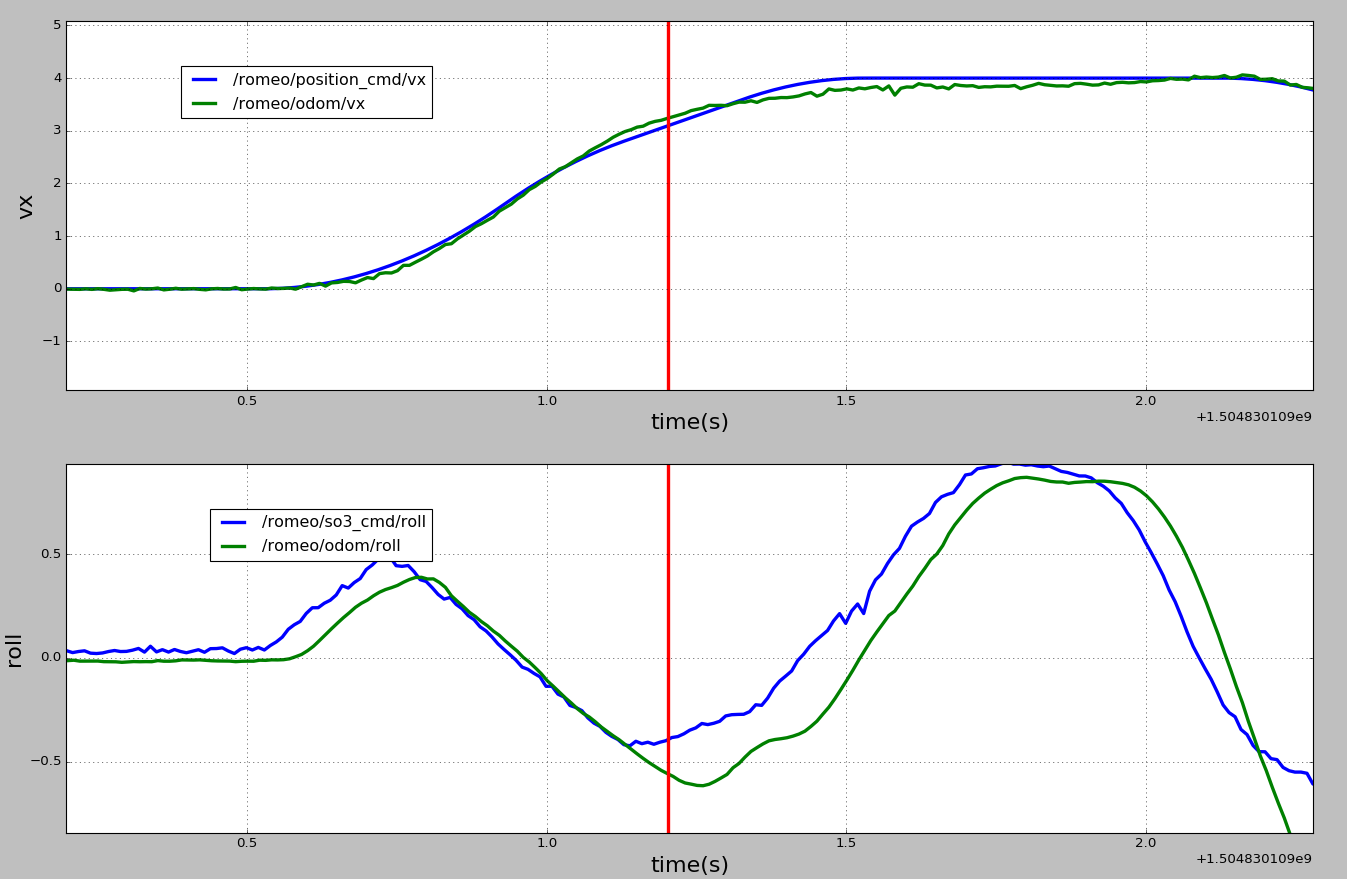
The control errors in velocity and roll are plotted in Fig. 12. The commanded roll includes the feedback attitude errors such that it is not as smooth as the desired roll from the planned trajectory. The robot is able to track velocity properly up to $4m/s$, but clearly there exists lag in the attitude control. This is because the actual robot is not able to achieve specified angular velocity instantly due to the dynamics. A more accurate model for the quadrotor is to use snap as the control input instead of the jerk. The trajectory planned using the snap as the control input is straightforward to solve following the same pipeline as proposed in this paper, which has also been implemented in our open-sourced planner.

References

- [1] S. Liu, M. Watterson, S. Tang, and V. Kumar, “High speed navigation for quadrotors with limited onboard sensing,” in 2016 IEEE International Conference on Robotics and Automation (ICRA). IEEE, 2016.
- [2] C. Richter, A. Bry, and N. Roy, “Polynomial trajectory planning for aggressive quadrotor flight in dense indoor environments,” in Robotics Research. Springer, 2016, pp. 649–666.
- [3] H. Oleynikova, M. Burri, Z. Taylor, J. Nieto, R. Siegwart, and E. Galceran, “Continuous-time trajectory optimization for online uav replanning,” in 2016 IEEE/RSJ International Conference on Intelligent Robots and Systems (IROS), Oct 2016, pp. 5332–5339.
- [4] R. Deits and R. Tedrake, “Efficient mixed-integer planning for uavs in cluttered environments,” in Proceedings of the 2015 IEEE International Conference on Robotics and Automation (ICRA), 2015.
- [5] J. Canny, B. Donald, J. Reif, and P. Xavier, “On the complexity of kinodynamic planning,” in Foundations of Computer Science, 29th Annual Symposium on, 1988, pp. 306–316.
- [6] D. Falanga, E. Mueggler, M. Faessler, and D. Scaramuzza, “Aggressive quadrotor flight through narrow gaps with onboard sensing and computing,” arXiv preprint arXiv:1612.00291, 2016.
- [7] G. Loianno, C. Brunner, G. McGrath, and V. Kumar, “Estimation, control, and planning for aggressive flight with a small quadrotor with a single camera and imu,” IEEE Robotics and Automation Letters, vol. 2, no. 2, pp. 404–411, April 2017.
- [8] T. Hirata and M. Kumon, “Optimal path planning method with attitude constraints for quadrotor helicopters,” in Int. Conf. on Advanced Mechatronic Systems, 2014, pp. 377–381.
- [9] I. Garcia and J. P. How, “Trajectory optimization for satellite reconfiguration maneuvers with position and attitude constraints,” in American Control Conference, 2005, pp. 889–894 vol. 2.
- [10] M. Watterson, T. Smith, and V. Kumar, “Smooth trajectory generation on SE(3) for a free flying space robot,” in IEEE/RSJ Int. Conf. on Intelligent Robots and Systems (IROS), 2016, pp. 5459–5466.
- [11] D. Brescianini and R. D’Andrea, “Design, modeling and control of an omni-directional aerial vehicle,” in 2016 IEEE International Conference on Robotics and Automation (ICRA), May 2016.
- [12] S. Liu, N. Atanasov, K. Mohta, and V. Kumar, “Search-based motion planning for quadrotors using linear quadratic minimum time control,” in IEEE/RSJ Int. Conf. on Intelligent Robots and Systems, 2017.
- [13] D. Mellinger and V. Kumar, “Minimum snap trajectory generation and control for quadrotors,” in Proceedings of the 2011 IEEE International Conference on Robotics and Automation (ICRA), 2011.
- [14] M. J. Van Nieuwstadt and R. M. Murray, “Real time trajectory generation for differentially flat systems,” 1997.
- [15] S. Liu, M. Watterson, K. Mohta, K. Sun, S. Bhattacharya, C. J. Taylor, and V. Kumar, “Planning dynamically feasible trajectories for quadrotors using safe flight corridors in 3-d complex environments,” IEEE Robotics and Automation Letters, vol. 2, no. 3, pp. 1688–1695, July 2017.
- [16] J. Chen, T. Liu, and S. Shen, “Online generation of collision-free trajectories for quadrotor flight in unknown cluttered environments,” in 2016 IEEE International Conference on Robotics and Automation (ICRA). IEEE, 2016, pp. 1476–1483.
- [17] J. Ichnowski and R. Alterovitz, “Fast nearest neighbor search in se (3) for sampling-based motion planning,” in Algorithmic Foundations of Robotics XI. Springer, 2015, pp. 197–214.
- [18] N. Ratliff, M. Zucker, J. A. Bagnell, and S. Srinivasa, “Chomp: Gradient optimization techniques for efficient motion planning,” in IEEE Int. Conf. on Robotics and Automation, 2009, pp. 489–494.
- [19] M. Pivtoraiko, R. A. Knepper, and A. Kelly, “Differentially constrained mobile robot motion planning in state lattices,” Journal of Field Robotics, vol. 26, no. 3, pp. 308–333, 2009.
- [20] B. MacAllister, J. Butzke, A. Kushleyev, H. Pandey, and M. Likhachev, “Path planning for non-circular micro aerial vehicles in constrained environments,” in Robotics and Automation (ICRA), 2013 IEEE International Conference on. IEEE, 2013, pp. 3933–3940.
- [21] M. Mueller, M. Hehn, and R. D’Andrea, “A computationally efficient motion primitive for quadrocopter trajectory generation,” IEEE Trans. on Robotics (T-RO), vol. 31, no. 6, pp. 1294–1310, 2015.
- [22] S. Karaman and E. Frazzoli, “Sampling-based algorithms for optimal motion planning,” The International Journal of Robotics Research (IJRR), 2011.
- [23] E. A. Hansen and R. Zhou, “Anytime heuristic search,” Journal of Artificial Intelligence Research, vol. 28, pp. 267–297, 2007.
- [24] M. Likhachev, G. Gordon, and S. Thrun, “ARA* : Anytime A* with Provable Bounds on Sub-Optimality,” in Advances in Neural Information Processing Systems, 2004, pp. 767–774.
- [25] S. Aine, S. Swaminathan, V. Narayanan, V. Hwang, and M. Likhachev, “Multi-heuristic a,” The International Journal of Robotics Research, vol. 35, no. 1-3, pp. 224–243, 2016.
- [26] C. M. Wilt and W. Ruml, “When does weighted A* fail?” 2012.
- [27] K. Gochev, B. Cohen, J. Butzke, A. Safonova, and M. Likhachev, “Path planning with adaptive dimensionality,” in Fourth annual symposium on combinatorial search, 2011.
- [28] T. Lee, M. Leoky, and N. H. McClamroch, “Geometric tracking control of a quadrotor uav on se (3),” in 49th IEEE conference on decision and control (CDC). IEEE, 2010, pp. 5420–5425.
- [29] M. Hehn and R. D’Andrea, “Quadrocopter trajectory generation and control,” IFAC Proceedings Volumes, vol. 44, no. 1, 2011.
- [30] R. B. Rusu and S. Cousins, “3D is here: Point Cloud Library (PCL),” in IEEE International Conference on Robotics and Automation (ICRA), Shanghai, China, May 9-13 2011.