Strategies to Inject Spoofed Measurement Data
to Mislead Kalman Filter
Abstract
We study the problem of designing false measurement data that is injected to corrupt and mislead the output of a Kalman filter. Unlike existing works that focus on detection and filtering algorithms for the observer, we study the problem from the attacker’s point-of-view. In our model, the attacker can corrupt the measurements by injecting additive spoofing signals. The attacker seeks to create a separation between the estimate of the Kalman filter with and without spoofed signals. We present a number of results on how to inject spoofing signals while minimizing the magnitude of the injected signals. The resulting strategies are evaluated through simulations along with theoretical proofs. We also evaluate the spoofing strategy in the presence of a spoof detector. Building on our main result, we present a strategy that is proven to successfully mislead a Kalman filter while ensuring it is not detected.
Note to Practitioners—This paper is motivated by the need for understanding the limits of how much an adversary can corrupt and mislead the output of a state estimator. We study the problem from the adversary’s point-of-view. We show how an adversary can mislead the output of a Kalman filter by injecting a minimal amount of energy without being detected by a residual-based attack/failure detector. The proposed approach can be applied as an attack strategy to steer the output of a Kalman filter by a desired amount. This is applicable in a variety of scenarios such as target tracking and robot localization. We point out some limitations of the residual-based attack/failure detectors. We expect that this work will lead to a better and more robust state estimator designs in the future.
I Introduction
As autonomous systems proliferate, there are growing concerns about their security and safety [2, 3]. Of particular concern is their vulnerability to signal spoofing attacks [4]. As a result, many researchers are designing algorithms that enable an observer to detect and mitigate signal spoofing attacks (e.g., [5, 6, 7, 8, 9]). We study the problem from the opposite (i.e., the attacker’s) point-of-view. Our goal is to characterize the capabilities of the attacker that is generating the spoofing signals while assuming that the observer is using a Kalman filter for state estimation.
The problem of generating spoofing attacks has been studied specifically for GPS signals. Tippenhauer et al. [4] describe the requirements as well as present a methodology for generating spoofed GPS signals. Larcom and Liu [10] presented a taxonomy of GPS spoofing attacks.
The typical approach to mitigate sensor spoofing attacks is by designing robust state estimators [11]. Fawzi et al. [12] presented the design of a state estimator for a linear dynamical system when some of the sensor measurements are corrupted by an adversarial attacker. We focus on the scenario where the observer uses a Kalman Filter (KF) for estimating the state using measurements that are corrupted by additive spoofing signals by the attackers. We study the problem of generating spoofing signals of minimum energy that can achieve any desired separation between the KF estimate with spoofing and without spoofing. We show that for many practical cases, the spoofing signals can be generated using linear programming in polynomial time.
There has been recent work on designing spoofing attacks for specific systems such as a Linear Quadratic Gaussian controller [13], GPS data [14], wireless sensor networks [15], and electric power grids [16]. In [16], the authors present false data injection attacks, against state estimation in electric power grids. This paper shows that an attacker can exploit the configuration of a power system to launch such attacks to successfully introduce arbitrary errors into certain state variables while bypassing existing techniques for bad measurement detection.
Another work by Su et al. [14] is closely related to ours. The authors show how to spoof the GPS signal without triggering a detector that uses the residual in the Kalman filter. They present a 1-step (greedy) online spoofing strategy that solves a linear relaxation of a Quadratically Constrained Quadratic Program (QCQP) at each timestep. We present a strategy that plans for future timesteps, instead of just the next timestep, while minimizing the spoofing signal energy. Furthermore, we characterize the scenarios under which our strategy finds the optimal solution in polynomial time.
The work that is most closely related to ours is by Mo et al. [13, 15]. Their goal is to design false measurement data to mislead a system with Kalman filter [15] or an LQG control system [13]. Both, our work and the aforementioned work, assume that the system is linear with Gaussian noise and that a discrete Kalman filter is used to estimate the state. Mo et al. [13] define –attacks (see Definitions 2 and 3 in the original paper). Based on their definition, an attack sequence is successful if: (1) the difference in the estimated state of the system under attack and the true state is greater than a given value; and (2) the probability of alarm for the failure detector is always smaller than a given threshold. They proved that a linear control system is perfectly attackable if and only if its transition matrix has an unstable eigenvalue and the corresponding eigenvector satisfies additional conditions (c.f. Theorem 2 in [13]). These conditions may be too strict. We relax the requirements of an attackable system with the goal of being applicable to more classes of systems. Specifically, we remove the second condition in the –attacks and instead we only consider minimizing the total injected signal by . Nevertheless, we also show the conditions under which an attack is successful against an detector.
Bai et al. presented a different notion of a successful attack in two relevant papers [17, 18]. They define a successful attack as --stealthy.11 1 This is not related to the used by Mo et al. [15, 13]. The goal is to maximize the mean squared error between the attacker’s estimated state and the true state subject to . Here, is the Kullback-Leibler divergence (KLD) between the innovation without attack, , and with attack, . Their notion of a successful attack only applies when . Thus, their attack strategy can only be applied when a Kalman filter runs for a long time. Instead, we focus on finite, possibly small, number of time steps and do not require . Furthermore, our notion of a successful attack differs from theirs and does not focus on a specific type of detector.
Various failure detectors have been proposed in the literature. Jones [19] presented one of the first work on failure detection in linear systems. They presented a linear filter that increases the sensitivity of the residual of the filter, which helps to improve the detection of a particular failure. Brumback et al. [20] presented a test for fault detection in Kalman filters. Mo et al.[15] studied the effect of false data injection attacks on state estimation with a failure detectors.
In this paper, we study how to design spoofing signals that are agnostic to the failure detector. The problem is to minimize the magnitude of the injected signals while still ensuring the desired separation in the filter output. We also provide numerical simulations to show our strategy successfully misleads the detector.
Contributions: In this paper, we make the following contributions:
- •
Problem: We formalize the problem of designing false measurement data that is injected to corrupt and mislead the output of a Kalman filter. Intuitively, if the spoofing measurement is large enough, the spoofed estimation will deviate far away from the true state. However, it will be easy to trigger the alarm by potential failure detectors because of the abnormal estimation. Thus, we study how to design and inject the false measurement data to achieve the desired separation with minimal energy of injected data. This is the first work to formalize this problem.
- •
Solution: We present an algorithm to solve this problem and show how to bypass residual-based failure detector:
- –
False data design: We derive the relationship between a spoofed estimation state and the normal state. We show the problem can be solved by Linear Programming optimally and efficiently.
- –
Spoofing with failure detector: We provide strategies and a sufficient condition to design false data for a Kalman filter with a residual-based failure detector (such as a detector) without being detected.
- –
- •
Evaluation: We demonstrate with MATLAB simulations that we can archive any desired separation accurately by injecting false measurement data. We also show that by gradually increasing the separation with a given condition, the attack strategy is able to successfully mislead the detector.
Based on the motion model of the target and the evolution of the KF, three problems for spoofing design are formulated in Section II. Section III shows the approaches to solve these optimization problems. The simulations for verifying spoofing strategies are given in Section IV. Section V provides a numerical example to illustrate how the proposed spoofing strategy can be applied to a system equipped with a failure detector. Finally, Section VI summarizes the conclusion and future work.
II Problem Formulation
Notation: We denote the set of positive real number by , the set of positive integer by . The set of real vectors with dimension is denoted by , and the set of real matrices with rows and columns by . We write as the power of vector norm, as the expectation of a random variable, as the identity matrix with size , and as the normal distribution with mean and variance .
We consider a scenario where an observer estimates the location of a target using a KF in an –dimensional space. The target misleads the observer by adding spoofing signals to the observer’s measurement. We define the target’s model as:
| (1) |
where , is the state of target, is the control input, is the Gaussian process noise with .
The observer estimates the target’s measurement using a linear measurement model:
| (2) |
where and gives the measurement noise with . Note that and are both positive semi-definite matrices.
In order to mislead the observer, the target corrupts the observer’s measurement by adding spoofing signal to mislead the observer’s estimate. We assume the measurement received by the observer is with spoofing signal (Equation (3)) instead of the true measurement without spoofing signal (Equation (2)). The spoofing signal adds additional measurement error:
| (3) |

The observer uses a KF to estimate target’s state with initial distribution . Since it receives the spoofing measurement for updating, we denote distributions generated by the evolution of its KF as when step . We also denote the distributions generated by the evolution of a KF using true measurement as . The goal for the target is to set the separation between the mean estimate and . The target’s spoofing signal is each step within the planning horizon for which some desired separation, , must be achieved (Figure 1). Figure 2 shows the target’s spoofing process where it uses the initial guess of denoted as and desired separation to design spoofing signal . In order to avoid detection, the targets seeks to minimize the magnitude of the spoofing signal.
Note that, although we use the example of tracking a moving target, the state can be more general. For example, it can represent the state of a power system [16], the state of a networked system[15], or the state of a GPS device [10].

We first propose two problems for offline scenarios as follows.
II-A Offline Spoofing Signal Design with Known
If the target knows of the KF, then the target can set equal to .
Problem 1 (Offline with Known ).
Consider a target with motion model (Equation (1)), measurement model (Equation (2)), and spoofing measurement model (Equation (3)). Assume target knows . Find a sequence of spoofing signal inputs, to achieve desired separation between and at step . Such that,
subject to,
| (4) |
where is a weighing parameter and is the optimization horizon.
II-B Offline Spoofing Signal Design with Unknown
Next, we consider the case where the target does not know the initial condition in the KF. Instead, we assume that the initial estimate is not too far away from (in exception).
Problem 2 (Offline with Unknown ).
Consider a target with motion model (Equation (1)), measurement model (Equation (2)), and spoofing measurement model (Equation (3)). Assume the target starts spoofing with , where and . Find a sequence of spoofing signal inputs, to achieve desired separation between and (in expectation) at step . Such that
subject to,
| (5) |
where is a weighing parameters and is the optimization horizon.
III Signal Spoofing Strategies
In this section, we show how to solve Problems 1 and 2 when and . We first present the relationship between the separation and the initial bias .
Theorem 1.
The proof is given in the appendix.
Corollary 1.
The expected value of the separation is,
| (7) |
Proof.
Theorem 1 shows the difference between the two estimated means at step depends on the initial means, and , and the initial covariance matrices and . This is because the Kalman gain depends on the covariance matrix . If target sets and , it has for all since the covariance matrix is updated through the same Kalman prediction and update equation (see appendix). Thus, and then Equation (6) can be simplified as:
As a result, is independent of the measurements when and . Thus, the target can generate spoofing signal inputs by solving Problem 1 offline. Similarly, following Corollary 1, Problem 2 can be saved offline as well.
Problems 1 and 2 are two nonlinear programming problems for arbitrary vector norms . However, when , they can be formulated as linear programming problems. Linear programming can be solved in polynomial time [21]. When , they become QCQP (Quadratically Constrained Quadratic Program). The following shows the LP and QCQP formulations.
Theorem 2.
If and the elements in and are all positive, then Problems 1 and 2 can be solved optimally with linear programming. If and the elements in and are not all positive, then Problems 1 and 2 can be solved optimally with linear programming instances. If and are diagonal matrices, then Problems 1 and 2 can be solved optimally with linear programming.
III-A Linear Programming Formulation for Vector Norm
Here, we show how to formulate Problem 1 using linear programming. A similar procedure can be applied to formulate Problem 2 as linear programming.
The constraint in Problem 1 (Equation 4) follows:
| (9) |
where . is a constant matrix for each and is calculated from the KF iteration with initial covariance and . Since vector norm is the sum of the absolute values of the elements for a given vector, Problem 1 can be directly formulated as a linear programming problem when .
Then we show how to transform this constraint to a standard linear constraint form . To simplify the equation, we use a 2-D case as an example, with . The problem can be extended to dimension follow the same idea. The left side of Equation (9) can be formulated as
| (10) |
where are corresponding coefficients from Equation 6.
Lemma 1.
If the elements in matrices and are positive, then is a linear combination of and , and Problem 1 can be solved as a single LP instance.
Proof.
According to the proof of Theorem 1 appendix, all the coefficients are positive if the elements in matrices and are positive. Therefore, the objective function and the constraints are linear in and . There always exists an optimal solution where all and or where all and . The objective function in both cases will be the same. Without loss of generality, we can assume and , which can be solved using a single LP instance. ∎
The linear programming strategy containing constraints is presented in Algorithm 1. denotes matrix in the linear constraint where and is the collection of nonzero separations .
If Lemma 1 does not hold, it is possible that some elements in can be positive and some are negative. In general, there are four different cases depending on the sign of the first row and the second row for considering each constraint (Equation 10). Then we can obtain four linear optimization problems along four different sub-constraints of each constraint . Thus, in the worst case, the optimal solution can be obtained by solving linear optimization problems. We run Algorithm 1 times by changing the sign of rows in (Line 1) appropriately.
III-B Quadratically Constrained Quadratic Program Formulation for Vector Norm
| (11) |
For simplify the equation, we use a 2-D case as the example, where , , and
Unfortunately, the QCQP formulations for these three problems are NP-hard since the constraint in each problem is concave. If are diagonal matrices, it can be shown that is also a diagonal matrix. We can transform the QCQP formulation to a linear programming problem by using change of variables , and using a procedure similar to .
If is not a diagonal matrix, one solution is to apply the inequality between vector norm and vector norm. The constraint can be changed to vector norm, which is a stricter constraint. A sub-optimal solution can be obtained by using the vector norm.
III-C Receding Horizon: Spoofing with online measurement
Problems 1 and 2 describe the offline versions for spoofing. We also extend the offline problems to an online version. The following formulates an online spoofing scenario.
Consider a target with motion model (Equation (1)), measurement model (Equation (2)), and spoofing measurement model (Equation (3)). Assume the target does not know . It collects a series of measurements from step to current step . Find a sequence of spoofing signal inputs, to achieve desired separation between and (in expectation) within future steps. Such that
| (12) |
where is a weighing parameter, is the current time, and is the predictive time horizon. The target applies as spoofing signal input at each step .
IV Simulations
In this section, we simulate the effectiveness of spoofing strategies for Problems 1, 2 and online case (Section III-C) where a target designs spoofing signals to mislead an observer by achieving the desired separations between and . Our code is available online.22 2 https://github.com/raaslab/signal_spoofing.git
We consider the vector norm and the following models,
Set the weight for all .
For Problem 1, set the initial condition for the KF as,
Since the target knows , it sets and . We first consider a scenario where the target wants to achieve the desired separation at steps, , denoted as , and with the optimization horizon . The target generates a sequence of spoofing signals offline by using a linear programming solver. The spoofing performance is shown in Figure 3-(a) where the true separations are the same as the desired separations. Same successful spoofing achieved when the desired separations are chosen as , as shown in Figure 3-(b).
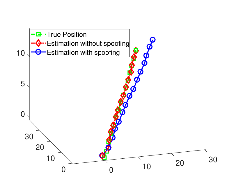
The problem formulation applies in higher dimensional systems as well, not just 2D. Figure 4 shows an example of misleading a KF in a 3D environment.


In Problem 2, the target knows but does not know . The spoofing result is no longer deterministic but holds in expectation . Figure 5-(a) shows spoofing signals for desired separations as with and . Set as , as a random variable () and . In order to see the effectives of the spoofing signals , we conduct 100 trials for each desired separation . Figure 5-(b) shows the is no longer deterministic, but is close to the desired value .
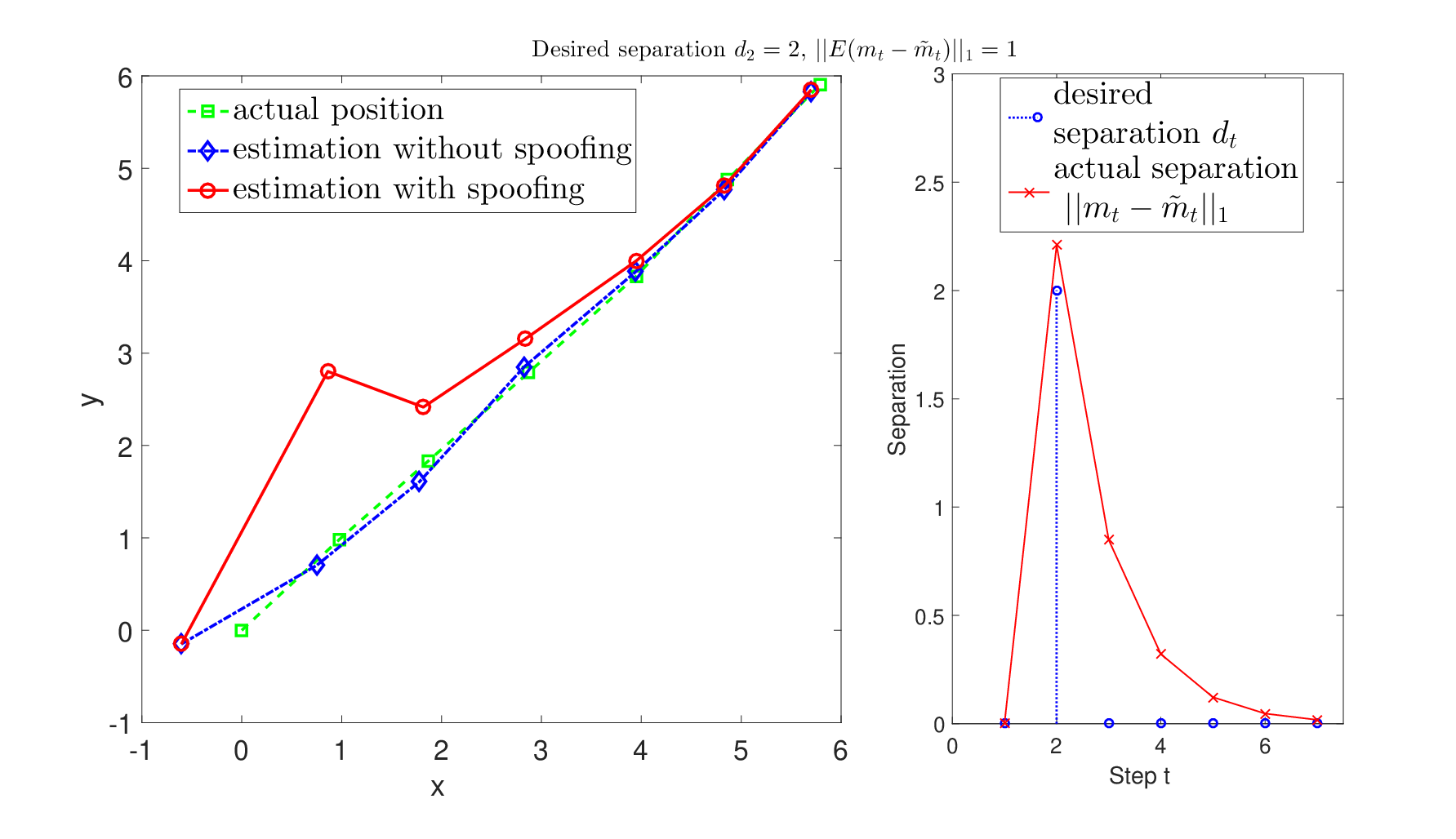

For online case, spoofing signals are continuously generated by using receding horizon optimization with new noisy measurements. We set the receding horizon as . Even though offline strategy performs comparatively as online strategy (Figure 6), online spoofing strategy achieves almost the same separation as the desired, while offline strategy has certain divergence. This is because online strategy can update the measurement at each step.

V Signal spoofing with failure detector
In this section, we evaluate the performance of the false data injection strategy in the presence of a failure detector. We show the conditions (Theorem 3) under which the generated false data can mislead a detector. This result can be also extended to other residual-based detectors.
V-A failure detector
A detector computes the following measure,
| (13) |
where is the innovation or measurement residual of the KF. Here, is the covariance matrix of the residual [23]. The residual is Gaussian since it is the linear combination of two Gaussian random variables. It is known that is distributed with degrees of freedom. If , the detector raises an alarm that the filter is under attack [20].
First, we review the Kalman Filter update equations,
| (14) | ||||
| (15) |
where is the Kalman gain and is given by,
| (16) |
We use the notation, , to indicate the system under attack.
Intuitively, lower the amount of injected attack signal, the less likely it will be detected. This is the motivation behind reducing the energy of the injected system. Nevertheless, when designing an attack sequence over a time horizon, we may have to carefully design the separation sequence so that they are not too large. In the following, we modify notion of a successful attack from [13] and show how to use that to general a successful attack sequence. The differences between two systems are defined as,
| (17) |
Definition 1.
Given , the detector is successfully attacked if there exists an attack sequence such that the following holds:
where is defined above.
Remark 1.
If is bounded, then the difference of its quadratic form is also bounded. Also, as pointed out by [13], by linearity, we can find a , such that .
This definition of successful attack follows the –attack definition by Mo et al. [13]. When the probability of the alarm is bounded and a small enough , the alarm rate will converge to the false alarm rate of the healthy system. Mo et al. [24] presented the relationship between and .
Given the threshold for the detector and , the question is how to set desired separations such that we can avoid being detected. In the following, we give a sufficient condition for designing .
Theorem 3.
If the separations and satisfy , then the proposed algorithm can successfully attack the detector at step .
Proof.
Manipulating Equations (14), (15), (16), and (17), we can prove that,
| (18) |
Taking the norm of Equation (18), we have
| (19) |
Therefore,
| (20) |
We apply the condition of successful attack. If we have,
| (21) |
then,
Note that is a known matrix, and the Kalman gain can be computed from the initial covariance matrix . Hence, we can design the attack sequence for a detector given the threshold . ∎
Theorem 3 shows that if we want to attack a system with detector, the strategy is to make the difference between two consecutive desired separations, and , as small as possible. In general, when we design the attack sequence, we want to increase the separation to mislead the system. Without loss of generality, we can consider the case that all the elements in are non-negative. Given a known separation from previous step , we have the following condition for when we design the desired separation:
| (22) |
Remark 2.
Applying Theorem 3 and Equation (22) and given , we can design a sequence of separations a priori since . For example, if we know the Kalman filter’s initial condition, assuming , we have,
| (23) |
With a known from the proposed LP algorithm, can be designed with the following equation,
| (24) |
Iteratively, we can get the desired separation for all times and guarantee a successful attack ()33 3 Since the inequality is conservative, if the equation converges to , we can add a small term , and let ..
In the following section, we will provide an example that by increasing the separation with given condition. The simulation shows the will not alarm when the separation is designed as Theorem 3.
V-B Simulation with detector
We consider the vector norm and the same model from the simulation section. We use the following parameters:
Given , we can design the separation . The attack result and the detector value are shown in Figure 7.


The differences () between the residual are shown in Figure 8. We ran 1000 trials using this strategy as shown in Figure 7. The detector detected the attack in 112 trials (The false alarm rate is equal to , this rate indicates the detector can not tell whether the alarm is a false alarm or not). This is close to the actual false alarm rate without any attack. In this scenario, the system will not be able to distinguish between false and true alarms. Thus, the attack strategy is able to successfully mislead the detector.
VI Conclusion
We study the problem of injecting spoofing signals to achieve a desired separation in the output of a Kalman filter without and with attack. We study many variants of the problem. Our main approach was to formulate the problems as nonlinear, constrained optimization problems in order to minimize the energy of the spoofing signal. We show that under some technical assumptions, the problems can be solved by linear programming optimally. We present a more computationally expensive approach to solve the problem, without the aforementioned assumptions. We also present a sufficient condition for this strategy to mislead the failure detector.
Our immediate future work is to study the game-theoretic aspects of the problem. In this work, we did not consider any active strategy being employed by the observer to mitigate the attack. In future works, we will consider the case of designing spoofing signals that explicitly take the attack mitigation strategies into account. In all the problems considered in this paper, the desired separations are taken as inputs provided by the user. The simulation results suggest that carefully choosing a specific profile of the desired separation can make it harder to detect by the observer. A possible extension is to automatically generate the optimal profile that not only minimizes the signal energy but also ensures that it is not detected by the observer. Another future work is to extend the strategy to more general non-linear state estimation approaches, such as the extended Kalman filter, unscented Kalman filter, and particle filters.
APPENDIX
VI-A Proof of Theorem 1
Before we prove Theorem 1, we can review the Kalman Filter update equations from equation (17), (14), (15), (16).
According to the Kalman gain update Equation (16), the evolution covariance matrix at step , , only depends on the state model parameters and the initial condition of the covariance matrix . The Kalman gain at step , depends on the covariance matrix . Both and do not depend on the control input series , measurement . Thus, the covariance matrix and the Kalman gain can be predicted from the KF covariance update steps.
| (25) |
From Equation (25), the Kalman gain can be predicted from the initial condition .
We now prove our main result.
Proof.
From the update of KF, we have
| (26) |
and
Recursively,
| (27) |
subtract a term then add the same term,
| (28) |
Define, , and Then,
∎
References
- [1] Z. Zhang, L. Zhou, and P. Tokekar, “Strategies to design signals to spoof kalman filter,” in 2018 Annual American Control Conference (ACC). IEEE, 2018, pp. 5837–5842.
- [2] S. Parkinson, P. Ward, K. Wilson, and J. Miller, “Cyber threats facing autonomous and connected vehicles: Future challenges,” IEEE Transactions on Intelligent Transportation Systems, 2017.
- [3] V. L. Thing and J. Wu, “Autonomous vehicle security: A taxonomy of attacks and defences,” in Internet of Things (iThings) and IEEE Green Computing and Communications (GreenCom) and IEEE Cyber, Physical and Social Computing (CPSCom) and IEEE Smart Data (SmartData), 2016 IEEE International Conference on. IEEE, 2016, pp. 164–170.
- [4] N. O. Tippenhauer, C. Pöpper, K. B. Rasmussen, and S. Capkun, “On the requirements for successful gps spoofing attacks,” in Proceedings of the 18th ACM conference on Computer and communications security. ACM, 2011, pp. 75–86.
- [5] M. Al Faruque, F. Regazzoni, and M. Pajic, “Design methodologies for securing cyber-physical systems,” in Proceedings of the 10th International Conference on Hardware/Software Codesign and System Synthesis. IEEE Press, 2015, pp. 30–36.
- [6] Y. Chen, W. Trappe, and R. P. Martin, “Detecting and localizing wireless spoofing attacks,” in Sensor, Mesh and Ad Hoc Communications and Networks, 2007. SECON’07. 4th Annual IEEE Communications Society Conference on. IEEE, 2007, pp. 193–202.
- [7] S. Gil, S. Kumar, M. Mazumder, D. Katabi, and D. Rus, “Guaranteeing spoof-resilient multi-robot networks,” Autonomous Robots, vol. 41, no. 6, pp. 1383–1400, 2017.
- [8] J. Zhang, R. S. Blum, L. M. Kaplan, and X. Lu, “Functional forms of optimum spoofing attacks for vector parameter estimation in quantized sensor networks,” IEEE Transactions on Signal Processing, vol. 65, no. 3, pp. 705–720, 2017.
- [9] X. Fan, L. Du, and D. Duan, “Synchrophasor data correction under gps spoofing attack: A state estimation based approach,” IEEE Transactions on Smart Grid, 2017.
- [10] J. A. Larcom and H. Liu, “Modeling and characterization of gps spoofing,” in Technologies for Homeland Security (HST), 2013 IEEE International Conference on. IEEE, 2013, pp. 729–734.
- [11] N. Bezzo, J. Weimer, M. Pajic, O. Sokolsky, G. J. Pappas, and I. Lee, “Attack resilient state estimation for autonomous robotic systems,” in Intelligent Robots and Systems (IROS 2014), 2014 IEEE/RSJ International Conference on. IEEE, 2014, pp. 3692–3698.
- [12] H. Fawzi, P. Tabuada, and S. Diggavi, “Secure state-estimation for dynamical systems under active adversaries,” in Communication, Control, and Computing (Allerton), 2011 49th Annual Allerton Conference on. IEEE, 2011, pp. 337–344.
- [13] Y. Mo and B. Sinopoli, “False data injection attacks in control systems,” in First Workshop on Secure Control Systems, CPS Week, Stockholm, Sweden, 2010.
- [14] J. Su, J. He, P. Cheng, and J. Chen, “A stealthy gps spoofing strategy for manipulating the trajectory of an unmanned aerial vehicle,” IFAC-PapersOnLine, vol. 49, no. 22, pp. 291–296, 2016.
- [15] Y. Mo, E. Garone, A. Casavola, and B. Sinopoli, “False data injection attacks against state estimation in wireless sensor networks,” in Decision and Control (CDC), 2010 49th IEEE Conference on. IEEE, 2010, pp. 5967–5972.
- [16] Y. Liu, P. Ning, and M. K. Reiter, “False data injection attacks against state estimation in electric power grids,” ACM Transactions on Information and System Security (TISSEC), vol. 14, no. 1, p. 13, 2011.
- [17] C.-Z. Bai, V. Gupta, and F. Pasqualetti, “On kalman filtering with compromised sensors: Attack stealthiness and performance bounds,” IEEE Transactions on Automatic Control, vol. 62, no. 12, pp. 6641–6648, 2017.
- [18] C.-Z. Bai, F. Pasqualetti, and V. Gupta, “Data-injection attacks in stochastic control systems: Detectability and performance tradeoffs,” Automatica, vol. 82, pp. 251–260, 2017.
- [19] H. L. Jones, “Failure detection in linear systems.” Ph.D. dissertation, Massachusetts Institute of Technology, 1973.
- [20] B. Brumback and M. Srinath, “A chi-square test for fault-detection in kalman filters,” IEEE Transactions on Automatic Control, vol. 32, no. 6, pp. 552–554, 1987.
- [21] N. Karmarkar, “A new polynomial-time algorithm for linear programming,” in Proceedings of the sixteenth annual ACM symposium on Theory of computing. ACM, 1984, pp. 302–311.
- [22] S. Boyd and L. Vandenberghe, Convex optimization. Cambridge university press, 2004.
- [23] S. Thrun, W. Burgard, and D. Fox, Probabilistic robotics. MIT press, 2005.
- [24] Y. Mo and B. Sinopoli, “On the performance degradation of cyber-physical systems under stealthy integrity attacks,” IEEE Transactions on Automatic Control, vol. 61, no. 9, pp. 2618–2624, 2015.