Superstatistical generalised Langevin equation: non-Gaussian viscoelastic anomalous diffusion

However, an additional phenomenon was unveiled in numerous experiments recently. Namely, not only the assumption of normal diffusion is no longer generally valid, numerous experiments have shown a new class of diffusive dynamics in which the fundamental Gaussian property ?? is violated [56, 57, 58, 59]; see also the additional references in [60]. In many of these observations the MSD is still linear, of the form ??, however, the probability density function has the exponential shape (often called Laplace distribution) [61, 56, 62]

How can such observations be explained physically? One of the approaches allowing to explain the emergence of the Laplace distribution is that the measured particle motion does not correspond to samples of the distribution ??, but to a mixture of individual Gaussian processes with different values of the diffusivities $D$. In statistics such an object is called a compound or mixture distribution [63]; in the analysis of diffusion processes this type of model is called superstatistical [64] (which stands for ”superposition of statistics”) or ”doubly stochastic” [65], which is a term for stochastic models generalised by replacing some parameter, for instance, $D$, by a random process. The observations of the Laplace distribution ?? can be justified by assuming that the diffusion coefficient $D$ is a random variable with exponential distribution. Every single trajectory is still Gaussian, but the probability density calculated from the whole ensemble is a compound distribution, in this case exactly the Laplace distribution [56].

There are a few physical interpretations that explain the randomness of $D$. The particles that we observe may not be identical and their different shapes and interactions with the surroundings could and should affect how quickly they diffuse. The environment may also be not homogeneous, which is an expected property of many complex systems, especially biological ones, such as cell membranes. In this situation the diffusion coefficient is local and position dependent $D=D(x)$ [66, 67]. If the particle is moving along trajectory $X(t)$ the effective diffusivity felt is indirectly time-dependent, $D(t)=D(X(t))$. Time dependence can also be direct ($D=D(t,X(t))$) if the environment is changing e.g. because of motion of other particles. Often an approximation is used in which in which $D$ is assumed to evolve independently from $X$. This is a ”diffusing diffusivity” approach proposed by Chubinsky and Slater [68], which is currently being actively developed [69, 70, 60].

According to the superstatistics approach [64] the different diffusivities correspond to the motion of one given particle in a region with a given $D$-value. At sufficiently short time scales the observed particles are relatively localised in such a region, and $D$ can be considered to be constant for each trajectory. The whole ensemble of particles behaves as a system with random $D$ with a distribution of $D$-values mirroring the spacial and temporal dispersion of $D(t,x)$ [71]. Beck proposed that in turbulent media one could consider the Langevin equation ?? to be valid, however, the effective temperature is random such that $(k_{B}T)^{-1}$ is distributed according to $\chi^{2}$ statistics [72, 64, 73].

We note here that viscoelastic anomalous diffusion with Laplace shape of the probability density function was observed for the motion of messenger RNA molecules in the cytoplasm of bacteria and yeast cells [74, 75], while stretched Gaussian shapes were unveiled in the motion of lipids in protein-crowded lipid biliayer systems [76].

In what follows we study a natural extension of this idea: what if not the temperature, but the properties of the stochastic force in equations ?? and ?? is random? Such an assumption may be justified in the same way as the randomness of $D$. Namely, this situation can be realised in an ensemble of particles with varying systems parameters, or in non-homogenous media. This approach resembles to some degree models such as the GLE with kernels, that are a mixture of more elementary functions [77, 43]. Similar ideas appear in financial modelling with ”gamma-mixed Ornstein-Uhlenbeck process” [78]. However in these models the observed trajectories are not examples of compound distributions but result from deterministic dynamics, which can be interpreted as an average over random local dynamical laws. In our approach the studied processes are truly superstatistical.

The paper is structured as follows. In section 2 we introduce the GLE with random parameters and discuss its elementary properties. Section 3 then considers the concrete case of a compound Ornstein-Uhlenbeck process within the superstatistical approach. In section 4 more complex types of memory are proposed and studied, including oscillatory regimes. Our findings are discussed in section 5. In the appendix some more technical details are presented.

The classical Langevin equation can be considered as an approximation of the GLE in which the covariance function $r_{\xi}$ decays very rapidly in the relevant time scale. The solution of the Langevin equation exhibits many properties typical to the GLE in general. We fix the mass of the particle and the bath temperature, so equation ?? is governed solely by the parameter $\lambda$. The superstatistical solution is thus $V_{\Lambda}$, where $\Lambda>0$ is a random variable, which can be interpreted as a local viscosity value. The Langevin equation can be solved using the integrating factor $\exp(\Lambda t)$, which yields the stationary solution

The solution $V_{\lambda}$ for fixed $\lambda$ is often called Ornstein-Uhlenbeck process, so $V_{\Lambda}$ may be called a compound Ornstein-Uhlenbeck process. It can also be represented in Fourier space. Calculating the Fourier transform of equation ?? demonstrates that

where we note that the Fourier transform of Gaussian white noise $\widehat{\xi}$ is another Gaussian white noise. Another useful representation is the recursive formula, which is fulfilled by process in discretised time moments. If we solve the Langevin equation ?? using the integrating factor $\exp(\Lambda t)$ but integrate from time $k\Delta t$ to $(k+1)\Delta t$ we obtain

where the noise $Z_{k}$ has the same distribution as a Gaussian discrete white noise $\xi_{k}$ multiplied by a random constant. The series $Z_{k}$ is, conditionally on $\Lambda$, independent from past values $V_{\Lambda}(j\Delta t)$, with $j<k$. Such a process is called a random-coefficient autoregressive process of order 1, in short AR(1) [93, 94] with autoregressive coefficient $\exp(-\Delta t\Lambda)$. When there are only few distinct populations and $\Lambda$ has only few possible values, they can even be recognised on the phase plot of $y=V_{\Lambda}((k+1)\Delta t)$ versus $x=V_{\Lambda}(k\Delta t)$, see Figure 1. There, the two distinct populations with different autoregressive coefficients can be distinguished. Both have Gaussian distribution, but each one has a distinct elliptical shape. The total distribution, as a mixture of two ellipsoids, is not Gaussian, nor even elliptical. The projection of the joint distribution on $x$ or $y$ axis are the PDF of $V_{\Lambda}(t)$ and are Gaussian, thus, one needs at least a two-dimensional phase plot to reveal the non-Gaussianity of $V_{\Lambda}$. For a larger number of populations the phase plot would be much less clear, but the huge advantage of this method is that it works even for trajectories of very short length.

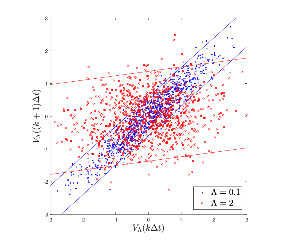
The situation becomes more complex and interesting when $\Lambda$ assumes a continuous distribution. The covariance function of the Ornstein-Uhlenbeck process is

Here some care needs to be taken, as the factor $1/2$ differs from the covariance of the solution of the GLE for which generally $r_{V}(0)=1$ (this is due to the fact that it corresponds to a degenerate Dirac delta kernel). If $\Lambda$ has the PDF $p_{\Lambda}$, the covariance function of $V_{\Lambda}$ is

so it is the Laplace transform of $p_{\Lambda}$: in probabilistic language this quantity would be called a moment generating function of the variable $-\Lambda$. For instance, if $\Lambda$ is a stable subordinator with index $0<\alpha<1$ [95] the covariance function is the stretched exponent

which is a common relaxation model [96, 97, 98, 100], sometimes referred to as Kohlrausch-Williams-Watts relaxation [101, 102].

If $\Lambda$ can be decomposed into a sum of two independent random variables $\Lambda=\Lambda_{1}+\Lambda_{2}$, the corresponding covariance function is a product,

Therefore, in this model various kinds of truncations of the kernel correspond to a decomposition of $\Lambda$, for instance, if $\Lambda=\lambda+\Lambda^{\prime}$ with deterministic $\lambda>0$, the covariance function $r_{V_{\Lambda}}$ will be truncated by $\exp(-\lambda t)$.

Some general observations about the behaviour of $r_{V_{\Lambda}}$ can be made. When $\Lambda$ has a distribution supported on an interval, such as $\lambda_{1}<\Lambda<\lambda_{2}$, and its PDF has no singularity, it is necessarily bounded, that is, $m\leq p_{\Lambda}(\lambda)\leq M$. In this case,

The integrals on the left and right have asymptotics of the form

Here we introduce the notation of an asymptotic inequality, which will be useful later on. We write $f\lesssim g$ if $f\sim h\leq g$ for some function $h$.³³ 3 This is similar to the Landau-$\mathcal{O}$ notation, but when we write $\lesssim$ we also include the value of the constant factor which would be omitted writing $r_{V_{\Lambda}}=\mathcal{O}(t^{-1}\rme^{-\lambda_{1}t})$. Using this notion we can write the above results as

This equation proves that $c_{1}t^{-1}\rme^{-\lambda_{1}t}\lesssim r_{V_{\Lambda}}(t)\lesssim c_{2}t^{-1}\rme^{-\lambda_{1}t}$ for some constants $0<c_{1}<c_{2}$. Further on we will denote this property by $r_{V_{\Lambda}}\asymp t^{-1}\rme^{-\lambda_{1}t}$.⁴⁴ 4 The same situation is sometimes denoted in terms of the ”large theta” notation, that is $r_{V_{\Lambda}}=\Theta(t^{-1}\rme^{-\lambda_{1}t})$. When $\Lambda$ is distributed uniformly, $m=M=(\lambda_{2}-\lambda_{1})^{-1}$, and the asymptotic $\asymp$ becomes stronger, that is, $r_{V_{\Lambda}}(t)\sim(2(\lambda_{2}-\lambda_{1})t)^{-1}\rme^{-\lambda_{1}t}$. This distribution of $\Lambda$ is important from a practical standpoint, because it is a maximal entropy distribution supported on the interval $[\lambda_{1},\lambda_{2}]$, so it can be interpreted as the choice taken using the weakest possible assumptions.

Heavier tails of $r_{V_{\Lambda}}$ may be observed only when the distribution of $\Lambda$ is concentrated around $0^{+}$.The most significant case of such a distribution is a power law of the form $p_{\Lambda}(\lambda)\sim\lambda^{\alpha-1}$, with $\lambda\to 0^{+}$ and $\alpha>0$. For any distribution of this type Tauberian theorems guarantee that the tail of the covariance has a power law tail [103, 104]

For $\alpha<1$ the process $V_{\Lambda}$ exhibits a long memory. This observation can be refined as follows. In Proposition 2 i) we present a generalised Tauberian theorem, which states that if the PDF of $\Lambda$ contains slowly-varying factor $L$, then the tail of the covariance contains the factor $L(t^{-1})$. One example of such a slowly-varying factor is $|\ln(\lambda)|^{\beta},\beta>0$, so heavy tails of the covariance of the power law form $t^{-\alpha}\ln(t)^{\beta}$ can also be present for compound Ornstein-Uhlenbeck process if the distribution of $\Lambda$ exhibits a logarithmic behaviour at $0^{+}$. This observation proves that this equation can also describe ultra-slow diffusion and can be considered as an alternative to more complex models based on distributed order fractional derivatives [105, 77].

In Section 2 we noted that the superstatistical solutions of the Langevin equations are not Gaussian, however, they can be easily mistaken to be Gaussian. The marginal distributions of $V_{\Lambda}$ are Gaussian at any time $t$, only the joint distributions are not. This means that the multidimensional PDF of the variables $V_{\Lambda}(t_{1}),V_{\Lambda}(t_{2}),\ldots,V_{\Lambda}(t_{n})$ does not have Gaussian shape. This fact is easy to observe studying the characteristic function of the two point distribution, which is a Fourier transform of the two-point PDF. Let us fix $V_{\Lambda}(\tau)$, $V_{\Lambda}(\tau+t)$ and define the two-point characteristic function as

For any deterministic $\lambda$ this function is determined by the covariance matrix $\Sigma_{t}$ of the pair $V_{\lambda}(\tau),V_{\lambda}(\tau+t)$,

so in the superstatistical case the characteristic function reads

As we argued, the marginal factors $\exp(-\theta_{1}^{2}/4),\exp(-\theta_{2}^{2}/4)$ are indeed Gaussian, but the cross factor describing the interdependence is not. The function $\phi_{\Lambda}$ would describe a Gaussian distribution if and only if the factor $\mathbb{E}\left[\exp(\theta_{1}\theta_{2}\rme^{-\Lambda t}/2)\right]$ had the form $\exp(a\theta_{1}\theta_{2})$. But we see that it is in fact a moment generating function of the variable $\exp(-\Lambda t)$ at point $\theta_{1}\theta_{2}/2$, which is an exponential if and only if $\Lambda$ equals one fixed value with probability unity. The compound Ornstein-Uhlenbeck is never Gaussian for non-deterministic $\Lambda$.

This property is also evident if we calculate the conditional MSD of $X_{\Lambda}$,

At short times $t$ this approximately is $t^{2}/4$, so the distribution is nearly Gaussian and the motion is ballistic. However at long $t$ the dominating term is $(2\Lambda)^{-1}t$, so we see that if $\mathbb{E}[\Lambda^{-1}]<\infty$, the integrated compound Ornstein-Uhlenbeck process describes normal diffusion with random diffusion coefficient $D=(4\Lambda)^{-1}$. Such a situation occurs when the distribution $\Lambda$ is not highly concentrated around $0^{+}$. When $\Lambda$ has a power-law singularity as in ??, that is $\lambda^{\alpha-1}$ at $0^{+}$, $0<\alpha<1$, this condition is not fulfilled: $\mathbb{E}[\Lambda^{-1}]=\infty$. But in this situation the assumptions required for the Tauberian theorem hold and we can apply it twice: first for relation ??, to show that $\widetilde{r_{V_{\Lambda}}}(s)\sim 2^{-1}\Gamma(\alpha)\Gamma(1-\alpha)s^{\alpha-1},s\to 0^{+}$ and the second time for relation ??, to prove that

In this regime the system is superdiffusive. The transition from superdiffusion ($0<\alpha<1$) to normal diffusion ($1\leq\alpha$) is unusual among diffusion models. Fractional Brownian motion and fractional Langevin equation [46, 106, 41] undergo transitions from super- to subdiffusion at a critical point of the control parameter. This is so as in these models in this the change of the diffusion type is caused by the change of the memory type from persistent to antipersistent. But the Ornstein-Uhlenbeck process models only persistent dependence, so the mixture of such motions also inherits this property. For $1\leq\alpha$ (and any other case when $\mathbb{E}[\Lambda^{-1}]<\infty$) this dependence is weak enough for the process to be normally diffusive, for smaller values of $\alpha$ it induces superdiffusion.

In the introduction we already mentioned that it is commonly observed that the distribution of the position process is double exponential, see equation ?? and references below. This exact distribution is observed when $D$ has an exponential distribution $\mathcal{E}(\beta)$ with PDF

For the corresponding compound Ornstein-Uhlenbeck process the distribution of $\Lambda$ is given by $\Lambda=(4D)^{-1}$ and for such a choice the process models normal diffusion with a Laplace PDF. Moreover the covariance function of the velocity process is

where we used one of the integral representations of the modified Bessel function of the second kind $K_{1}$ (see [107], formula 10.32.10). This function has the asymptotic $K_{1}(z)\sim\sqrt{\pi/2}\exp(-z)z^{-1/2}$, $z\to\infty$ ([107], formula 10.40.2), so the covariance function behaves like

This behaviour is shown in Figure 2, where we present the covariance function corresponding to the Laplace distributed $X_{\Lambda}(t)$ with random diffusion coefficient $D\overset{d}{=}\mathcal{E}(2)$. We do not present the Bessel function ??, as it appears to be indistinguishable from the result of the Monte Carlo simulation. Figure 2 also shows how to distinguish this behaviour from an exponential decay on a semi-logarithmic scale: the covariance function and its asymptotic are concave, which is mostly visible for short times $t$.

Analysing the shape of the covariance function can serve as a method to distinguish between a superstatistic introduced by a local effective temperature and the distribution of mass from superstatistics caused by the randomness of the viscosity $\Lambda$. In the former case the resulting decay is exponential (as in the non-superstatistical Langevin equation) or even zero for a free Brownian particle, in the latter case it is given by relation ??.

In order to better understand the superstatistical Langevin equation we will consider a simple model with one particular choice for the distribution $\Lambda$. After going through this explicit example we will come back to the general case at the end of this section.

A generic choice for the $\Lambda$ distribution is the Gamma distribution $\mathcal{G}(\alpha,\beta)$ with the PDF

This corresponds to a power law at $0^{+}$ which is truncated by an exponential. As the conditional covariance function is an exponential, too, many integrals which in general would be hard to calculate, in this present case turn out to be surprisingly simple.

The Gamma distribution is also a convenient choice because many of its special cases are well established in physics. The Erlang distribution is the special case of expression ?? when $\alpha$ is a natural number. An Erlang variable with $\alpha=k$ and $\beta$ can be represented as the sum of $k$ independent exponential variables $\mathcal{E}(\beta)$, in particular, for $k=1$ it is the exponential distribution itself. The Chi-square distribution $\chi^{2}(k)$ is also a special case of expression ?? where $\alpha=k/2,\beta=1/2$. The Maxwell-Boltzmann distribution corresponds to the square root of $\chi^{2}(3)$, and the Rayleigh distribution to the square root of $\chi^{2}(2)$.

We already know from relation ?? that $r_{V_{\Lambda}}$ has a power tail $\sim 2^{-1}\beta^{\alpha}t^{-\alpha}$, more specifically, direct integration yields

This is solely a function of the ratio $t/\beta$ which suggests that the parameter $\beta$ changes the time scale of the process. Indeed, for any $\lambda$ the process $V_{\lambda}(bt)$ is equivalent to $V_{b\lambda}(t)$, because the Gaussian process is determined by its covariance function, which in both cases is the same. Therefore, also the compound process $V_{\Lambda}(bt)$ is equivalent to $V_{b\Lambda}(t)$ and $b\Lambda$ has the distribution $\mathcal{G}(\alpha,\beta/b)$.

The function ?? would be observed if we calculated the ensemble average of $V_{\Lambda}(\tau)V_{\Lambda}(\tau+t)$ for some $\tau$. If instead the covariance function would be estimated as a time average over individual trajectories, the Birkhoff theorem determines that the result would be a random variable, equal to the conditional covariance

It is straightforward to calculate the PDF of this distribution,

The mean value of this quantity is given by result ??. This PDF is zero in the point $x=1/2$ if $\alpha>1$ but has a logarithmic singularity at $x=(1/2)^{-}$ if $\alpha<1$ (that is, in the long-memory case). It is zero in $x=0$ for $t<\beta$ as in expression ?? any power law dominates any power of the logarithm. For $t>\beta$ there is a singularity at $x=0^{+}$ which approaches the asymptotics $x^{-1}|\ln x|^{\alpha-1}$ as $t\to\infty$. This behaviour can be observed in Figure 3, illustrating how the probability mass moves from $(1/2)^{-}$ to $0^{+}$ as time increases.

As we already know, the compound Ornstein-Uhlenbeck process is non-Gaussian. Let us follow up on this property in more detail. To study the characteristic function we need to calculate the average in equation ??, which is actually the moment generating function for the random variable $\exp(-\Lambda t)$. Some approximations can be made. First, let us assume that $\Lambda t$ is small in the sense that the probability that this variable is larger than some small $\epsilon>0$ is negligible. In this regime we can approximate $\exp(-\Lambda t)\approx 1-\Lambda t$ and find

The first factor describes a distribution of $V_{\Lambda}(\tau)=V_{\Lambda}(\tau+t)$. So in our approximation we assume that the values in the process between short time delays are nearly identical and the multiplicative correction $(1-t\theta_{1}\theta_{2}/(2\beta))^{-\alpha}$ is non-Gaussian.

The second type of approximation can be made for long times $t$ when $\exp(-\Lambda t)\approx 0$. In this case

Now we treat the values $V_{\Lambda}(\tau)$ and $V_{\Lambda}(\tau+t)$ as nearly independent, the small correction is once again non-Gaussian. Apart from the approximations, the exact formula for $\phi_{\Lambda}$ can be provided using the series

which is absolutely convergent.

Note that for the specific choice $\theta_{1}=\theta$, $\theta_{2}=-\theta$ the function $\phi_{\Lambda}$ is a Fourier transform of the probability density of the increment $\Delta V_{\Lambda}(\tau,t)\mathrel{\mathop{:}}=V_{\Lambda}(\tau)-V_{\Lambda}(\tau+t)$, which therefore equals

Clearly, any increment of $V_{\Lambda}$ is non-Gaussian. This is demonstrated in Figure 4, where we show $\sqrt{-\ln(\widehat{p}_{\Delta V_{\Lambda}(\tau,1)}(\theta))}$ on the y-axis. In this choice of scale Gaussian distributions are represented by straight lines. The concave shape of the empirical estimator calculated using Monte Carlo simulation shows that the process $V_{\Lambda}$ is indeed non-Gaussian. In the same plot we present the two types of approximations of $\widehat{p}_{\Delta V_{\Lambda}(\tau,1)}$: for $t\to 0^{+}$ we have equation ??, which reflects well the tails $\theta\to\pm\infty$, and for $t\to\infty$ we see that with several terms of the series ?? a good fit for $\theta\approx 0$ is obtained.

It may appear counter-intuitive that the values $V_{\Lambda}(t)$, which are all exactly Gaussian, are sums of non-Gaussian variables. If the increments were independent that would be impossible, here their non-ergodic dependence structure allows for this unusual property to emerge. However, the they are still conditionally Gaussian with variance

References

- [1] Einstein A 1905 Ann. der Physik
- [2] von Smoluchowski M 1906 Ann. der Physik 326 756–780
- [3] Lemons D and Gythiel A 1997 Am. J. Phys. 65 1079–1081
- [4] Wiener N 1921 Proc. Natl. Acad. Sci. U.S.A. 7 294–298
- [5] Lucretius 2008 De rerum natura. (On the Nature of the Universe) (Oxford University Press)
- [6] Hughes B 1995 Random walks and random environments vol 1 (Oxford University Press)
- [7] Coffey W and Kalmykov Y 2012 The Langevin equation (World Scientific)
- [8] Metzler R and Klafter J 2000 Phys. Rep. 339 1–77
- [9] Höfling F and Franosch T 2013 Rep. Prog. Phys. 76 046602
- [10] Nørregaard K, Metzler R, Ritter C, Berg-Sørensen K and Oddershede L 2017 Chem. Rev. 117 4342–4375
- [11] Weiss M, Hashimoto H and Nilsson T 2003 Biophys. J. 84(6) 4043–4052
- [12] Jeon J H, Tejedor V, Burov S, Barkai E, Selhuber-Unkel C, Berg-Sørensen K, Oddershede L and Metzler R 2011 Phys. Rev. Lett. 106(4) 048103
- [13] Yang H, Luo G, Karnchanaphanurach P, Louie T M, Rech I, Cova S, Xun L and Xie X S 2003 Science 302 262–266
- [14] Kou S C and Xie X S 2004 Phys. Rev. Lett. 93(18) 180603
- [15] Golding I and Cox E 2006 Phys. Rev. Lett. 96(9) 098102
- [16] Tabei S M A, Burov S, Kim H Y, Kuznetsov A, Huynh T, Jureller J, Philipson L, Dinner A and Scherer N 2013 Proc. Natl. Acad. Sci. USA 110 4911–4916
- [17] di Rienzo C, Piazza V Gratton E, Beltram F and Cardarelli F 2014 Nat. Commun. 5(5891)
- [18] Szymanski J and Weiss M 2009 Phys. Rev. Lett. 103(3) 038102
- [19] Wong I Y, Gardel M L, Reichman D R, Weeks E R, Valentine M T, Bausch A R and Weitz D A 2004 Phys. Rev. Lett. 92(17) 178101
- [20] Banks D and Fradin C 2005 Biophys. J. 89(5) 2960–2971
- [21] Jeon J-H, Leijnse N, Oddershede L and Metzler R 2013 New J. Phys. 15 045011
- [22] Jeon J-H, Monne H M S, Javanainen M and Metzler R 2012 Phys. Rev. Lett. 109(18) 188103
- [23] Bakalis E, Höfinger S, Venturini A and Zerbetto F 2015 J. Chem. Phys. 142 215102
- [24] Akimoto T, Yamamoto E, Yasuoka K, Hirano Y and Yasui M 2011 Phys. Rev. Lett. 107(17) 178103
- [25] Kneller G, Baczynski K and Pasenkiewicz-Gierula M 2011 J Chem Phys. 135 141105
- [26] Javanainen M, Martinez-Seara H, Metzler R and Vattulainen I 2017 J. Phys. Chem. Lett 8 4308–4313
- [27] Caspi A, Granek R and Elbaum M 2000 Phys. Rev. Lett. 85(26) 5655–5658
- [28] Reverey J, Bao H, Jeon J-H, Leippe M, Metzler R and Selhuber-Unkel C 2015 Sci. Rep. 5
- [29] Despósito M, Pallavicini C, Levi V and Bruno L 2011 Physica A 390 1026 – 1032
- [30] Goychuk I, Kharchenko V and Metzler R 2014 Phys. Chem. Chem. Phys. 16(31) 16524–16535
- [31] Richardson L 1926 Proc. Roy. Soc. A 110 709–737
- [32] Budaev V, Takamura S, Ohno N and Masuzaki S 2006 Nucl. Fusion 46 S181
- [33] Liu B and Goree J 2008 Phys. Rev. Lett. 100 055003
- [34] Perri1 S, Zimbardo1 G, Effenberger F and Fichtner H 2015 A& A 578
- [35] Rogers L and Williams D 1994 Diffusions, Markov Processes, and Martingales 2nd ed (Wiley)
- [36] Metzler R, Jeon J-H, Cherstvy A G and Barkai E 2014 Phys. Chem. Chem. Phys. 16 24128–24164
- [37] Kubo R 1966 Rep. Prog. Phys. 29 255–284
- [38] Hänggi P, Talkner P and Borkovec M 1990 Rev. Mod. Phys. 62(2) 251–341
- [39] Zwanzig R 2001 Nonequlibrium Statistical Mechanics (Oxford University Press)
- [40] Weiss U 2008 Quantum Dissipative Systems (Word Scientific)
- [41] Kou S C 2008 Ann. Appl. Stat. 2 501–535
- [42] Sandev T, Metzler R and Tomovski Ž 2014 J. Math. Phys. 55 023301
- [43] Tateishi A A, Lenzi E K, da Silva L R, Ribeiro H V, Picoli S and Mendes R S 2012 Phys. Rev. E 85(1) 011147
- [44] Goychuk I 2009 Phys. Rev. E 80(4) 046125
- [45] Wang K and Tokuyama M 1999 Physica A 265 341–351
- [46] Lutz E 2001 Phys. Rev. E 64(5) 051106
- [47] Deng W and Barkai E 2009 Phys. Rev. E 79(1) 011112
- [48] Ford G, Kac M and Mazur P 1965 J. Math. Phys. 6 504–515
- [49] Zwanzig R 1973 J. Stat. Phys 9 215–220
- [50] Rey-Bellet L 2006 Open classical systems Quantum Dissipative Systems II (Springer-Verlag) pp 41–78
- [51] Pavliotis G 2014 Stochastic Processes and Applications (Springer-Verlag)
- [52] Rouse Jr P 1953 J. Chem. Phys. 21 1272–1280
- [53] Panja D 2010 J. Stat. Mech. 2010 L02001
- [54] Lizana L, Ambjörnsson T, Taloni A, Barkai E and Lomholt M 2010 Phys. Rev. E 81(5) 051118
- [55] Kneller G 2011 J. Chem. Phys. 134 224106
- [56] Wang B, Kuo J, Bae S and Granick S 2012 Nat. Mat. 11
- [57] Metzler R, Jeon J-H and Cherstvy A 2016 Biochim. Biophys. Acta-Biomembranes 1858 2451 – 2467
- [58] Jeon J-H, Javanainen M, Martinez-Seara H, Metzler R and Vattulainen I 2016 Phys. Rev. X 6(2) 021006
- [59] Metzler R 2017 Biophys. J. 112(3) 413–415
- [60] Chechkin A, Seno F, Metzler R and Sokolov I 2017 Phys. Rev. X 7(2) 021002
- [61] Wang B, Anthony S, Bae S and Granick S 2009 Proc. Natl. Acad. Sci. U.S.A. 106 15160–15164
- [62] Bhattacharya S, Sharma D, Saurabh S, De S, Sain A, Nandi A and Chowdhury A 2013 J. Phys. Chem. B 117 7771–7782
- [63] Lindsay B G 1995 NSF-CBMS Reg. Conf. Ser, in Prob. Stat. 5 i–163
- [64] Beck C and Cohen E 2003 Physica A 322 267 – 275
- [65] Tjøstheim D 1986 J. Time Ser. Anal. 7 51–72
- [66] Olivares-Rivas W, Colmenares P and López F 2013 J. Chem. Phys. 139 074103
- [67] Hummer G 2005 New J. Phys. 7 34
- [68] Chubynsky M and Slater G 2014 Phys. Rev. Lett. 113(9) 098302
- [69] Cherstvy A and Metzler R 2016 Phys. Chem. Chem. Phys. 18(34) 23840–23852
- [70] Jain R and Sebastian K 2016 J. Phys. Chem. B 120 3988–3992
- [71] Manzo C, Torreno-Pina J, Massignan P, Lapeyre G, Lewenstein M and Garcia P M F 2015 Phys. Rev. X 5(1) 011021
- [72] Beck C 2001 Phys. Rev. Lett. 87(18) 180601
- [73] Beck C 2006 Prog. Theor. Phys. Suppl. 162 29–36
- [74] Lampo T, Stylianido S, Backlund M, Wiggins P and Spakowitz A 2017 Biophys. J. 112(3) 532–542
- [75] Metzler R 2017 Biophys. J. 112(3) 413–415
- [76] Jeon J-H, Javanainen M, Martinez-Seara H, Metzler R and Vattulainen I 2016 Phys. Rev. X 6(2) 021006
- [77] Sandev T and Tomovski Ž 2014 Phys. Lett. A 378(1-2) 1–9
- [78] Igloi E and Terdik G 1999 Electron. J. Probab. 4 33 pp.
- [79] Touchette H and Beck C 2005 Phys. Rev. E 71(1) 016131
- [80] Van der Straeten E and Beck C 2008 Phys. Rev. E 78(5) 051101
- [81] Perrin J 1908 Compt. Rend. (Paris) 146 967
- [82] Perrin J 1909 Ann. Chim. Phys. 18 1–114
- [83] Norlund I 1914 Z. Phys. Chem. 87 40
- [84] Barkai E, Garini Y and Metzler R 2012 Phys. Today 65(8) 29
- [85] Maruyama G 1970 Theory Probab. Appl. 15 1–22
- [86] Dym H and McKean H P 1976 Gaussian Processes, Function Theory and the Inverse Spectral Problem (Academic Press)
- [87] Ślęzak J 2017 Ann. Phys 383 285 – 311
- [88] Jeon J-H and Metzler R 2012 Phys. Rev. E 85(2) 021147
- [89] Kursawe J, Schulz J and Metzler R 2013 Phys. Rev. E 88(6) 062124
- [90] Doob J L 1990 Stochastic Processes (Wiley-Interscience)
- [91] He Y, Burov S, Metzler R and Barkai E 2008 Phys. Rev. Lett. 101(5) 058101
- [92] Cherstvy A, Chechkin A and Metzler R 2013 New J. Phys. 15 083039
- [93] Brockwell P and Davis R 2006 Time Series: Theory and Methods (Springer-Verlag)
- [94] Box J and Jenkins G 1994 Time Series Analysis: Forecasting and Control (Prentice-Hall)
- [95] Samorodnitsky G and Taqqu M 1994 Stable Non-Gaussian Random Processes (Chapman & Hall)
- [96] Kakalios J, Street R and Jackson W 1987 Phys. Rev. Lett. 59(9) 1037–1040
- [97] Piazza R, Bellini T, Degiorgio V, Goldstein R, Leibler S and Lipowsky R 1988 Phys. Rev. B 38(10) 7223–7226
- [98] Köpf M, Corinth C, Haferkamp O and Nonnenmacher T 1996 Biophys. J. 70 2950 – 2958
- [99] Williams G and Watts D 1970 Trans. Faraday Soc. 66(0) 80–85
- [100] Weron K and Kotulski M 1996 Physica A 232 180–188
- [101] Kohlrausch R 1847 Pogg. Ann. Phys. (Leipzig) 12(3) 393
- [102] Williams G and DC W 1970 Trans. Faraday Soc. 66 80
- [103] Feller W 1968 An Introduction to Probability Theory and Its Applications 3rd ed (Wiley)
- [104] Postnikov A 1980 Tauberian Theory and Its Applications (American Mathematical Society)
- [105] Eab C and Lim S 2011 Phys. Rev. E 83
- [106] Burov S and Barkai E 2008 Phys. Rev. E 78(3) 031112
- [107] NIST Digital Library of Mathematical Functions Release 1.0.15 of 2017-06-01 URL http://dlmf.nist.gov/
- [108] Haubold H, Mathai A and Saxena R 2011 J. Appl. Math. 2011
- [109] Gorenflo R, Kilbas A, Mainardi F and Rogosin S 2014 Mittag-Leffler Functions, Related Topics and Applications (Springer-Verlag)