Gravitational self-interactions of a degenerate
quantum scalar field

Sankha S. Chakrabarty, Seishi Enomoto, Yaqi Han, Pierre Sikivie and Elisa M. Todarello Affiliation: Department of Physics, University of Florida, Gainesville, FL 32611, USA

January 16, 2018

Abstract

We develop a formalism to help calculate in quantum field theory the departures from the description of a system by classical field equations. We apply the formalism to a homogeneous condensate with attractive contact interactions and to a homogeneous self-gravitating condensate in critical expansion. In their classical descriptions, such condensates persist forever. We show that in their quantum description, parametric resonance causes quanta to jump in pairs out of the condensate into all modes with wavevector less than some critical value. We calculate in each case the time scale over which the homogeneous condensate is depleted, and after which a classical description is invalid. We argue that the duration of classicality of inhomogeneous condensates is shorter than that of homogeneous condensates.

pacs

95.35.+d

I Introduction

The identity of dark matter remains one of the foremost questions in science today [1]. One of the leading candidates is the QCD axion, which has the double virtue of solving the strong CP problem of the standard model of elementary particles [2, 3] and of being naturally produced with very low velocity dispersion in the early universe [4], so that it behaves as cold dark matter from the point of view of structure formation [5]. Several other candidates, called axion-like particles (ALPs) or weakly interacting slim particles (WISPs), have properties similar to axions as far as the dark matter problem is concerned [6]. ALPs with mass of order $10^{-21}$ eV, called ultra-light ALPs (ULALPs), have been proposed as a solution to the problems that ordinary cold dark matter is thought to have on small scales [7]. Axion dark matter has enormous quantum degeneracy, of order $10^{61}$ [8] or more. The degeneracy of ULALP dark matter is even higher [9]. In most discussions of axion or ALP dark matter, the particles are described by classical field equations. The underlying assumption appears to be that huge degeneracy ensures the correctness of a classical field description.

However it was found in refs. [8, 10, 11, 12] that cold dark matter axions thermalize, as a result of their gravitational self-interactions, on time scales shorter than the age of the universe after the photon temperature has dropped to approximately one keV. When they thermalize, all the conditions for their Bose-Einstein condensation are satisfied and it is natural to assume that this is indeed what happens. Axion thermalization implies that the axion fluid does not obey classical field equations since the outcome of thermalization in classical field theory is a UV catastrophe, wherein each mode has average energy $k_{B}T$ no matter how high the mode’s oscillation frequency, whereas the outcome of thermalization of a Bosonic quantum field is to produce a Bose-Einstein distribution. On sufficiently short time scales, the axion fluid does obey classical fields equations. It behaves then like ordinary cold dark matter on all length scales longer than a certain Jeans length [13, 14]; see Eq. (143) below. However, on longer time scales, the axion fluid thermalizes. When thermalizing, the axion fluid behaves differently from ordinary cold dark matter since it forms a Bose-Einstein condensate, i.e. almost all axions go to the lowest energy state available to them. Ordinary cold dark matter particles, weakly interacting massive particles (WIMPs) and sterile neutrinos [1] do not have that property.

Axion thermalization has implications for observation. It was found [10] that the axions which are about to fall into a galactic potential well thermalize sufficiently fast that they almost all go to their lowest energy state consistent with the total angular momentum they acquired from tidal torquing. That state is one of rigid rotation in the angular variables (different from rigid body rotation but similar to the rotation of water going down a drain), implying that the velocity field has vorticity ( $\vec{\nabla}\times\vec{v}\neq 0$ ). In contrast, ordinary cold dark matter falls into gravitational potential wells with an irrotational velocity field [15]. The inner caustics of galactic halos are different in the two cases. If the particles fall in with net overall rotation the inner caustics are rings whose cross-section is a section of the elliptic umbilic catastrophe, called caustic rings for short [16, 17]. If the particles fall in with an irrotational velocity field, the inner caustics have a tent-like structure [15] quite distinct from caustic rings. Observational evidence had been found for caustic rings. The evidence is summarized in ref. [18]. It was shown [19, 20] that axion thermalization and Bose-Einstein condensation explains the evidence for caustic rings of dark matter in disk galaxies in detail and in all its aspects, i.e. it explains not only why the inner caustics are rings and why they are in the galactic plane but it also correctly accounts for the overall size of the rings and the relative sizes of the several rings in a single halo. Finally it was shown that axion dark matter thermalization and Bose-Einstein condensation provide a solution [20] to the galactic angular momentum problem [21], the tendency of galactic halos built of ordinary cold dark matter (CDM) and baryons to be too concentrated at their centers. An argument exists therefore that the dark matter is axions, at least in part. Ref. [20] estimates that the axion fraction of dark matter is 35% or more.

All the above claimed successes notwithstanding, axion thermalization and Bose-Einstein condensation is a difficult topic from a theoretical point of view. Thermalization by gravity is unusual because gravity is long-range and, more disturbingly, because it causes instability. Bose-Einstein condensation means that a macroscopically large number of particles go to their lowest energy state. But if the system is unstable it is not clear in general what is the lowest energy state. The idea that dark matter axions form a Bose-Einstein condensate was critiqued in refs. [22, 23, 24]. It was concluded in ref. [24] that “while a Bose-Einstein condensate is formed, the claim of long-range correlation is unjustified.”

In Section II of this paper, we aim to clarify aspects of Bose-Einstein condensation that appear to cause confusion, at least as far as dark matter axions are concerned. One issue is whether a Bose-Einstein condensate needs to be homogeneous (i.e. translationally invariant as is a condensate of zero momentum particles). We answer this question negatively. A Bose-Einstein condensate can be, and generally is, inhomogeneous. Nonetheless, merely by virtue of being a Bose-Einstein condensate, it is correlated over its whole extent, and its extent can be arbitrarily large compared to its scale of inhomogeneity.

A second question is whether Bose-Einstein condensation can be described by classical field equations. We state the following to be true. The behavior of the condensate is described by classical field equations on time scales short compared to its rethermalization time scale. However when the condensate rethermalizes, as it must if situated in a time-dependent background or if it is unstable, it does not obey classical field equations. A phenomenon akin to Bose-Einstein condensation does exist in classical field theory when a UV cutoff is imposed on the wave-vectors, i.e. all modes with wavevector $k>k_{\rm max}$ are removed from the theory. $k_{\rm max}$ is related to the critical temperature $T_{\rm crit}$ for Bose-Einstein condensation in the quantum field theory. We emphasize however that the relationship $k_{\rm max}$ and $T_{\rm crit}$ necessarily involves a constant, such as $\hbar$ , with dimension of action. Furthermore, if we replace the quantum axion field by a cutoff classical field, even if a phenomenon similar to Bose-Einstein condensation does occur, there is no proof or expectation that the cutoff classical theory reproduces the other predictions of the quantum theory. In particular, the phenomenology of caustic rings cannot be reproduced in the classical field theory, with or without cutoff, because vorticity (the circulation of the velocity field along a closed curve) is conserved in classical field theory. In contrast, the production of vorticity and the appearance of caustic rings is the expected behaviour of the quantum axion fluid.

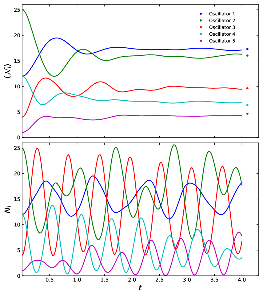
A broadly relevant question is the following: over what time scale is a classical description of a highly degenerate but self-interacting Bosonic system valid? We call that time scale the duration of classicality of the system. Two of us (PS and ET) have recently [25] addressed this by numerically integrating the equations of motion of a toy model consisting of five interacting quantum oscillators. In all the cases simulated, the duration of classicality was found to be shorter or at most of order the thermal relaxation time $\tau$ . A summary of the results of ref. [25] is included in subsection II.2. We add however new simulations in which only one of the five oscillators is excited in the initial state. According to its classical evolution, this state persists forever. According to its quantum evolution, the state has a finite lifetime because the quanta jump out of the initially excited oscillator into the four others. The new simulations parallel our analytical treatment of the homogeneous condensate with attractive contact interactions in Section III and of the homogeneous self-gravitating condensate in critical expansion in Section IV.

In Section III we develop a formalism to help calculate the quantum evolution of a scalar field that is described in its initial state by a classical solution. A classical solution corresponds to one mode of the quantum field. In the initial state all quanta are placed into that single mode. However the quantum field has an infinite number of other modes. We expand the quantum field into a complete orthonormal set of modes built around an arbitrary classical solution. We derive the Hamiltonian in terms of the associated creation and annihilation operators. The formalism is applicable to any condensate described by a classical solution.

We first apply the formalism to the homogeneous condensate in $\lambda\phi^{4}$ theory, with $\lambda>0$ and $\lambda<0$ , in Section III. The condensate is unstable when $\lambda<0$ . Nonetheless, in its classical description, the homogeneous condensate persists forever. In its quantum description, the homogeneous condensate is depleted by parametric resonance. We obtain the time scale over which the condensate is depleted, which is in effect its duration of classicality. In Section IV we apply the formalism to a homogeneous self-gravitating condensate in critical expansion. Again, in its classical description, the condensate persists forever whereas it is depleted by parametric resonance in its quantum description. Here too we derive the time scale over which the condensate is depleted, and after which a classical description is invalid. In the self-gravity case, the instability grows as a power of time whereas it grows exponentially fast in $\lambda\phi^{4}$ theory with $\lambda<0$ . The results we derive in Section III and IV are all exact statements in the limit where the number of quanta $N$ in the condensate is very large compared to the number of quanta not in the condensate.

Although we only analyze the behaviour of homogeneous condensates in this paper, we expect our conclusions to apply to inhomogeneous condensates as well. Indeed, a homogeneous condensate can be seen as a limiting case of inhomogeneous condensates. Since homogeneous condensates are depleted by parametric resonance, the same must be true for inhomogeneous condensates, at least in the limit of small deviations away from homogeneity. In fact in our simulations of the five oscillator toy model we find that the condensates which persist forever according to their classical evolution are the condensates with the longest duration of classicality in their quantum evolution. We explain this result on the basis of analytical arguments. By analogy, we expect inhomogeneous condensates to have shorter durations of classicality than homogeneous ones.

Related topics were discussed in two recent papers [26, 27]. Inter alia, ref. [26] solves the classical equations of motion for an initially almost homogeneous condensate with attractive contact interactions numerically on a lattice. If it were strictly homogeneous, the condensate would persist forever. Perturbations are introduced to mimick quantum fluctuations. As the perturbations grow, the condensate is depleted in a manner which is qualitatively consistent with our quantum field theory treatment. Ref. [27] discusses, as we do, the duration of classicality of the cosmic axion fluid. The conclusions of ref. [27] differ from ours.

A brief outline of our paper is as follows. In Section II, we discuss Bose-Einstein condensation and analyze four issues which may cause confusion when the interactions are attractive, as is the case for dark matter axions. In Section III, we introduce a formalism to calculate in quantum field theory the departures from a description of a system by classical field equations. We apply it to the homogeneous condensate in $\lambda\phi^{4}$ theory in the repulsive ( $\lambda>0$ ) and attractive ( $\lambda<0$ ) cases. In Section IV, we apply the formalism to a homogeneous self-gravitating condensate in critical expansion. In Section V, we summarize our conclusions.

II Bose-Einstein condensation

This section gives a brief description of the phenomenon of Bose-Einstein condensation, emphasizing the necessary and sufficient conditions for its occurrence, and the reason why it occurs. We follow this with a discussion of four subtopics which appear occasionally to cause confusion in discussions of Bose-Einstein condensation of dark matter axions.

Consider a system of $N$ identical bosons in thermal equilibrium under the constraint that the total number of particles is conserved. A standard textbook derivation yields the average occupation number $\langle{\cal N}_{j}\rangle$ of particle state $j$ in the limit of a huge number of particles (the so-called thermodynamic limit):

\langle{\cal N}_{j}\rangle={1\over e^{{1\over T}(\epsilon_{j}-\mu)}-1}

(1)

where $T$ is the temperature, $\mu$ the chemical potential, and $\epsilon_{j}$ ( $j=0,1,2,3...$ ) the energy of particle state $j$ . We will assume that the particle states are ordered so that $\epsilon_{0}<\epsilon_{1}<\epsilon_{2}<...~$ . The $\langle{\cal N}_{j}\rangle$ maximize the system entropy for a given total energy $E=\sum_{j}{\cal N}_{j}\epsilon_{j}$ and total number of particles $N=\sum_{j}{\cal N}_{j}$ . Since all $\langle{\cal N}_{j}\rangle\geq 0$ , it is necessary that $\mu<\epsilon_{0}$ for Eq. (1) to make sense. On the other hand, the total number of particles $N(T,\mu)=\sum_{j}\langle{\cal N}_{j}\rangle$ is an increasing function of $\mu$ for fixed $T$ since each $\langle{\cal N}_{j}\rangle$ is. So, if $N$ is increased while $T$ is held fixed, $\mu$ must increase but it can not become larger than $\epsilon_{0}$ . In the systems of interest to us, the total number of particles in excited ( $j>0$ ) states has for $\mu=\epsilon_{0}$ a finite value

N_{\rm ex}(T,\mu=\epsilon_{0})=\sum_{j>0}{1\over e^{{1\over T}(\epsilon_{j}-\epsilon_{0})}-1}~~\ .

(2)

(In one and two spatial dimensions, $N_{\rm ex}(T,\mu=\epsilon_{0})$ may be infinite because of an infrared divergence but this comment is not relevant to the systems in three spatial dimensions that interest us.) Consider what happens when, at fixed $T$ , $N$ is made larger than $N_{\rm ex}(T,\mu=\epsilon_{0})$ . The only possible system response is for the extra $N-N_{\rm ex}(T,\mu=\epsilon_{0})$ particles to go to the ground state ( $j=0$ ). Indeed the average occupation number $\langle{\cal N}_{0}\rangle$ of that state becomes arbitrarily large as $\mu$ approaches $\epsilon_{0}$ from below.

From the above we deduce four conditions for Bose-Einstein condensation: i) the system comprises a large number of identical bosons, hereafter called particles for short, ii) the number of particles is conserved, iii) the particles are sufficiently degenerate, and iv) the particles are in thermal equilibrium. The number of particles has to be sufficiently large (condition i) for the system to be in the thermodynamic limit. The number of particles has to be conserved (condition ii) but only on the time scale of thermalization. It need not be absolutely conserved. For example, it is irrelevant to Bose-Einstein condensation in dilute gases whether baryons are absolutely stable. The only thing that matters is that they are stable on the time scale of the condensation process. (Whether they decay tomorrow is irrelevant to their condensation this minute.) Dark matter axions are not absolutely stable since they decay to two photons. However their lifetime is much longer than the age of the universe and so is the timescale of all other axion number changing processes. Condition iii) is satisfied if the degeneracy, i.e. the average occupation number $\langle{\cal N}_{j}\rangle$ of those states that are occupied, is larger than some critical number of order one. For systems in thermal equilibrium this condition is the requirement that the temperature is lower than some critical temperature. The critical temperature is such that the interparticle distance is of order the thermal de Broglie wavelength. Thermal equilibrium is generally taken for granted in discussions of Bose-Einstein condensation in liquid ⁴He and dilute gases because these systems thermalize very quickly. For these systems, condition iv) is readily satisfied but condition iii) is difficult to achieve because of the low temperatures required. The reverse situation pertains to dark matter axions. Axions thermalize only very slowly, perhaps on the timescale of the age of the universe, or not at all, because axions are very weakly interacting. On the other hand, their quantum degeneracy is enormous with ${\cal N}\sim 10^{61}$ . For these reasons we state condition iii) independently and ahead of condition iv).

Thermalization involves interactions and requires time. We define the relaxation time $\tau$ to be the time scale over which the distribution $\{{\cal N}_{j}\}$ of the particles over the particle states changes completely, each ${\cal N}_{j}$ changing by order 100%. Whether condition iv) for Bose-Einstein condensation is satisfied is an issue of time scales. Let us assume that the first three conditions are satisfied and that the system is out of equilibrium, i.e. the system is in a state of entropy less than allowed. The system will then thermalize on the time scale $\tau$ , increasing its entropy. It forms a BEC because the state of highest entropy, given that the first three conditions are satisfied, is one in which a fraction of order one of the particles is in the lowest energy available state and the remaining particles in a thermal distribution in excited states. The entropy increases when a BEC forms. The process is irreversible.

We now discuss four aspects of Bose-Einstein condensation that appear sometimes to be sources of confusion in the literature, and must be clarified especially in the context of cosmic axion Bose-Einstein condensation.

II.0.1 Quantum mechanics is essential

It is possible within classical field theory to produce a phenomenon similar to Bose-Einstein condensation by introducing a cutoff $k_{\rm UV}$ on the wavevectors of the field modes. Indeed the classical physics analog of Eq. (1) is

\langle{\cal N}_{j}\rangle={T\over\epsilon_{j}-\mu}~~\ .

(3)

When $\mu$ approaches $\epsilon_{0}$ from below, provided $T\neq 0$ , $\langle{\cal N}_{0}\rangle$ diverges as it does for the Bose-Einstein distribution. However in classical field theory the energy gets distributed equally over all field modes. If there is no cutoff the specific heat per unit volume diverges because, in any finite volume, the field has an infinite number of modes with large wavevectors $\vec{k}$ . In other words, $T=0$ in any finite volume containing finite energy in thermal equilibrium.

To produce a phenomenon resembling Bose-Einstein condensation in classical field theory, a cutoff is introduced by hand with value fixed so that

T_{\rm crit}\sim{k_{\rm UV}^{2}\over 2m}

(4)

where $m$ is the boson mass and $T_{\rm crit}$ the critical temperature that is naturally present in the quantum theory. The number of modes per unit volume is finite then, of order $k_{\rm UV}^{3}/(2\pi)^{3}$ . As a result $T\neq 0$ in the cutoff field theory and ${\cal N}_{0}\rightarrow\infty$ when $\mu$ approaches $\epsilon_{0}$ from below. However, this does not mean that the cutoff classical field theory has any validity beyond producing some form of Bose-Einstein condensation. The cutoff is not meant to be present in any real sense. In general the cutoff classical field theory differs from the quantum field theory, and when the two make different predictions it is the latter that is to be believed not the former. In particular, as discussed in ref. [20], the classical theory conserves vorticity, i.e. the circulation of the velocity field along a closed path $\Gamma$

{\cal C}[\Gamma]\equiv\oint_{\Gamma}~d\vec{r}\cdot\vec{v}(\vec{r},t)~~\ ,

(5)

whereas the quantum theory does not. Conservation of vorticity in classical field theory follows from the continuity and single-valuedness of the wavefunction, and holds whether or not a wavevector cutoff is introduced. In contrast, vorticity is not conserved in the quantum field theory because quanta can jump between modes of different vorticity. The creation of vorticity is essential to explain the phenomenology of caustic rings and solve the galactic angular momentum problem [20].

It is pertinent, we believe, to remark that Eq. (4) does not make sense unless a quantity with dimension of action, such as $\hbar$ , is introduced by hand. The classical field theory does not have a notion of particles nor therefore of particle mass, even after the wavevector cutoff $k_{\rm UV}$ has been introduced. It has only modes with dispersion law

\omega(\vec{k})=\sqrt{\omega_{0}^{2}+c^{2}\vec{k}\cdot\vec{k}}

(6)

where $\omega_{0}$ is the angular frequency of oscillation of the $\vec{k}=0$ mode. In the quantum theory, the particle mass is given by

m=\omega_{0}\hbar/c^{2}

(7)

but in the classical theory, with or without cutoff, there is no such thing as particle mass. Likewise, Eq. (4) should be written

T_{\rm crit}\sim{(\hbar k_{\rm UV})^{2}\over 2m}

(8)

to be dimensionally consistent.

II.0.2 How long is a classical description valid?

Granted that the outcome of thermalization in a degenerate Bosonic system is different from that of its classical analog, one may still ask how long a classical description of such a system is accurate. This question was the topic of a recent paper by two of us [25], in which it was shown by analytical arguments and numerical simulation of a toy model that the duration of classicality of a degenerate interacting Bosonic system is of order, and not longer than, its thermalization time $\tau$ . We summarize some results of ref. [25] here, and add toy model simulations that are analogous to our analytical calculations in Sections III and IV.

A general Bosonic system that conserves the number of quanta has a Hamiltonian of the form

H=\sum_{j}\omega_{j}a_{j}^{\dagger}a_{j}+{1\over 4}\sum_{jkln}\Lambda_{jk}^{ln}a_{j}^{\dagger}a_{k}^{\dagger}a_{l}a_{n}

(9)

where the $a_{j}$ and $a_{j}^{\dagger}$ are annihilation and creation operators satisfying canonical equal-time commutation relations. One might add to the RHS of Eq. (9) terms of the form $a^{\dagger}a^{\dagger}a^{\dagger}a~a~a$ , and so forth, but this would not alter the discussion in a significant way. ${\cal N}_{j}=a_{j}^{\dagger}a_{j}$ is the number of quanta in oscillator $j$ . In the Heisenberg picture, the annihilation operators $a_{j}(t)$ satisfy the equations of motion

i\dot{a}_{j}=[a_{j},H]=\omega_{j}a_{j}+{1\over 2}\sum_{kln}\Lambda_{jk}^{ln}a_{k}^{\dagger}a_{l}a_{n}~~\ .

(10)

The classical description of the system is obtained by replacing the $a_{j}(t)$ with c-numbers $A_{j}(t)$ . They satisfy

i\dot{A}_{j}=\omega_{j}A_{j}+{1\over 2}\sum_{kln}\Lambda_{jk}^{ln}A_{k}^{*}A_{l}A_{n}~~\ .

(11)

The classical analogs of the quantum state occupation numbers ${\cal N}_{j}$ are $N_{j}=A_{j}^{*}A_{j}$ . The question is: given the same initial values, how long do the classical analogs $N_{j}(t)$ track the expectation values $<{\cal N}_{j}(t)>$ of the quantum operators? We call ”duration of classicality” the time scale over which the classical description accurately describes the quantum system within some margin of error, say 20%.

To address this issue, a toy model of five quantum oscillators was simulated numerically [25]. The toy model had been previously discussed and simulated in ref. [10] to verify numerically the validity of formulae that estimate the rate of thermalization in the ’condensed regime’, defined by the condition $\Gamma>\delta\epsilon$ where $\Gamma$ is the thermalization rate and $\delta\epsilon$ the energy dispersion of the quanta in the system. The dark matter axion fluid thermalizes in the condensed regime. The Hamiltonian of the toy model has the form given in Eq. (9) with $\omega_{j}=j\omega_{1}$ ( $j$ = 1, 2, 3, 4, 5) and $\Lambda_{jk}^{ln}=0$ unless $j+k=l+n$ . Non-zero values are given to $\Lambda_{14}^{23}$ , $\Lambda_{15}^{24}$ , $\Lambda_{25}^{34}$ , $\Lambda_{22}^{13}$ , $\Lambda_{33}^{24}$ , $\Lambda_{33}^{15}$ and $\Lambda_{44}^{35}$ , and their conjugates $\Lambda_{jk}^{ln}=\Lambda_{ln}^{jk~*}$ . The Schrödinger equation

i\partial_{t}|\Psi(t)\rangle=H|\Psi(t)\rangle

(12)

was solved numerically for a large variety of initial conditions. In all cases it was found that the duration of classicality is less than or at most of order the relaxation time $\tau$ , defined as the time scale over which the distribution of the quanta over the oscillators changes completely. Fig. 1 shows in its top panel the quantum evolution of the initial state $|{\cal N}_{1},{\cal N}_{2},...,{\cal N}_{5}\rangle=|12,25,4,12,1\rangle$ as an example. The figure shows that the expectation values $\langle{\cal N}_{j}\rangle$ move towards their thermal averages on the expected time scale $\tau=1/\Gamma$ , which is of order 0.4 given the coupling strengths $\Lambda_{jk}^{ln}$ in the simulation [10]. The thermal averages are shown by the dots on the right side of Fig. 1 (top panel). The bottom panel of Fig. 1 shows the classical evolution of the initial state $(A_{1},A_{2},...,A_{5})=(\sqrt{12},\sqrt{25},\sqrt{4},\sqrt{12},\sqrt{1})$ , in which the $N_{j}$ and their time derivatives $\dot{N}_{j}$ have the same initial values as their quantum analogues in the top panel. Fig. 1 shows that the classical evolution tracks the quantum evolution only for a time of order, and relatively short compared to, $\tau$ .

The toy model can be made to behave analogously to the homogeneous quantum field condensates discussed in Section III and IV. The homogeneous condensates persist indefinitely in their classical description but have a finite lifetime in their quantum description. Initial states with the analogous property in the toy model are $|0,N,0,0,0\rangle$ . In their classical evolution, these states persist indefinitely because the RHS of Eq. (11) vanishes. In their quantum evolution, the quanta in the 2nd oscillator jump in pairs to the 1st and 3rd oscillators and thence to the 4th and 5th oscillators. Fig. 2 shows the $\langle{\cal N}_{j}(t)\rangle$ as a function of time for $N=100$ in panel a), contrasted with the constant $N_{j}$ in panel b). For the generic initial states simulated in ref. [25], the relaxation rate is of order $\Gamma\sim\Lambda\sqrt{I}{\cal N}$ for both the classical and quantum evolutions, where $I$ is the number of relevant interaction terms on the RHS of Eq. (9), and $\Lambda$ and ${\cal N}$ are typical values of the interaction strengths and of the quantum occupation numbers [10]. For the special initial states $|0,N,0,0,0\rangle$ the relaxation rate vanishes according to the classical evolution but is of order $\Gamma\sim|\Lambda_{13}^{22}|N/\log(N)$ according to the quantum evolution. The factor $\log(N)$ appears because the relaxation of these special states is limited by the initial process 2 + 2 $\rightarrow$ 1 + 3, which acts as a bottleneck. The 2 + 2 $\rightarrow$ 1 + 3 process causes the occupation numbers of the 1st and 3d oscillators to grow as $e^{|\Lambda_{13}^{22}|Nt}$ , the difference between the classical and quantum evolutions being only that the growth is seeded in the quantum evolution whereas it is unseeded in the classical evolution. Applying the methods of Section III and IV to the toy model, one finds

\langle{\cal N}_{1}\rangle=\langle{\cal N}_{3}\rangle=\sinh^{2}(\gamma t)

(13)

with $\gamma={1\over 2}|\Lambda_{13}^{22}|N$ , and therefore

\langle{\cal N}_{2}\rangle=N-2~\sinh^{2}(\gamma t)

(14)

for $t$ sufficiently small that the condensate has not been depleted much yet. The dotted lines in Fig. 2 show $\langle{\cal N}_{2}(t)\rangle$ , $\langle{\cal N}_{1}(t)\rangle$ and $\langle{\cal N}_{3}(t)\rangle$ according to Eqs. (13) and (14). The behavior of our toy model condensate is consistent with the discussion of a similar toy model condensate in ref. [28].

In summary, the duration of classicality of the initial state $|0,N,0,0,0\rangle$ , which persists indefinitely according to its classical evolution, is a factor $\log(N)$ longer than the duration of classicality of generic states $|{\cal N}_{1},{\cal N}_{2},{\cal N}_{3},{\cal N}_{4},{\cal N}_{5}\rangle$ . The $|0,N,0,0,0\rangle$ state is the toy model analog of the homogeneous condensates discussed in Sections III and IV. Those homogeneous condensates also persist forever according to their classical evolution, but have a finite duration of classicality according to their quantum evolution. We expect the duration of classicality of inhomogeneous condensates to be shorter than that of homogeneous condensates for the same reason that the duration of classicality of generic toy model initial states is shorter than that of the $|0,N,0,0,0\rangle$ initial state, the reason being the absence in the case of generic states of the thermalization bottleneck that is present for the initial state $|0,N,0,0,0\rangle$ .

II.0.3 Homogeneity is not a necessary outcome, or criterion

Contrary to statements appearing occasionally in the literature, the condensed state need not be a state of momentum $\vec{p}=0$ . Generally, it is not. The state $\vec{p}=0$ is homogeneous and minimizes the kinetic energy $\omega_{\vec{p}}={\vec{p}\cdot\vec{p}\over 2m}$ of a particle in empty space. But in general 1) space is not empty and 2) the particle energies $\epsilon_{j}$ that appear in Eq. (1) differ from the frequencies $\omega_{j}$ that appear in Eq. (9) because of interactions. Even in empty space, the lowest energy available state need not be the zero momentum state.

Lack of homogeneity is no impediment to Bose-Einsten condensation. Fig. 3 shows a Bose-Einstein condensate that is highly inhomogeneous on some length scale $d$ but extends over a much larger length scale $L$ . It may be realized by placing superfluid ⁴He in a long tube with various obstructions on the length scale $d$ inside the tube. Although inhomogeneous on the length scale $d$ the condensate has long range correlations on the length scale $L$ , as we now show explicitly.

For a general system undergoing Bose-Einstein condensation, let $u^{j}(\vec{x},t)$ be the wavefunction of the particle state with energy $\epsilon_{j}$ . The wavefunctions form a complete orthonormal set:

	$\displaystyle\int_{V}d^{3}x~u^{j}(\vec{x},t)^{*}~u^{k}(\vec{x},t)$	$\displaystyle=$	$\displaystyle\delta^{k}_{j}$
	$\displaystyle\sum_{j}u^{j}(\vec{x},t)^{*}~u^{j}(\vec{y},t)$	$\displaystyle=$	$\displaystyle\delta(\vec{x}-\vec{y})~~\ .$		(15)

The quantum scalar field $\phi(\vec{x},t)$ describing the particles undergoing Bose-Einstein condensation and its canonically conjugate field $\pi(\vec{x},t)$ may be expanded in terms of those wavefunctions:

	$\displaystyle\phi(\vec{x},t)$	$\displaystyle=$	$\displaystyle\sum_{j}{1\over\sqrt{2m}}[u^{j}(\vec{x},t)b_{j}(t)+u^{j}(\vec{x},t)^{*}b_{j}(t)^{\dagger}]$
	$\displaystyle\pi(\vec{x},t)$	$\displaystyle=$	$\displaystyle\sum_{j}\sqrt{m\over 2}{1\over i}[u^{j}(\vec{x})b_{j}(t)-u^{j}(\vec{x},t)^{*}b_{j}(t)^{\dagger}]$		(16)

where the $b_{j}(t)$ and $b_{j}^{\dagger}(t)$ are annihilation and creation operators satisfying canonical equal time commutation relations. Note that the $b_{j}(t)$ and $b_{j}^{\dagger}(t)$ in Eq. (16) are different from the $a_{j}(t)$ and $a_{j}^{\dagger}(t)$ in the previous subsection since the latter annihilate and create particles in eigenstates of the free Hamiltonian, whereas the $b_{j}(t)$ and $b_{j}^{\dagger}(t)$ annihilate and create particles in eigenstates of the one-particle Hamiltonian in which the interactions of the one particle with all the other particles are derived from the full Hamiltonian using mean field theory.

A general system state may be written

|\Psi\rangle=\sum_{\{{\cal N}_{j}\}}c(\{{\cal N}_{j}\})|\{{\cal N}_{j}\}\rangle_{t}

(17)

where $\{{\cal N}_{j}\}$ is an arbitrary distribution of the occupation numbers over the particle states,

|\{{\cal N}_{j}\}\rangle_{t}=\prod_{j}{1\over\sqrt{{\cal N}_{j}!}}(b_{j}(t)^{\dagger})^{{\cal N}_{j}}|0\rangle

(18)

and $|0\rangle$ is the empty state. Since the total number of particles is conserved, we may take $|\Psi\rangle$ to be an eigenstate of the total number operator

\sum_{j}b_{j}(t)^{\dagger}b_{j}(t)|\Psi\rangle=N|\Psi\rangle~~\ ,

(19)

in which case, $c(\{{\cal N}_{j}\})=0$ unless $\sum_{j}{\cal N}_{j}=N$ . In the state $|\Psi\rangle$ , the field $\phi(\vec{x},t)$ has equal-time correlation function

	$\displaystyle\langle\Psi\|\phi(\vec{x},t)\phi(\vec{y},t)\|\Psi\rangle=\sum_{\{{\cal N}_{j}\}}\sum_{\{{\cal N}_{j}^{\prime}\}}c^{*}(\{{\cal N}_{j}\})c(\{{\cal N}_{j}^{\prime}\})\sum_{k,l}{1\over 2m}\cdot$	(20)
$\displaystyle\cdot$	$\displaystyle\big[u^{k}(\vec{x},t)^{*}u^{l}(\vec{y},t)~_{t}\langle\{{\cal N}_{j}\}\|b_{k}^{\dagger}(t)b_{l}(t)\|\{{\cal N}_{j}^{\prime}\}\rangle_{t}$
$\displaystyle+$	$\displaystyle~u^{k}(\vec{x},t)u^{l}(\vec{y},t)^{*}~_{t}\langle\{{\cal N}_{j}\}\|b_{k}(t)b_{l}^{\dagger}(t)\|\{{\cal N}_{j}^{\prime}\}\rangle_{t}\big]~\ .$

If a Bose-Einstein condensate has formed, the lowest energy available state has occupation number $N_{0}$ of order $N$ . In that case $c(\{{\cal N}_{j}\})=0$ unless ${\cal N}_{0}\simeq N_{0}$ and therefore

\langle\Psi|\phi(\vec{x},t)\phi(\vec{y},t)|\Psi\rangle={N_{0}\over 2m}(u^{0}(\vec{x},t)^{*}u^{0}(\vec{y},t)+u^{0}(\vec{x},t)u^{0}(\vec{y},t)^{*})~+~...

(21)

where the dots are contributions, from particle states other than the condensed state, that fall off exponentially or as a power law with distance $|\vec{x}-\vec{y}|\equiv r$ . The contribution from the condensed state does not fall with distance $r$ . Instead, for given $\vec{y}$ , it has support wherever $u^{0}(\vec{x},t)$ has support. Thus any Bose-Einstein condensate is correlated over the whole extent of the condensate.

II.0.4 What state do the particles condense into?

Since thermalization is a condition for Bose-Einstein condensation, it follows that the state the particles condense into is the lowest energy state that is available to them through the thermalizing interactions. In general it is not the lowest energy state in an absolute sense. For example, if a beaker of superfluid ⁴He sits on a table, a macroscopically large number of atoms are in a condensed state. This condensed state is certainly not the lowest energy state since its energy can be lowered by placing the beaker on the floor. It is, however, the lowest energy state available to the ⁴He atoms through the thermalizing interactions.

As was already mentioned, the condensed state need not be stable. Ideally, however, it ought to be stable on the thermalization time scale. A complicating factor is that thermalization is rarely complete. Fortunately, Bose-Einstein condensation occurs immediately and explosively on the thermalization time scale. The rate at which particles move to the condensed state is proportional to the number of particles that are already in the condensed state [29]. The time scale over which a complete Bose-Einstein distribution is established is generally much longer than the time scale over which the Bose-Einstein condensate forms [12].

Nonetheless, in the case of Bose-Einstein condensation of dark matter axions, we have to deal with the complication that the axion fluid is made unstable by the very interaction that thermalizes it. After Bose-Einstein condensation has occurred, further thermalization is required because the instability causes the lowest energy available state to change with time. Our paper is motivated by the question what is the outcome of thermalization while density perturbations grow and how does this outcome differ from the predictions of cosmological perturbation theory with ordinary CDM.

In the remainder of this paper we construct a formalism that allows one to discuss more clearly the thermalization of a fluid made unstable, and therefore inhomogeneous, by the very interactions that thermalize it. In Section III, we discuss the evolution of a highly degenerate Bose fluid with attractive $\lambda\phi^{4}$ interactions $(\lambda<0$ ). In Section IV, we discuss the evolution of a highly degenerate Bose fluid with gravitational self-interactions. We discuss the $\lambda\phi^{4}$ case first because it is somewhat simpler.

III Attractive contact interactions

In this section, we introduce a formalism to analyze the thermalization and evolution of a highly degenerate Bose fluid with attractive contact interactions. The interactions play the double role of rendering the fluid unstable and of thermalizing it. This section is mainly a warmup exercise preliminary to analyzing the thermalization and evolution of a highly degenerate Bose fluid with gravitational self-interactions in the next section. It may also be useful in the analysis of some condensed matter systems.

The model we analyze is $\lambda\phi^{4}$ theory. Its Hamiltonian is

H=\int d^{3}x[{1\over 2}(\pi)^{2}+{1\over 2}(\vec{\nabla}\phi)^{2}+{1\over 2}m^{2}\phi^{2}+{\lambda\over 4!}:\phi^{4}:]

(22)

where $\phi(\vec{x},t)$ and $\pi(\vec{x},t)$ are conjugate Hermitian scalar fields satisfying canonical equal time commutation relations. The double colon $:...:$ symbol in the last term of Eq. (22) indicates normal ordering. That term describes contact interactions. They are repulsive if $\lambda>0$ and attractive if $\lambda<0$ . The $\phi$ and $\pi$ fields satisfy the equations of motion

\partial_{t}\phi=\pi~~~,~~~~\partial_{t}\pi-\nabla^{2}\phi+m^{2}\phi+{\lambda\over 6}:\phi^{3}:~=0~~~\ .

(23)

We will concern ourselves only with the non-relativistic regime of the theory. The non-relativistic limit is obtained by setting

	$\displaystyle\phi(\vec{x},t)$	$\displaystyle=$	$\displaystyle{1\over\sqrt{2m}}[\psi(\vec{x},t)e^{-imt}+\psi(\vec{x},t)^{\dagger}e^{imt}]$
	$\displaystyle\pi(\vec{x},t)$	$\displaystyle=$	$\displaystyle\sqrt{m\over 2}(-i)[\psi(\vec{x},t)e^{-imt}-\psi(\vec{x},t)^{\dagger}e^{imt}]~~\ ,$		(24)

neglecting terms of order $\partial_{t}\psi$ versus terms of order $m\psi$ , and ignoring terms proportional to $e^{2imt}$ and $e^{-2imt}$ that oscillate so fast in time that they effectively average to zero. $\psi(\vec{x},t)$ is a non-Hermitian scalar field satisfying the equal time commutation relations

[\psi(\vec{x},t),\psi(\vec{y},t)]=0~~~~,~~~~[\psi(\vec{x},t),\psi(\vec{y},t)^{\dagger}]=\delta^{3}(\vec{x}-\vec{y})~~~\ ,

(25)

and the equation of motion

i\partial_{t}\psi=-{1\over 2m}\nabla^{2}\psi+{\lambda\over 8m^{2}}\psi^{\dagger}\psi~\psi~~\ .

(26)

Note that the number of particles is conserved in the non-relativistic limit even though the number of particles is not conserved in the original theory, Eq. (22).

We expand the $\psi$ field

\psi(\vec{x},t)=\sum_{\vec{\alpha}}u^{\vec{\alpha}}(\vec{x},t)a_{\vec{\alpha}}(t)

(27)

in an orthonormal and complete set of wavefunctions $u^{\vec{\alpha}}(\vec{x},t)$ , labeled by $\vec{\alpha}$ . Thus

	$\displaystyle\int_{V}d^{3}x~u^{\vec{\alpha}}(\vec{x},t)^{*}u^{\vec{\beta}}(\vec{x},t)$	$\displaystyle=$	$\displaystyle\delta_{\vec{\alpha}}^{\vec{\beta}}~~~{\rm and}$
	$\displaystyle\sum_{\vec{\alpha}}u^{\vec{\alpha}}(\vec{x},t)^{*}u^{\vec{\alpha}}(\vec{y},t)$	$\displaystyle=$	$\displaystyle\delta^{3}(\vec{x}-\vec{y})$		(28)

where $V$ is the volume of space where the theory is defined. The $a_{\vec{\alpha}}(t)$ and $a_{\vec{\alpha}}(t)^{\dagger}$ are annihilation and creation operators satisfying equal time commutation relations

[a_{\vec{\alpha}}(t),a_{\vec{\beta}}(t)]=0~~~,~~~[a_{\vec{\alpha}}(t),a_{\vec{\beta}}(t)^{\dagger}]=\delta_{\vec{\alpha}}^{\vec{\beta}}~~~\ ,

(29)

and the equation of motion

i\partial_{t}a_{\vec{\alpha}}=\sum_{\vec{\beta}}M_{\vec{\alpha}}^{\vec{\beta}}a_{\vec{\beta}}~+~{1\over 2}\sum_{\vec{\beta},\vec{\gamma},\vec{\delta}}\Lambda_{\vec{\alpha}\vec{\beta}}^{\vec{\gamma}\vec{\delta}}~a_{\vec{\beta}}^{\dagger}a_{\vec{\gamma}}a_{\vec{\delta}}

(30)

with

	$\displaystyle M_{\vec{\alpha}}^{\vec{\beta}}(t)$	$\displaystyle=$	$\displaystyle\int_{V}d^{3}x~u^{\vec{\alpha}}(\vec{x},t)^{*}(-i\partial_{t}-{1\over 2m}\nabla^{2})u^{\vec{\beta}}(\vec{x},t)$
	$\displaystyle\Lambda_{\vec{\alpha}\vec{\beta}}^{\vec{\gamma}\vec{\delta}}(t)$	$\displaystyle=$	$\displaystyle{\lambda\over 4m^{2}}\int_{V}d^{3}x~u^{\vec{\alpha}}(\vec{x},t)^{}u^{\vec{\beta}}(\vec{x},t)^{}u^{\vec{\gamma}}(\vec{x},t)u^{\vec{\delta}}(\vec{x},t)~~~\ .$		(31)

In the non-relativistic limit, the above equations are exact for any orthonormal complete set of states $u^{\vec{\alpha}}$ .

III.1 Classical description

The classical description is obtained by replacing the quantum field $\psi(\vec{x},t)$ by a wavefunction $\Psi(\vec{x},t)$ . $\Psi$ satisfies the c-number version of Eq. (26)

i\partial_{t}\Psi=-{1\over 2m}\nabla^{2}\Psi+{\lambda\over 8m^{2}}|\Psi|^{2}\Psi

(32)

called the Schrödinger-Gross-Pitaevskii equation. (Although wavefunctions are historically associated with a quantum mechanical description, from the point of view of quantum field theory a wavefunction is merely a solution of the classical field equations in the non-relativistic limit.) The wavefunction may be written

\Psi(\vec{x},t)=A(\vec{x},t)e^{i\beta(\vec{x},t)}~~\ ,

(33)

where $A(\vec{x},t)$ and $\beta(\vec{x},t)$ are real. The wavefunction $\Psi$ describes a fluid of number density

n(\vec{x},t)=A(\vec{x},t)^{2}

(34)

and velocity

\vec{v}(\vec{x},t)={1\over m}\vec{\nabla}\beta(\vec{x},t)~~\ .

(35)

Eq. (32) implies the continuity equation

\partial_{t}n+\vec{\nabla}\cdot(n\vec{v})=0

(36)

and the Euler-like equation

\partial_{t}\vec{v}+(\vec{v}\cdot\vec{\nabla})v=-{1\over m}\vec{\nabla}V-\vec{\nabla}q

(37)

where

V(\vec{x},t)={\lambda\over 8m^{2}}n(\vec{x},t)

(38)

and

q(\vec{x},t)=-{1\over 2m^{2}}{\nabla^{2}\sqrt{n}\over\sqrt{n}}~~\ .

(39)

$q(\vec{x},t)$ is sometimes called “quantum pressure”. Except for the $-\vec{\nabla}q$ term, Eq. (37) is the Euler equation for a fluid of classical particles moving in the potential $V$ . The $-\vec{\nabla}q$ term is a consequence of the underlying wave nature of the fluid and accounts, for example, for the tendency of a wavepacket to spread.

Eq. (32) admits the homogeneous solution

\Psi_{0}=\sqrt{n_{0}}e^{-i\delta\omega t}

(40)

where

\delta\omega={\lambda n_{0}\over 8m^{2}}~~\ .

(41)

Consider small perturbations about that solution

\Psi(\vec{x},t)=\Psi_{0}(t)~+~\Psi_{1}(\vec{x},t)~~\ .

(42)

To lowest order, the perturbations satisfy

i\partial_{t}\Psi_{1}=-{1\over 2m}\nabla^{2}\Psi_{1}+\delta\omega(2\Psi_{1}+e^{-2i\delta\omega t}\Psi_{1}^{*})~~\ .

(43)

We decompose the perturbation in Fourier modes as follows

\Psi_{1}(\vec{x},t)=e^{-i\delta\omega t}\sum_{\vec{k}}C_{\vec{k}}(t)e^{i\vec{k}\cdot\vec{x}}~~\ .

(44)

The Fourier amplitudes satisfy

i\partial_{t}C_{\vec{k}}(t)=({k^{2}\over 2m}+\delta\omega)C_{\vec{k}}(t)+\delta\omega C_{-\vec{k}}(t)^{*}~~\ .

(45)

The solutions may be written

C_{\vec{k}}(t)=s_{\vec{k}}(t)+r_{\vec{k}}(t)

(46)

with

s_{-\vec{k}}(t)^{*}=s_{\vec{k}}(t)~~~{\rm and}~~~r_{-\vec{k}}(t)^{*}=-r_{\vec{k}}(t)~~\ .

(47)

Eqs. (45) imply that

r_{\vec{k}}(t)={2mi\over k^{2}}\partial_{t}s_{\vec{k}}(t)

(48)

and that $s_{\vec{k}}(t)$ is a solution of

\partial_{t}^{2}~s_{\vec{k}}(t)=-{k^{2}\over 2m}({k^{2}\over 2m}+2\delta\omega)s_{\vec{k}}(t)~~\ .

(49)

We now discuss the repulsive ( $\lambda>0$ ) and attractive ( $\lambda<0$ ) cases separately.

For $\lambda>0$ , the perturbations oscillate with angular frequency

\omega(k)=\sqrt{{k^{2}\over 2m}({k^{2}\over 2m}+{\lambda n_{0}\over 4m^{2}})}~~~\ .

(50)

For long wavelengths, i.e. $k<<k_{c}\equiv{\sqrt{\lambda n_{0}\over 2m}}$ , the dispersion law is linear

\omega(k)=v_{s}k

(51)

with sound speed

v_{s}=\sqrt{\lambda n_{0}\over 8m^{3}}~~\ ,

(52)

whereas for short wavelengths ( $k>>k_{c}$ ) the dispersion law is quadratic. The most general solution to Eq. (43) is Eq. (44) with

C_{\vec{k}}(t)=c_{\vec{k}}({k^{2}\over 2m}+\omega(k))e^{-i\omega(k)t}+c_{-\vec{k}}^{*}({k^{2}\over 2m}-\omega(k))e^{i\omega(k)t}

(53)

where the $c_{\vec{k}}$ are complex numbers which can be determined in terms of the initial perturbation $\Psi_{1}(\vec{x},0)$ .

In the attractive case ( $\lambda=-|\lambda|$ ), there is a critical wavelength ${2\pi\over k_{J}}$ , similar to a Jeans length for gravitational interactions, with

k_{J}=\sqrt{|\lambda|n_{0}\over 2m}~~\ .

(54)

For $k>k_{J}$ , the perturbations oscillate with angular frequency

\omega(k)=\sqrt{{k^{2}\over 2m}({k^{2}\over 2m}-{|\lambda|n_{0}\over 4m^{2}})}~~\ .

(55)

They are described by the same equations as in the previous paragraph.

For $k<k_{J}$ , the perturbations are unstable. They grow and decay at the rate

\gamma(k)=\sqrt{{k^{2}\over 2m}({|\lambda|n_{0}\over 4m^{2}}-{k^{2}\over 2m})}={k\over 2m}\sqrt{k_{J}^{2}-k^{2}}~~\ .

(56)

The solutions to Eq. (45) are

C_{\vec{k}}(t)=({k^{2}\over 2m}+i\gamma(k))c_{\vec{k},+}e^{\gamma(k)t}+({k^{2}\over 2m}-i\gamma(k))c_{\vec{k},-}e^{-\gamma(k)t}

(57)

where $c_{\vec{k},\pm}$ are complex numbers subject to the constraint $c_{\vec{k},\pm}=c_{-\vec{k},\pm}^{*}$ . The instability occurs because the attractive contact forces produce a tendency of quanta to move towards regions of high density, and hence crowd places that are already crowded. This tendency overcomes the effect of quantum pressure on length scales larger than $k_{J}^{-1}$ .

III.2 Quantum evolution

Consider a particular solution of the classical equations of motion. We ask: for how long does it provide an accurate description of the quantum system? A solution $\Psi(\vec{x},t)$ of the Schrödinger- Gross-Pitaevskii equation (32) is a particular mode of the quantum field. When this and only this mode is highly occupied, the classical description is very accurate, corrections being of order $1/N$ where $N$ is the occupation number of the mode. The question is whether the quanta stay in the mode $\Psi(\vec{x},t)$ . And, if they do not stay in that mode, what is the rate at which they leave it.

To address these issues we introduce a set of modes that are similar to $\Psi(\vec{x},t)$ but differ from it by long wavelength modulations:

u^{\vec{k}}(\vec{x},t)={1\over\sqrt{N}}\Psi(\vec{x},t)e^{i\vec{k}\cdot\vec{\chi}(\vec{x},t)}~~\ .

(58)

The $\vec{\chi}(\vec{x},t)$ are co-moving coordinates chosen so that the density in $\vec{\chi}$ -space is constant in both space and time. Thus

{d^{3}N\over d\chi^{3}}={n(\vec{x},t)\over J(\vec{x},t)}=n_{0}

(59)

where $n_{0}$ is a constant, $n(\vec{x},t)$ is the physical space density implied by $\Psi(\vec{x},t)$ [Eq. (34)] and

J(\vec{x},t)=|\det\left({\partial\vec{\chi}\over\partial\vec{x}}\right)|

(60)

is the Jacobian of the map. The $\vec{\chi}(\vec{x},t)$ can be constructed as follows. The wavefunction $\Psi(\vec{x},t)$ implies a velocity field $\vec{v}(\vec{x},t)$ , given by Eq. (35), and hence a map $\vec{x}(\vec{\chi},t)$ :

{\partial\vec{x}\over\partial t}\Big|_{\vec{\chi}}=\vec{v}(\vec{x}(\vec{\chi},t),t)~~\ .

(61)

If $\vec{v}(\vec{x},t)$ were the velocity field of a flow of particles, $\vec{\chi}$ would label individual particles in the flow. For example, $\vec{\chi}$ may be the position of the particle at some initial time $t_{*}$ . The map $\vec{\chi}(\vec{x},t)$ is the inverse of $\vec{x}(\vec{\chi},t)$ . This construction ensures that the density in $\vec{\chi}$ -space is time-independent. Furthermore it is always possible to change variables $\vec{\chi}\rightarrow\vec{\chi}^{\,\prime}$ such that the density in $\vec{\chi}^{\,\prime}$ -space is $\vec{\chi}^{\,\prime}$ -independent as well.

We choose the region in $\vec{\chi}$ -space where the theory is defined to be a cube of volume $V_{0}=L_{0}^{3}$ with periodic boundary conditions at its surface. Thus the wavevectors appearing in Eq. (58) are $\vec{k}={2\pi\over L_{0}}(n_{1},n_{2},n_{3})$ where the $n_{j}=0,\pm 1,\pm 2,...$ ( $j=1,2,3$ ). We have then

\int_{V}d^{3}x~u^{\vec{k}}(\vec{x},t)^{*}u^{\vec{k}^{\prime}}(\vec{x},t)={1\over V_{0}}\int_{V_{0}}d^{3}\chi~e^{i(\vec{k}^{\prime}-\vec{k})\cdot\vec{\chi}}=\delta_{\vec{k}}^{\vec{k}^{\prime}}~~\ ,

(62)

i.e. the $u^{\vec{k}}(\vec{x},t)$ form a complete orthonormal set. We expand the quantum field

\psi(\vec{x},t)=\sum_{\vec{k}}u^{\vec{k}}(\vec{x},t)a_{\vec{k}}(t)~~\ .

(63)

Eqs. (29) - (31) apply with the indices $\vec{\alpha}$ replaced by the $\vec{\chi}$ -space wavevectors $\vec{k}$ . Substituting Eq. (58), we have

	$\displaystyle\Lambda_{\vec{k}_{1}\vec{k}_{2}}^{\vec{k}_{3}\vec{k}_{4}}(t)$	$\displaystyle=$	$\displaystyle{\lambda\over 4m^{2}N^{2}}\int_{V}d^{3}x~(n(\vec{x},t))^{2}e^{i(\vec{k}_{3}+\vec{k}_{4}-\vec{k}_{1}-\vec{k}_{2})\cdot\vec{\chi}(\vec{x},t)}$		(64)
		$\displaystyle=$	$\displaystyle{\lambda\over 4m^{2}N}\tilde{n}(\vec{k}_{1}+\vec{k}_{2}-\vec{k}_{3}-\vec{k}_{4},t)$		(64)

where

\tilde{n}(\vec{q},t)={1\over V_{0}}\int_{V_{0}}d^{3}\chi~n(\vec{x}(\vec{\chi},t),t)e^{-i\vec{q}\cdot\vec{\chi}}~~\ ,

(65)

and

	$\displaystyle M_{\vec{k}}^{\vec{k}^{\prime}}(t)$	$\displaystyle=$	$\displaystyle-{\lambda\over 8m^{2}}\tilde{n}(\vec{k}-\vec{k}^{\prime},t)$		(66)
		$\displaystyle+$	$\displaystyle{1\over 2mN}\int_{V}d^{3}x~n(\vec{x},t)\vec{\nabla}(\vec{k}\cdot\vec{\chi}(\vec{x},t))\cdot\vec{\nabla}(\vec{k}^{\prime}\cdot\vec{\chi}(\vec{x},t))e^{i(\vec{k}^{\prime}-\vec{k})\cdot\vec{\chi}(\vec{x},t)}~~\ .$		(66)

The somewhat lengthy derivation of Eq. (66) is given in the Appendix.

The annihilation operators satisfy the equation of motion

i\partial_{t}a_{\vec{k}}=\sum_{\vec{k}^{\prime}}M_{\vec{k}}^{\vec{k}^{\prime}}a_{\vec{k}^{\prime}}+{1\over 2}\sum_{\vec{k}_{2},\vec{k}_{3},\vec{k}_{4}}\Lambda_{\vec{k}\vec{k}_{2}}^{\vec{k}_{3}\vec{k}_{4}}a_{\vec{k}_{2}}^{\dagger}a_{\vec{k}_{3}}a_{\vec{k}_{4}}~~\ .

(67)

The corresponding classical equations of motion are

i\partial_{t}A_{\vec{k}}=\sum_{\vec{k}^{\prime}}M_{\vec{k}}^{\vec{k}^{\prime}}A_{\vec{k}^{\prime}}+{1\over 2}\sum_{\vec{k}_{2},\vec{k}_{3},\vec{k}_{4}}\Lambda_{\vec{k}\vec{k}_{2}}^{\vec{k}_{3}\vec{k}_{4}}A_{\vec{k}_{2}}^{*}A_{\vec{k}_{3}}A_{\vec{k}_{4}}~~\ .

(68)

The classical solution with which we started is $\Psi(\vec{x},t)=\sqrt{N}u^{\vec{0}}(\vec{x},t)$ . Therefore

A_{\vec{k}}(t)=\sqrt{N}\delta_{\vec{k}}^{\vec{0}}

(69)

must solve Eq. (68). Since

M_{\vec{k}}^{\vec{0}}(t)=-{N\over 2}\Lambda_{\vec{k}\vec{0}}^{\vec{0}\vec{0}}(t)

(70)

one can verify that this is indeed the case. Eq. (70) provides a consistency check on our formalism.

III.3 Bogoliubov’s quasi-particles

Let us apply our formalism to the homogeneous state in the repulsive case. We will be following in the footsteps of N.N. Bogoliubov’s famous 1947 paper [30]. The homogeneous state is described by Eqs. (40) and (41). Since $\vec{v}=0$ in this state, we choose $\vec{\chi}=\vec{x}$ and hence

$\displaystyle u^{\vec{k}}(\vec{x},t)$	$\displaystyle=$	$\displaystyle{1\over\sqrt{V}}e^{-i\delta\omega t+i\vec{k}\cdot\vec{x}}$
$\displaystyle M_{\vec{k}}^{\vec{k}^{\prime}}$	$\displaystyle=$	$\displaystyle({k^{2}\over 2m}-\delta\omega)\delta_{\vec{k}}^{\vec{k}^{\prime}}$
$\displaystyle\Lambda_{\vec{k}_{1}\vec{k}_{2}}^{\vec{k}_{3}\vec{k}_{4}}$	$\displaystyle=$	$\displaystyle{2\delta\omega\over N}\delta_{\vec{k}_{1}+\vec{k}_{2}}^{\vec{k}_{3}+\vec{k}_{4}}~~\ .$	(71)

The equations of motion for the annihilation operators are therefore

i\partial_{t}a_{\vec{k}}=({k^{2}\over 2m}-\delta\omega)a_{\vec{k}}+{\delta\omega\over N}\sum_{\vec{k}_{1}\vec{k}_{2}}a^{\dagger}_{\vec{k}_{1}+\vec{k}_{2}-\vec{k}}a_{\vec{k}_{1}}a_{\vec{k}_{2}}~~\ .

(72)

To analyze the behavior of the system when the homogeneous particle state is occupied by a huge number $N$ of quanta, we substitute

a_{\vec{k}}(t)=\sqrt{N}\delta_{\vec{k}}^{\vec{0}}+b_{\vec{k}}(t)~~\ .

(73)

The $b_{\vec{k}}(t)$ operators satisfy canonical commutation relations, and the equations of motion for $\vec{k}\neq 0$

	$\displaystyle i\partial_{t}b_{\vec{k}}$	$\displaystyle=$	$\displaystyle({k^{2}\over 2m}+\delta\omega)b_{\vec{k}}+\delta\omega b_{-\vec{k}}^{\dagger}$		(74)
		$\displaystyle+$	$\displaystyle{\delta\omega\over\sqrt{N}}\sum_{\vec{k}^{\prime}}(b_{\vec{k}-\vec{k}^{\prime}}b_{\vec{k}^{\prime}}+2b_{\vec{k}^{\prime}-\vec{k}}^{\dagger}b_{\vec{k}^{\prime}})+{\delta\omega\over N}\sum_{\vec{k}_{1}\vec{k}_{2}}b_{\vec{k}_{1}+\vec{k}_{2}-\vec{k}}^{\dagger}b_{\vec{k}_{1}}b_{\vec{k}_{2}}~~\ .$		(74)

The last two terms describe interactions since they are respectively quadratic and cubic in the $b_{\vec{k}}$ ’s. The interactions are suppressed relative to the linear terms by one or two factors of $1/\sqrt{N}$ .

Ignoring interactions for the time being we have

i\partial_{t}\left(\begin{array}[]{c}b_{\vec{k}}\\ b_{-\vec{k}}^{\dagger}\end{array}\right)=\left(\begin{array}[]{cc}{k^{2}\over 2m}+\delta\omega&~~\delta\omega\\ -\delta\omega&~~-{k^{2}\over 2m}-\delta\omega\end{array}\right)\left(\begin{array}[]{c}b_{\vec{k}}\\ b_{-\vec{k}}^{\dagger}\end{array}\right)~~\ .

(75)

We diagonalize the matrix appearing in Eq. (75) by a Bogoliubov transformation:

\left(\begin{array}[]{c}b_{\vec{k}}\\ b_{-\vec{k}}^{\dagger}\end{array}\right)=\left(\begin{array}[]{cc}u&~~v\\ v&~~u\end{array}\right)\left(\begin{array}[]{c}\beta_{\vec{k}}\\ \beta_{-\vec{k}}^{\dagger}\end{array}\right)

(76)

where $u$ and $v$ are real and $u^{2}-v^{2}=1$ . The transformation from the $b_{\vec{k}}$ to the $\beta_{\vec{k}}$ is canonical. We may write $u=\cosh(\eta)$ and $v=\sinh(\eta)$ . The new operators satisfy the equations of motion

	$\displaystyle i\partial_{t}\left(\begin{array}[]{c}\beta_{\vec{k}}\\ \beta_{-\vec{k}}^{\dagger}\end{array}\right)~~\$	$\displaystyle=$	$\displaystyle\left(\begin{array}[]{cc}u&~~-v\\ -v&~~u\end{array}\right)\left(\begin{array}[]{cc}a&~~b\\ -b&~~-a\end{array}\right)\left(\begin{array}[]{cc}u&~~v\\ v&~~u\end{array}\right)\left(\begin{array}[]{c}\beta_{\vec{k}}\\ \beta_{-\vec{k}}^{\dagger}\end{array}\right)$
		$\displaystyle=$	$\displaystyle\left(\begin{array}[]{cc}(u^{2}+v^{2})a+2uvb&~~2uva+(u^{2}+v^{2})b\\ -2uva-(u^{2}+v^{2})b&~~-(u^{2}+v^{2})a-2uvb\end{array}\right)\left(\begin{array}[]{c}\beta_{\vec{k}}\\ \beta_{-\vec{k}}^{\dagger}\end{array}\right)$

where

a={k^{2}\over 2m}+\delta\omega~~~~{\rm and}~~~~~b=\delta\omega~~\ .

(93)

The matrix that appears on the RHS of Eq. (III.3) is diagonal when

{2uv\over u^{2}+v^{2}}=\tanh(2\eta)=-{b\over a}~~\ ,

(94)

with the magnitude of the diagonal elements equal to

(u^{2}+v^{2})a+2uvb=\sqrt{a^{2}-b^{2}}=\sqrt{{k^{2}\over 2m}({k^{2}\over 2m}+{\lambda n_{0}\over 4m^{2}})}=\omega(k)

(95)

where $\omega(k)$ is the angular oscillation frequency that appears in the classical description. With this choice of $\eta$

i\partial_{t}\beta_{\vec{k}}=\omega(k)\beta_{\vec{k}}+...

(96)

where the dots represent interaction terms. The Hamiltonian for the $\beta_{\vec{k}}$ is thus

H=\sum_{\vec{k}}\omega(k)\beta_{\vec{k}}^{\dagger}\beta_{\vec{k}}~~+H_{\rm int}

(97)

The $\beta_{\vec{k}}^{\dagger}$ and $\beta_{\vec{k}}$ create and annihilate “quasi-particles”. The quasi-particles are the quanta of excitation of the system when the homogeneous particle state ( $\vec{k}=0$ ) is hugely occupied.

III.4 Instability by parametric resonance

We now turn to the attractive case, which is of greater interest to us because of its analogy with gravity. In the classical description of small perturbations to the homogeneous condensate with $\lambda\phi^{4}$ interactions, one goes from the stable repulsive case to the unstable attractive case by merely changing the sign of $\lambda$ . For $\lambda<0$ and $k<k_{J}=\sqrt{|\lambda|n_{0}\over 2m}$ , $\omega(k)$ is imaginary and the instability is that of inverted harmonic oscillators. Let us see how the instability manifests itself in the quantum description.

Eqs. (71) - (93) are still valid when $\lambda<0$ . For $k>k_{J}$ , we perform the same steps as in Eqs. (94) - (96). Thus for $k>k_{J}$ , there is a set of quasi-particles as before. For $k<k_{J}$ , it is not possible to satisfy Eq. (94) because $|b|>|a|$ . For $k<k_{J}$ , we set the diagonal elements in the matrix on the RHS of Eq. (III.3) equal to zero by choosing $\eta$ :

{2uv\over u^{2}+v^{2}}=\tanh(2\eta)=-{a\over b}~~\ .

(98)

The magnitude of the off-diagonal elements is then

2vua+(u^{2}+v^{2})b=-\sqrt{b^{2}-a^{2}}=-{k\over 2m}\sqrt{k_{J}^{2}-k^{2}}=-\gamma(k)

(99)

where $\gamma(k)$ is the rate of instability that appears in the classical description. With this choice of $\eta$

i\partial_{t}\beta_{\vec{k}}=-\gamma(k)\beta_{-\vec{k}}^{\dagger}+...

(100)

where the dots represent interaction terms. The Hamiltonian for the attractive case is thus

H=\sum_{\vec{k}\atop k>k_{J}}\omega(k)\beta_{\vec{k}}^{\dagger}\beta_{\vec{k}}+\sum_{\vec{k}\atop k<k_{J},k_{z}>0}(-\gamma(k))(\beta_{\vec{k}}\beta_{-\vec{k}}+\beta_{\vec{k}}^{\dagger}\beta_{-\vec{k}}^{\dagger})+H_{\rm int}~~\ .

(101)

We may rewrite the kinetic terms for the $k<k_{J}$ modes

-\gamma(k)(\beta_{\vec{k}}\beta_{-\vec{k}}+\beta_{\vec{k}}^{\dagger}\beta_{-\vec{k}}^{\dagger})=-{1\over 2}\gamma(k)(\alpha_{\vec{k}}\alpha_{\vec{k}}+\alpha_{\vec{k}}^{\dagger}\alpha_{\vec{k}}^{\dagger})+{1\over 2}\gamma(k)(\alpha_{\vec{k}}^{\prime}\alpha_{\vec{k}}^{\prime}+\alpha_{\vec{k}}^{\prime~\dagger}\alpha_{\vec{k}}^{\prime~\dagger})

(102)

where

\alpha_{\vec{k}}={1\over\sqrt{2}}(\beta_{\vec{k}}+\beta_{-\vec{k}})~~~{\rm and}~~~\alpha_{\vec{k}}^{\prime}={1\over\sqrt{2}}(\beta_{\vec{k}}-\beta_{-\vec{k}})~~\ .

(103)

We now show that this system exhibits parametric resonance.

Consider the Hamiltonian for any of the $k<k_{J}$ modes

H={1\over 2}\gamma(\alpha\alpha+\alpha^{\dagger}\alpha^{\dagger})

(104)

where $\gamma$ is real and $[\alpha,\alpha^{\dagger}]=1$ . Eq. (104) implies the equation of motion

i\partial_{t}\alpha=\gamma\alpha^{\dagger}~~\ .

(105)

Its most general solution is

\alpha(t)=e^{iHt}\alpha(0)e^{-iHt}=\cosh(\gamma t)\alpha(0)-i\sinh(\gamma t)\alpha(0)^{\dagger}~~~\ .

(106)

The exponential growth of $\alpha(t)$ implies an instability. To see its implications, we go to the Schrödinger picture and obtain the evolution $|\psi(t)\rangle=e^{-iHt}|\psi(0)\rangle$ of the initial state $|\psi(0)\rangle=|0\rangle$ , defined by

\alpha(0)|0\rangle=0~~\ .

(107)

We expand

|\psi(t)>=\sum_{n=0}^{\infty}c_{n}(t)|n\rangle

(108)

where

|n\rangle={1\over\sqrt{n!}}(\alpha(0)^{\dagger})^{n}|0\rangle~~\ .

(109)

Eq. (107) implies

\alpha(-t)|\psi(t)\rangle=0~~\ .

(110)

Combining Eqs. (108) and (110) one finds the recursion relation

c_{n+1}(t)=-i\tanh(\gamma t)\sqrt{n\over n+1}c_{n-1}(t)~~\ .

(111)

Since $H$ changes the occupation number $n$ by $\pm 2$ only, $c_{n}(t)=0$ for all odd $n$ . For $n=2p$ , Eq. (111) implies

c_{2p}(t)=(-i\tanh(\gamma t))^{p}\sqrt{(2p-1)!!\over 2^{p}~p!}c_{0}(t)~~\ .

(112)

The normalization condition

\sum_{p=0}^{\infty}~|c_{2p}(t)|^{2}=1

(113)

yields

c_{0}(t)={1\over\sqrt{\cosh(\gamma t)}}~~\ .

(114)

The probabilty that the system is found in the $(2p)^{\rm th}$ excited state is thus

|c_{2p}(t)|^{2}={(2p-1)!!\over 2^{p}~p!}{(\tanh(\gamma t))^{2p}\over\cosh(\gamma t)}~~\ .

(115)

The average occupation number can be obtained directly from Eq. (106):

\langle N(t)\rangle=\langle 0|\alpha^{\dagger}(t)\alpha(t)|0\rangle=\sinh^{2}(\gamma t)~~\ .

(116)

Likewise, the average occupation number squared

\langle N(t)^{2}\rangle=\langle 0|\alpha^{\dagger}(t)\alpha(t)\alpha^{\dagger}(t)\alpha(t)|0\rangle=\sinh^{4}(\gamma t)+2\cosh^{2}(\gamma t)\sinh^{2}(\gamma t)~~\ .

(117)

The root mean average deviation from the average occupation number is therefore

\delta N(t)={1\over\sqrt{2}}|\sinh(2\gamma t)|~~\ .

(118)

Both the average occupation number and its root mean square deviation grow as $e^{2\gamma t}$ .

III.5 Duration of classicality

We found that the occupation numbers of all $\alpha_{\vec{k}}$ and $\alpha^{\prime}_{\vec{k}}$ modes in the wavevector range $0<k<k_{J}$ grow exponentially with rate $2\gamma(k)={k\over m}\sqrt{k_{J}^{2}-k^{2}}$ at the expense of the $\vec{k}=0$ condensate. The interactions cause quanta to jump, two at the time, out of the condensate into the $k<k_{J}$ modes. In contrast, the classical solution $A_{\vec{k}}(t)=\sqrt{N}\delta_{\vec{k}}^{\vec{0}}$ is valid for all time. The $b_{\vec{k}}(t)$ annihilation operators (for $\vec{k}\neq 0$ ) are given in terms of the $\alpha_{\vec{k}}(0)$ and the $\alpha^{\prime}_{\vec{k}}(0)$ by

$\displaystyle b_{\vec{k}}(t)$	$\displaystyle=$	$\displaystyle{u\over\sqrt{2}}(\alpha_{\vec{k}}(t)+\alpha^{\prime}_{\vec{k}}(t))+{v\over\sqrt{2}}(\alpha_{\vec{k}}^{\dagger}(t)-\alpha_{\vec{k}}^{\prime~\dagger}(t))$	(119)
	$\displaystyle=$	$\displaystyle{1\over\sqrt{2}}(\alpha_{\vec{k}}(0)+\alpha^{\prime}_{\vec{k}}(0))\left[u\cosh(\gamma(k)t)-iv\sinh(\gamma(k)t)\right]$
	$\displaystyle+$	$\displaystyle{1\over\sqrt{2}}(\alpha_{\vec{k}}^{\dagger}(0)-\alpha_{\vec{k}}^{\prime~\dagger}(0))\left[v\cosh(\gamma(k)t)+iu\sinh(\gamma(k)t)\right]$

where we used Eqs. (103), and Eq. (106) with $\gamma=\pm\gamma(k)$ . The discussion in the previous subsection suggests that the quantum state with the longest duration of classicality for describing the homogeneous condensate is $|\Psi\rangle$ :

\alpha_{\vec{k}}(0)|\Psi\rangle=\alpha^{\prime}_{\vec{k}}(0)|\Psi\rangle=0

(120)

for all $\vec{k}\neq 0$ . Using Eq. (119) we find that the average number of quanta that have jumped from the condensate into mode $b_{\vec{k}}$ , with $0<k<k_{J}$ , is

\langle\Psi|b_{\vec{k}}^{\dagger}(t)b_{\vec{k}}(t)|\Psi\rangle=\sinh^{2}(\eta)+\cosh(2\eta)\sinh^{2}(\gamma(k)t)

(121)

in state $|\Psi\rangle$ at time $t$ . As an alternative to $|\Psi\rangle$ , we also considered the quantum state $|\Psi^{\prime}\rangle$ defined by:

b_{\vec{k}}(0)|\Psi^{\prime}\rangle=0

(122)

for all $\vec{k}\neq 0$ . Using Eq. (119) we find

\langle\Psi^{\prime}|b_{\vec{k}}^{\dagger}(t)b_{\vec{k}}(t)|\Psi^{\prime}\rangle=\cosh^{2}(2\eta)\sinh^{2}(\gamma(k)t)~~\ .

(123)

Although in state $|\Psi^{\prime}\rangle$ all $\vec{k}\neq 0$ oscillators are empty initially, they end up more highly occupied at later times than in state $|\Psi\rangle$ . The latter state has the longer duration of classicality, and is the state that we consider henceforth.

The average number of quanta that have evaporated from the $\vec{k}=0$ condensate is

$\displaystyle N_{\rm ev}(t)$	$\displaystyle=$	$\displaystyle\sum_{\vec{k}}\langle\Psi\|b_{\vec{k}}^{\dagger}(t)b_{\vec{k}}(t)\|\Psi\rangle$	(124)
	$\displaystyle=$	$\displaystyle V\int_{k<k_{J}}{d^{3}k\over(2\pi)^{3}}{k_{J}^{2}\over 8k\sqrt{k_{J}^{2}-k^{2}}}e^{2\gamma(k)t}={Vk_{J}^{3}\over 16\pi^{2}}\int_{0}^{1}du~{u\over\sqrt{1-u^{2}}}~e^{{k_{J}^{2}t\over m}u\sqrt{1-u^{2}}}$
	$\displaystyle\simeq$	$\displaystyle{Vk_{J}^{3}\over 16\pi^{2}}\sqrt{\pi m\over 2k_{J}^{2}t}e^{k_{J}^{2}t\over 2m}={N\|\lambda\|\over 32\pi\sqrt{2\pi mt}}e^{k_{J}^{2}t\over 2m}$

in state $|\Psi\rangle$ for $t>>m/k_{J}^{2}$ . We used the saddle point approximation in the penultimate step. We thus find that after a time of order

t_{c}\sim{2m\over k_{J}^{2}}\ln\left({32\pi^{3\over 2}n_{0}\over k_{J}^{3}}\right)

(125)

the $\vec{k}=0$ condensate is almost entirely depleted. Up to a numerical constant, the argument of the logarithm in Eq. (125) is the number of quanta in a sphere of radius $1/k_{J}$ .

IV Gravitational self-interactions

We now come to our main topic: the dynamics of a degenerate quantum scalar field interacting with itself through Newtonian gravity. We must be in the non-relativistic regime of this system for Newtonian gravity to be valid, i.e. only slow moving ( $v<<c$ ) quanta are excited. The dynamics is in terms of the non-Hermitian scalar field $\psi(\vec{r},t)$ introduced in Eqs. (24). $\psi(\vec{r},t)$ satisfies the equal time commutation relations (25). The Hamiltonian is

	$\displaystyle H$	$\displaystyle=$	$\displaystyle\int_{V}d^{3}r~{1\over 2m}\vec{\nabla}\psi(\vec{r},t)^{\dagger}\cdot\vec{\nabla}\psi(\vec{r},t)$		(126)
		$\displaystyle-$	$\displaystyle{Gm^{2}\over 2}\int_{V}d^{3}r\int_{V}d^{3}r^{\,\prime}{1\over\|\vec{r}-\vec{r}^{\,\prime}\|}\psi(\vec{r},t)^{\dagger}\psi(\vec{r},t)\psi(\vec{r}^{\,\prime},t)^{\dagger}\psi(\vec{r}^{\,\prime},t)~~\ .$		(126)

The equation of motion is

i\partial_{t}\psi(\vec{r},t)=[\psi(\vec{r},t),H]=-{1\over 2m}\nabla^{2}\psi(\vec{r},t)+m\varphi(\vec{r},t)\psi(\vec{r},t)

(127)

where $\varphi(\vec{r},t)$ is the operator

\varphi(\vec{r},t)=-Gm\int_{V}d^{3}r^{\,\prime}~{\psi(\vec{r}^{\,\prime},t)^{\dagger}\psi(\vec{r}^{\,\prime},t)\over|\vec{r}-\vec{r}^{\,\prime}|}

(128)

whose classical analog is the gravitational potential. We may expand $\psi(\vec{r},t)$ in any orthonormal and complete set of wavefunctions $u^{\vec{\alpha}}(\vec{r},t)$ , as we did in Section III. Eqs. (27 - 31) remain unchanged except that

	$\displaystyle\Lambda_{\vec{\alpha}\vec{\beta}}^{\vec{\gamma}\vec{\delta}}$	$\displaystyle=$	$\displaystyle-Gm^{2}\int_{V}d^{3}r\int_{V}d^{3}r^{\,\prime}{1\over\|\vec{r}-\vec{r}^{\,\prime}\|}\cdot$		(129)
		$\displaystyle\cdot$	$\displaystyle u^{\vec{\alpha}}(\vec{r},t)^{}u^{\vec{\beta}}(\vec{r}^{\,\prime},t)^{}(u^{\vec{\gamma}}(\vec{r},t)u^{\vec{\delta}}(\vec{r}^{\,\prime},t)+u^{\vec{\gamma}}(\vec{r}^{\,\prime},t)u^{\vec{\delta}}(\vec{r},t))$		(129)

is substituted for the second equation (31).

IV.1 Classical description

In the classical description, the operator $\psi(\vec{r},t)$ is replaced by a c-number wavefunction $\Psi(\vec{r},t)$ . The wavefunction satisfies the classical analog of Eq. (127):

i\partial_{t}\Psi(\vec{r},t)=-{1\over 2m}\nabla^{2}\Psi(\vec{r},t)+m\Phi(\vec{r},t)\Psi(\vec{r},t)

(130)

with

\Phi(\vec{r},t)=-Gm\int_{V}d^{3}r^{\,\prime}~{|\Psi(\vec{r}^{\,\prime},t)|^{2}\over|\vec{r}-\vec{r}^{\,\prime}|}~~\ .

(131)

The gravitational potential $\Phi(\vec{r},t)$ satisfies the Poisson equation

\nabla^{2}\Phi(\vec{r},t)=4\pi Gm|\Psi(\vec{r},t)|^{2}~~\ .

(132)

Let us remark however that Eq. (132) implies Eq. (131) only up to a solution of the Laplace equation. The Schrödinger-Poisson equations, Eqs. (130) and (132), are commonly used to describe self-gravitating degenerate axions or axion-like particles [7]. They were used in ref. [9] to describe the homogeneous expanding universe and the evolution of density perturbations therein. We summarize the results of ref. [9] as they are the starting point for our analysis of the system’s quantum evolution in the next subsection.

The wavefunction that describes the homogeneous expanding universe is

\Psi_{0}(\vec{r},t)=\sqrt{n_{0}(t)}e^{i{1\over 2}mH(t)r^{2}}

(133)

where $H(t)$ is the Lemaître-Hubble expansion rate. Indeed the velocity field implied by Eq. (133) is

\vec{v}(\vec{r},t)=H(t)\vec{r}~~\ .

(134)

Furthermore, Eqs. (130) and (132) imply the continuity equation

\partial_{t}n_{0}+3Hn_{0}=0

(135)

and the Friedmann equation

H(t)^{2}+{K\over a(t)^{2}}={8\pi G\over 3}mn_{0}(t)~~\ .

(136)

$K=+1,0,-1$ depending on whether the universe is closed, critical or open and $a(t)$ is the scale factor defined by $H(t)={\dot{a}\over a}$ . Eqs. (134), (135) and (136) are the standard equations that describe the homogeneous matter-dominated expanding universe.

Density perturbations are introduced by writing

\Psi(\vec{r},t)=\Psi_{0}(\vec{r},t)+\Psi_{1}(\vec{r},t)~~\ .

(137)

The perturbation in the wavefunction is Fourier transformed in terms of co-moving wavevectors $\vec{k}$ as follows:

\Psi_{1}(\vec{r},t)=\Psi_{0}(\vec{r},t)\int d^{3}k~\Psi_{1}(\vec{k},t)e^{i{\vec{k}\cdot\vec{r}\over a(t)}}~~\ .

(138)

The Schrödinger-Poisson equations are satisfied to linear order provided

\Psi_{1}(\vec{k},t)={1\over 2}\delta(\vec{k},t)+i{ma(t)^{2}\over k^{2}}\partial_{t}\delta(\vec{k},t)

(139)

and

\partial_{t}^{2}\delta(\vec{k},t)+2H(t)\partial_{t}\delta(\vec{k},t)-4\pi G\rho\delta(\vec{k},t)+\frac{k^{4}}{4m^{2}a^{4}(t)}\delta(\vec{k},t)=0~~\ .

(140)

The $\delta(\vec{k},t)$ are the Fourier components of the density contrast

\delta(\vec{r},t)=\frac{n_{1}(\vec{r},t)}{n_{0}(\vec{r},t)}=\int d^{3}k\,\,\delta(\vec{k},t){\rm e}^{i\frac{\vec{k}\cdot\vec{r}}{a(t)}}~~\ ,

(141)

where $n_{1}(\vec{r},t)$ is the density perturbation. The Fourier components of the velocity perturbation are given by

\vec{v}_{1}(\vec{k},t)=\frac{ia(t)\vec{k}}{\vec{k}\cdot\vec{k}}\partial_{t}\delta(\vec{k},t)~~\ .

(142)

Eqs. (140) - (142) are the standard equations describing the evolution of density perturbations in an expanding matter dominated universe except for the last term of Eq. (140). That term is absent if the matter is non-degenerate cold collisionless particles, such as WIMPs or sterile neutrinos. It is due to the effect of the “quantum pressure” $q$ in Eq. (37) when the matter is a wave. It implies a Jeans length [13, 14, 8, 31]

\ell_{J}=(16\pi G\rho m^{2})^{-{1\over 4}}=1.01\cdot 10^{14}{\rm cm}\left({10^{-5}{\rm eV}\over m}\right)^{1\over 2}\left({10^{-29}{\rm g/cm}^{3}\over\rho}\right)^{1\over 4}~~\ .

(143)

For $k>{a(t)\over\ell_{J}}=k_{J}$ , the density perturbations oscillate in time. For $k<<{a(t)\over\ell_{J}}$ , the most general solution of Eq. (140) is

\delta(\vec{k},t)=A(\vec{k})\left(\frac{t}{t_{0}}\right)^{2\over 3}+B(\vec{k})\left(\frac{t_{0}}{t}\right)~~\ ,

(144)

in the critical universe case ( $K=0$ ) where $a(t)\propto t^{2\over 3}$ .

Before we discuss the quantum evolution of the initially homogeneous expanding universe, let us point out that the wavefunction $\Psi_{0}$ in Eq. (133) satisfies Eq. (130) with the gravitational potential

\Phi_{0}(r,t)={2\pi\over 3}Gmn_{0}(t)r^{2}

(145)

which is indeed an appropriate solution of the Poisson equation, Eq. (132), but which differs from Eq. (131) by a constant that diverges in the infinite volume limit. The classical description above uses the Schrödinger-Poisson equations, Eqs. (130) and (132). However, to obtain the quantum evolution, we will find it more convenient to start with a solution of Eqs. (130) and (131). The wavefunction and gravitational potential that describe the homogeneous expanding universe and solve Eqs.(130) and (131) are

	$\displaystyle\Psi_{0}(\vec{r},t)$	$\displaystyle=$	$\displaystyle\sqrt{n_{0}(t)}e^{i{1\over 2}mH(t)r^{2}-im\int^{t}dt^{\prime}~\Phi_{0}(0,t^{\prime})}$
	$\displaystyle\Phi_{0}(r,t)$	$\displaystyle=$	$\displaystyle{2\pi\over 3}Gmn_{0}(t)r^{2}+\Phi_{0}(0,t)~~\ .$		(146)

The wavefunction given in Eq. (146) is the starting point for our discussion in the next subsection.

IV.2 Quantum evolution

In this subsection, we derive the quantum evolution of a universe that starts off being described by the homogeneous expanding universe solution $\Psi_{0}$ of the classical equations of motion, Eqs. (146). Again we are interested to see how long the classical solution gives a description consistent with quantum evolution. We use the general method presented in subsection III.B.

For a general solution $\Psi(\vec{r},t)$ of the classical field equation (130), we expand the quantum $\psi(\vec{r},t)$ as we did for $\lambda\phi^{4}$ theory, Eqs. (58) - (63). The interaction coefficients are

	$\displaystyle\Lambda_{\vec{k}_{1}\vec{k}_{2}}^{\vec{k}_{3}\vec{k}_{4}}(t)=-{Gm^{2}\over N^{2}}\int_{V}d^{3}r\int_{V}d^{3}r^{\prime}~{n(\vec{r},t)n(\vec{r}^{\,\prime},t)\over\|\vec{r}-\vec{r}^{\,\prime}\|}[e^{i(\vec{k_{3}}-\vec{k}_{1})\cdot\vec{\chi}(\vec{r},t)+i(\vec{k}_{4}-\vec{k}_{2})\cdot\vec{\chi}(\vec{r}^{\,\prime},t)}$
	$\displaystyle+e^{i(\vec{k_{4}}-\vec{k}_{1})\cdot\vec{\chi}(\vec{r},t)+i(\vec{k}_{3}-\vec{k}_{2})\cdot\vec{\chi}(\vec{r}^{\,\prime},t)}]~~\ ,$		(147)

and the kinetic coefficients are

	$\displaystyle M_{\vec{k}}^{\vec{k}^{\prime}}(t)$	$\displaystyle=$	$\displaystyle-{m\over N}\int_{V}d^{3}r~\Phi(\vec{r},t)n(\vec{r},t)e^{i(\vec{k}^{\prime}-\vec{k})\cdot\vec{\chi}(\vec{r},t)}$		(148)
		$\displaystyle+$	$\displaystyle{1\over 2mN}\int_{V}d^{3}r~n(\vec{r},t)\vec{\nabla}(\vec{k}\cdot\vec{\chi}(\vec{r},t))\cdot\vec{\nabla}(\vec{k}^{\prime}\cdot\vec{\chi}(\vec{r},t))e^{i(\vec{k}^{\prime}-\vec{k})\cdot\vec{\chi}(\vec{r},t)}~~\ .$		(148)

Eq. (148) is obtained by following the same steps as in the Appendix but for the gravitational case. Note that the self-consistency condition Eq. (70) is always satisfied.

For the special solution $\Psi_{0}(\vec{r},t)$ describing a homogeneous expanding universe, $\psi(\vec{r},t)$ is expanded into the orthonormal complete set of wavefuctions

u^{\vec{k}}(\vec{r},t)={1\over\sqrt{N}}\Psi_{0}(\vec{r},t)e^{i{\vec{k}\cdot\vec{r}\over a(t)}}=\sqrt{n_{0}(t)\over N}e^{imH(t)r^{2}-im\int^{t}dt^{\prime}\Phi_{0}(0,t^{\prime})+i{\vec{k}\cdot\vec{r}\over a(t)}}~~\ .

(149)

The $u^{\vec{k}}(\vec{r},t)$ are similar to $\Psi_{0}$ but differ from it by long wavelength modulations. They have the properties described by Eqs. (58) - (62), with $\vec{\chi}(\vec{r},t)={\vec{r}\over a(t)}$ . We specialize henceforth to the critical universe ( $K=0$ ) for which

a(t)=\left({t\over t_{*}}\right)^{2\over 3}~~~{\rm and}~~~n(t)=n_{*}\left({t_{*}\over t}\right)^{2}

(150)

where $t_{*}$ is an arbitrarily chosen initial time. The interaction coefficients in the basis of Eq. (149) are in that case

\Lambda_{\vec{k}_{1}\vec{k}_{2}}^{\vec{k}_{3}\vec{k}_{4}}(t)=-{4\pi Gm^{2}\over V_{*}}\left({t_{*}\over t}\right)^{2\over 3}\delta_{\vec{k}_{1}+\vec{k}_{2}}^{\vec{k}_{3}+\vec{k}_{4}}\left({1\over(\vec{k}_{4}-\vec{k}_{1})^{2}+\mu^{2}}+{1\over(\vec{k}_{3}-\vec{k}_{1})^{2}+\mu^{2}}\right)

(151)

where $V_{*}=N/n_{*}$ is the volume occupied by the system at the initial time $t_{*}$ , and $\mu$ is an infrared cutoff. The kinetic coefficients are

M_{\vec{k}}^{\vec{k}^{\prime}}(t)=\left({\vec{k}\cdot\vec{k}^{\prime}\over 2m}\left({t_{*}\over t}\right)^{4\over 3}+{2m\over 3t_{*}^{2}}\left({t_{*}\over t}\right)^{2\over 3}{1\over(\vec{k}-\vec{k}^{\prime})^{2}+\mu^{2}}\right)\delta_{\vec{k}}^{\vec{k}^{\prime}}~~\ .

(152)

The equations of motions for the $a_{\vec{k}}(t)$ operators and their classical analogs $A_{\vec{k}}$ are the same as in the previous section, Eqs. (67) and (68), but with the $\Lambda_{\vec{k}_{1}\vec{k}_{2}}^{\vec{k}_{3}\vec{k}_{4}}$ and $M_{\vec{k}}^{\vec{k}^{\prime}}$ given by the above expressions. The consistency condition Eq. (70) is satisfied since the Friedmann equation implies

4\pi Gmn_{*}={2\over 3t_{*}^{2}}~~\ .

(153)

The consistency condition ensures that

A_{\vec{k}}(t)=\sqrt{N}\delta_{\vec{k}}^{\vec{0}}~~\ ,

(154)

which describes the homogeneous expanding universe, is a solution of the classical equations of motion.

To analyze the behavior of the quantum system when the homogeneous particle state ( $\vec{k}=0$ ) is occupied by a huge number $N$ of quanta, we substitute

a_{\vec{k}}(t)=\sqrt{N}\delta_{\vec{k}}^{\vec{0}}+b_{\vec{k}}(t)~~\ .

(155)

The $b_{\vec{k}}(t)$ satisfy canonical commutation relations, and the equations of motion

	$\displaystyle i\partial_{t}b_{\vec{k}}$	$\displaystyle=$	$\displaystyle(M_{\vec{k}}^{\vec{k}^{\prime}}+N\Lambda_{\vec{k}\,\vec{0}}^{\vec{k}^{\prime}\vec{0}})b_{\vec{k}^{\prime}}+{1\over 2}N\Lambda_{\vec{k}\vec{k}^{\prime}}^{\vec{0}\vec{0}}b_{\vec{k}^{\prime}}^{\dagger}+...$		(156)
		$\displaystyle=$	$\displaystyle\left({\vec{k}\cdot\vec{k}\over 2m}\left({t_{}\over t}\right)^{4\over 3}-{2m\over 3t_{}^{2}}\left({t_{}\over t}\right)^{2\over 3}{1\over\vec{k}\cdot\vec{k}}\right)b_{\vec{k}}-{2m\over 3t_{}^{2}}\left({t_{*}\over t}\right)^{2\over 3}{1\over\vec{k}\cdot\vec{k}}~b_{-\vec{k}}^{\dagger}+...$		(156)

where the dots represent interaction terms. The interaction terms are suppressed by one or two factors of $1/\sqrt{N}$ and will be ignored henceforth.

IV.3 Instability by parametric resonance

Eq. (156) may be rewritten

i\partial_{t}\left(\begin{array}[]{c}b_{\vec{k}}\\ b_{-\vec{k}}^{\dagger}\end{array}\right)=\left(\begin{array}[]{cc}A(t)&~~B(t)\\ -B(t)&~~-A(t)\end{array}\right)\left(\begin{array}[]{c}b_{\vec{k}}\\ b_{-\vec{k}}^{\dagger}\end{array}\right)~~\ ,

(157)

where $A(t)\equiv\epsilon(t)-\gamma(t)$ , $B(t)=-\gamma(t)$ , and

\epsilon(t)={k^{2}\over 2m}\left({t_{*}\over t}\right)^{4\over 3}~~~,~~~\gamma(t)={1\over 3t_{*}^{2}}\left({t_{*}\over t}\right)^{2\over 3}{2m\over k^{2}}~~\ .

(158)

We perform a time-dependent Bogoliubov transformation

\left(\begin{array}[]{c}b_{\vec{k}}\\ b_{-\vec{k}}^{\dagger}\end{array}\right)=\left(\begin{array}[]{cc}c(t)&~~s(t)\\ s(t)^{*}&~~c(t)^{*}\end{array}\right)\left(\begin{array}[]{c}\beta_{\vec{k}}\\ \beta_{-\vec{k}}^{\dagger}\end{array}\right)~~\ .

(159)

The transformation is canonical provided $|c(t)|^{2}-|s(t)|^{2}=1$ , and provided $c(t)$ and $s(t)$ do not depend on the sign of $\vec{k}$ . (The $\vec{k}$ dependence of $A$ , $B$ , $\epsilon$ , $\gamma$ , $c$ , $s$ is suppressed to avoid cluttering the equations unnecessarily.) The new operators satisfy

i\partial_{t}\left(\begin{array}[]{c}\beta_{\vec{k}}\\ \beta_{-\vec{k}}^{\dagger}\end{array}\right)=\left(\begin{array}[]{cc}{\cal A}(t)&~~{\cal B}(t)\\ -{\cal B}(t)^{*}&~~-{\cal A}(t)^{*}\end{array}\right)\left(\begin{array}[]{c}\beta_{\vec{k}}\\ \beta_{-\vec{k}}^{\dagger}\end{array}\right)~~\ ,

(160)

where

	$\displaystyle{\cal A}(t)$	$\displaystyle=$	$\displaystyle(\|c\|^{2}+\|s\|^{2})A+(cs+c^{}s^{})B-i(c^{}\dot{c}-s\dot{s}^{})$
	$\displaystyle{\cal B}(t)$	$\displaystyle=$	$\displaystyle 2c^{}sA+(c^{2}+s^{2})B-i(c^{}\dot{s}-s\dot{c}^{})~~\ .$		(161)

The Jeans length, Eq. (143), increases as $t^{1\over 2}$ , whereas the wavelength associated with each wavevector $\vec{k}$ increases as $a(t)\propto t^{2\over 3}$ . Hence there is for each wavevector $\vec{k}$ a time of order

t_{k}={k^{6}t_{*}^{4}\over(2m)^{3}}

(162)

before which the perturbations with that wavevector are stable and after which they are unstable.

Consider modes that are deeply in the unstable regime at the time $t$ under consideration, i.e. $t_{k}<<t$ . These are the modes that obey Eq. (144) in the classical description. We may set $\cal{A}$ = 0 by choosing $c=\cosh(u)$ , $s=\sinh(u)$ with

\tanh(2u)=-{A\over B}=-1+{\epsilon\over\gamma}~~\ .

(163)

Since $\epsilon<<\gamma$ , $u$ is large and negative. We have to leading order

u={1\over 4}\ln\left({\epsilon\over 2\gamma}\right)={1\over 4}\ln\left[{3\over 2}\left({t_{k}\over t}\right)^{2\over 3}\right]~~\ ,

(164)

and therefore

{\cal B}=-\sqrt{B^{2}-A^{2}}-i\dot{u}=-\sqrt{4\pi Gmn_{0}(t)}+{i\over 6t}~~\ .

(165)

The equation of motion for the $\beta_{\vec{k}}$ operators is thus

i\partial_{t}\beta_{\vec{k}}=(-\sqrt{2\over 3}+{i\over 6}){1\over t}\beta_{-\vec{k}}^{\dagger}~~\ .

(166)

The Hamiltonian for the modes of wavevector $\vec{k}$ and $-\vec{k}$ , with $t_{k}<<t$ , is thus

H_{\vec{k}}=(-\sqrt{2\over 3}+{i\over 6}){1\over t}\beta_{-\vec{k}}^{\dagger}\beta_{\vec{k}}^{\dagger}+(-\sqrt{2\over 3}-{i\over 6}){1\over t}\beta_{-\vec{k}}\beta_{\vec{k}}~~\ .

(167)

It may be rewritten

\displaystyle H_{\vec{k}}

\displaystyle=

\displaystyle-{1\over 2t}(\eta\alpha_{\vec{k}}\alpha_{\vec{k}}+\eta^{*}\alpha_{\vec{k}}^{\dagger}\alpha_{\vec{k}}^{\dagger})+{1\over 2t}(\eta\alpha_{\vec{k}}^{\prime}\alpha_{\vec{k}}^{\prime}+\eta^{*}\alpha_{\vec{k}}^{\prime\dagger}\alpha_{\vec{k}}^{\prime\dagger})

(168)

in terms of the canonical variables

	$\displaystyle\alpha_{\vec{k}}$	$\displaystyle=$	$\displaystyle{1\over\sqrt{2}}(\beta_{\vec{k}}+\beta_{-\vec{k}})$
	$\displaystyle\alpha_{\vec{k}}^{\prime}$	$\displaystyle=$	$\displaystyle{1\over\sqrt{2}}(\beta_{\vec{k}}-\beta_{-\vec{k}})$		(169)

and the constant $\eta\equiv\sqrt{2\over 3}+{i\over 6}=|\eta|e^{i\theta}$ with $|\eta|={5\over 6}$ and $\sin\theta={1\over 5}$ . The phase of $\pm\eta$ can be absorbed into a redefinition of the $\alpha_{\vec{k}}$ and $\alpha_{\vec{k}}^{\prime}$ operators.

We thus consider the dynamics implied by a Hamiltonian of the form

H(t)={\xi\over 2t}(\alpha(t)\alpha(t)+\alpha(t)^{\dagger}\alpha(t)^{\dagger})

(170)

where $\xi$ is a real positive constant. The equation of motion

i\partial_{t}\alpha(t)={\xi\over t}\alpha(t)^{\dagger}

(171)

is solved by

\alpha(t)={1\over 2}(\alpha(t_{*})-i\alpha(t_{*})^{\dagger})\left({t\over t_{*}}\right)^{\xi}+{1\over 2}(\alpha(t_{*})+i\alpha(t_{*})^{\dagger})\left({t_{*}\over t}\right)^{\xi}~~\ .

(172)

Eq. (172) implies an instability, albeit only a power law instability.

To see its implications, consider the evolution of states in the Schrödinger picture. The Schrödinger picture Hamiltonian is

H_{s}(t)={\xi\over 2t}(\alpha(t_{*})\alpha(t_{*})+\alpha(t_{*})^{\dagger}\alpha(t_{*})^{\dagger})~~\ ,

(173)

and the time evolution operator

U(t,t_{*})=\exp[-i{\xi\over 2}(\alpha(t_{*})\alpha(t_{*})+\alpha(t_{*})^{\dagger}\alpha(t_{*})^{\dagger})\ln\left({t\over t_{*}}\right)]~~\ .

(174)

We have

\alpha(t)=U(t,t_{*})^{\dagger}\alpha(t_{*})U(t,t_{*})~~\ .

(175)

As an example, consider the evolution

|\Psi_{s}(t)>=U(t,t_{*})|\Psi(t_{*})>

(176)

of the state defined by

\alpha(t_{*})|\Psi(t_{*})>=0~~\ .

(177)

Combining Eqs. (175)-(177) and (172), we have

	$\displaystyle U(t,t_{})\alpha(t_{})U(t,t_{*})^{\dagger}\|\Psi_{s}(t)>$	$\displaystyle=$
	$\displaystyle\big[{1\over 2}(\alpha(t_{})-i\alpha(t_{})^{\dagger})\left({t_{*}\over t}\right)^{\xi}$	$\displaystyle+$	$\displaystyle{1\over 2}(\alpha(t_{})+i\alpha(t_{})^{\dagger})\left({t\over t_{*}}\right)^{\xi}\big]\|\Psi_{s}(t)>=0~~\ .$		(178)

Eq. (178) yields a recursion relation between the coefficients in the expansion

|\Psi_{s}(t)>=\sum_{n=0}^{\infty}c_{n}(t)|n>~~\ ,

(179)

where

|n>={1\over\sqrt{n!}}(\alpha(t_{*})^{\dagger})^{n}|\Psi(t_{*})>~~\ .

(180)

The recursion relation implies

	$\displaystyle c_{n}(t)$	$\displaystyle=$	$\displaystyle 0~~~~~~~~~~~~~~~~~~~~~~~~~~~~~~~~~~~~~~~~~~~~~~{\rm for}~{n}~{\rm odd}$		(181)
		$\displaystyle=$	$\displaystyle\left(-i\tanh(s)\right)^{p}\sqrt{(2p-1)!!\over 2^{p}~p!}c_{0}(t)~~~~~~~~{\rm for}~n=2p~~~\ ,$		(181)

where $s$ is defined by

e^{-s}=\left({t_{*}\over t}\right)^{\xi}~~\ .

(182)

The normalization condition $<\Psi_{s}(t)|\Psi_{s}(t)>=1$ yields then

|c_{0}(t)|^{2}={1\over\cosh(s)}~~\ .

(183)

The average occupation number and average occupation number squared are

	$\displaystyle\langle N(t)\rangle$	$\displaystyle=$	$\displaystyle\langle\Psi(t_{})\|\alpha(t)^{\dagger}\alpha(t)\|\Psi(t_{})\rangle=\sinh^{2}(s)$
	$\displaystyle\langle N(t)^{2}\rangle$	$\displaystyle=$	$\displaystyle\langle\Psi(t_{})\|\alpha(t)^{\dagger}\alpha(t)\alpha(t)^{\dagger}\alpha(t)\|\Psi(t_{})\rangle=\sinh^{4}(s)+2\sinh^{2}(s)\cosh^{2}(s)~\ .$		(184)

The root mean square deviation of the occupation number from its average is thus

\delta N(t)={1\over\sqrt{2}}\sinh(2s)~~\ .

(185)

Both the average occupation number and its root mean square deviation increase as $({t\over t_{*}})^{2\xi}=({t\over t_{*}})^{5\over 3}$ for $\xi=|\eta|={5\over 3}$ .

IV.4 Duration of classicality

To lowest order in the perturbations the density operator is

$\displaystyle n(\vec{r},t)$	$\displaystyle=$	$\displaystyle\psi(\vec{r},t)^{\dagger}\psi(\vec{r},t)\ =\sum_{\vec{k},\vec{k}^{\prime}}u^{\vec{k}}(\vec{r},t)^{*}a_{\vec{k}}(t)^{\dagger}u^{\vec{k}^{\prime}}(\vec{r},t)a_{\vec{k}^{\prime}}(t)$	(186)
	$\displaystyle=$	$\displaystyle Nu^{\vec{0}}(\vec{r},t)^{}u^{\vec{0}}(\vec{r},t)+\sqrt{N}\sum_{\vec{k}\neq 0}[u^{\vec{0}}(\vec{r},t)^{}u^{\vec{k}}(\vec{r},t)b_{\vec{k}}(t)+u^{\vec{0}}(\vec{r},t)u^{\vec{k}}(\vec{r},t)^{*}b_{\vec{k}}(t)^{\dagger}]+{\cal O}(1/N)$
	$\displaystyle=$	$\displaystyle n_{0}(t)+{n_{0}(t)\over\sqrt{N}}\sum_{\vec{k}\neq 0}[b_{\vec{k}}(t)+b_{-\vec{k}}^{\dagger}(t)]e^{i{\vec{k}\cdot\vec{r}\over a(t)}}+{\cal O}(1/N)~~\ .$

Since

$\displaystyle b_{\vec{k}}(t)+b_{-\vec{k}}(t)^{\dagger}$	$\displaystyle=$	$\displaystyle(c(t)+s(t))(\beta_{\vec{k}}(t)+\beta_{-\vec{k}}(t)^{\dagger})$	(187)
	$\displaystyle=$	$\displaystyle e^{u}{1\over\sqrt{2}}(\alpha_{\vec{k}}(t)+\alpha^{\prime}_{\vec{k}}(t)+\alpha_{\vec{k}}(t)^{\dagger}-\alpha_{\vec{k}}^{\prime}(t)^{\dagger})$
	$\displaystyle\propto$	$\displaystyle t^{-{1\over 6}}(t^{5\over 6}~~{\rm and}~~t^{-{5\over 6}})=t^{2\over 3}~~{\rm and}~~t^{-1}~~\ ,$

we see that the perturbations grow at the same rate as in the classical description, Eq. (144). The main difference is that the perturbations are seeded in the quantum description whereas in the classical description they are not.

The $b_{\vec{k}}(t)$ annihilation operators (for $\vec{k}\neq 0$ ) are given in terms of the $\alpha_{\vec{k}}(t_{*})$ and $\alpha_{\vec{k}}^{\prime}(t_{*})$ by

$\displaystyle b_{\vec{k}}(t)$	$\displaystyle=$	$\displaystyle{c(t)\over\sqrt{2}}(\alpha_{\vec{k}}(t)+\alpha^{\prime}_{\vec{k}}(t))+{s(t)\over\sqrt{2}}(\alpha_{\vec{k}}^{\dagger}(t)-\alpha_{\vec{k}}^{\prime~\dagger}(t))$	(188)
	$\displaystyle=$	$\displaystyle{1\over 2\sqrt{2}}\left({t\over t_{}}\right)^{5\over 6}[(c(t)-ie^{i\theta}s(t))\left(\alpha_{\vec{k}}(t_{})+\alpha^{\prime}_{\vec{k}}(t_{*})\right)$
	$\displaystyle+$	$\displaystyle(s(t)+ie^{-i\theta}c(t))\left(\alpha_{\vec{k}}^{\dagger}(t_{})-\alpha_{\vec{k}}^{\prime~\dagger}(t_{})\right)]$

where we used Eqs. (159) and (169), and Eq. (172) with $\xi=|\eta|={5\over 6}$ for $\alpha(t)=e^{i\theta/2}\alpha^{\prime}_{\vec{k}}(t)$ and $\alpha(t)=ie^{i\theta/2}\alpha_{\vec{k}}(t)$ . We kept growing terms only. For $t>>t_{k}$ we have

c(t)=-s(t)={1\over 2}e^{-u}={1\over 2}\left({2\over 3}\right)^{1\over 4}\left({t\over t_{k}}\right)^{1\over 6}

(189)

in view of Eq. (164). Therefore

b_{\vec{k}}(t)={1\over 4\sqrt{2}}\left({2\over 3}\right)^{1\over 4}\left({t\over t_{*}}\right)^{5\over 6}\left({t\over t_{k}}\right)^{1\over 6}[(1+ie^{i\theta})(\alpha_{\vec{k}}(t_{*})+\alpha^{\prime}_{\vec{k}}(t_{*}))-(1-ie^{-i\theta})(\alpha_{\vec{k}}^{\dagger}(t_{*})-\alpha_{\vec{k}}^{\prime~\dagger}(t_{*}))]

(190)

for $t_{k}<t_{*}<<t$ . For $t_{*}<t_{k}<<t$ we replace $t_{*}$ by $t_{k}$ in the above expression since a mode starts to grow only at time $t_{k}$ .

The discussion in the previous subsection suggests that the state with the longest duration of classicality for describing a homogeneous condensate is $|\Psi\rangle$ :

\alpha_{\vec{k}}(t_{*})|\Psi\rangle=\alpha^{\prime}_{\vec{k}}(t_{*})|\Psi\rangle=0~~\ .

(191)

In view of Eq. (190) and the sentence following, the average number of quanta that have jumped from the condensate into mode $b_{\vec{k}}$ with physical wavevector magnitude ${k\over a(t)}<\ell_{J}(t)^{-1}$ is

	$\displaystyle\langle N_{\vec{k}}(t)\rangle=\langle\Psi\|b_{\vec{k}}^{\dagger}(t)b_{\vec{k}}(t)\|\Psi>$	$\displaystyle\simeq$	$\displaystyle{1\over 10}\sqrt{2\over 3}\left({t\over t_{}}\right)^{2}\left({t_{}\over t_{k}}\right)^{1\over 3}~~~{\rm for}~t_{k}<t_{*}<<t$		(192)
		$\displaystyle\simeq$	$\displaystyle{1\over 10}\sqrt{2\over 3}\left({t\over t_{k}}\right)^{2}~~~~~~~~~~~~~{\rm for}~t_{*}<t_{k}<<t$		(192)

in state $|\Psi\rangle$ at time $t$ . We used $\sin\theta={1\over 5}$ . As an alternative to $|\Psi\rangle$ we considered the state $|\Psi^{\prime}\rangle$ defined by

b_{\vec{k}}(t_{*})|\Psi^{\prime}\rangle=0

(193)

for all $\vec{k}\neq 0$ , and verified that the average occupation number for any $\vec{k}\neq 0$ mode is larger in state $|\Psi^{\prime}\rangle$ than in state $|\Psi\rangle$ for large $t$ . The state $|\Psi\rangle$ thus has the larger duration of classicality and is the state that we consider henceforth.

In state $|\Psi\rangle$ the total number of quanta that have left the $\vec{k}=0$ condensate at time $t$ is

$\displaystyle N_{\rm ev}(t)$	$\displaystyle=$	$\displaystyle\sum_{k<k_{J}}\langle N_{\vec{k}}(t)\rangle$	(194)
	$\displaystyle\sim$	$\displaystyle V_{}{1\over 10}\sqrt{2\over 3}\left({t\over t_{}}\right)^{2}[\int_{k<k_{J}(t_{})}{d^{3}k\over(2\pi)^{3}}{2m\over k^{2}t_{}}+\int_{k>k_{J}(t_{})}{d^{3}k\over(2\pi)^{3}}\left({2m\over k^{2}t_{}}\right)^{6}]$
	$\displaystyle\sim$	$\displaystyle 1.3{V_{}k_{J}(t_{})^{3}\over 20\pi^{2}}\left({t\over t_{}}\right)^{2}\sim 0.26NGm^{2}\sqrt{mt_{}}\left({t\over t_{*}}\right)^{2}~~\ ,$

where we used Eqs. (143), (153) and (162). The integral over $\vec{k}$ in Eq. (194) should be restricted to $k>a(t)H(t)$ since the modes are unstable only for wavelengths that are within the horizon. However, this restriction is irrelevant since the integral is dominated by values of $k$ near $k_{J}(t_{*})$ . After a time of order

t_{c}\sim t_{*}{1\over(Gm^{2}\sqrt{mt_{*}})^{1\over 2}}

(195)

the $\vec{k}=0$ condensate is largely depleted.

V Summary

This paper sought to clarify aspects of the evolution of the cosmic axion dark matter fluid. It was found in refs.[8, 10] that dark matter axions thermalize by gravitational self-interactions. When they thermalize all conditions for their Bose-Einstein condensation are satisfied, and we expect therefore that this is indeed what happens. Furthermore, it was shown that axion Bose-Einstein condensation explains in detail and in all respects the evidence for caustic rings of dark matter [19]. Nonetheless, axion Bose-Einstein condensation is a difficult subject from the theoretical point of view. The central difficulty is that gravity, the interaction by which axions thermalize, causes instability. Bose-Einstein condensation means that most of the particles go to their lowest energy state. But, if the system is unstable it is not obvious what is the lowest energy state. Ref. [24] concluded that ”while a Bose-Einstein condensate is formed, the claim of long-range correlation is unjustified.”.

Section II was written in response to the critique of ref. [22, 23, 24]. We emphasize that Bose-Einstein condensation is a quantum phenomenon, even if some aspects of Bose-Einstein condensation can be reproduced in a truncated classical field theory. We reiterate the conclusion of ref. [25] that the classical description necessarily differs from the quantum description on the thermalization time scale. We show that a Bose-Einstein condensate always has long range correlations, whether or not it is homogeneous. Finally we clarify that Bose-Einstein condensation is always into the lowest energy state available through the thermalizing interactions. Remaining questions are: what is in general the state that the axions condense into, or move towards (since thermal equilibrium is always incomplete in an unstable system)? How does one determine it? Or, more broadly: what is the evolution of a degenerate quantum scalar field as a result of its gravitational self-interactions?

The evidence for cosmic axion Bose-Einstein condensation from caustic rings does not demand the clarifications that we seek in this paper. Indeed that evidence is based on the unambiguous statement that the lowest energy state for given total angular momentum is a state of rigid rotation in the angular variables. There is no instability in the angular variables. Gravitational instability resides in the scalar modes, not in the rotational vector modes.

Cosmological perturbation theory is an arena where we do seek clarification. Its results are consistent with a wavefunction description of cold dark matter. The wavefunction $\Psi(\vec{x},t)$ is a solution of the classical field equations. On the other hand, it is only one mode of the quantum field $\psi(\vec{x},t)$ . Given such a classical description, where do the quantum corrections appear and how large are they? Although we were not able to answer this question in general, we made progress.

In Section III, we expanded the quantum scalar field in a set of modes built around an arbitrary solution $\Psi(\vec{x},t)$ of the classical field equations; Eqs. (58)-(67). The modes are labeled by a wavevector $\vec{k}$ which is conjugate to the co-moving coordinates defined by the flow that the classical solution describes. The classical solution itself is mode $\vec{k}=0$ . We derived the Hamiltonian in terms of the creation and annihilation operators for the $\vec{k}$ -modes. The kinetic coefficients $M_{\vec{k}}^{\vec{k}^{\prime}}(t)$ and interaction coefficients $\Lambda_{\vec{k}_{1}\vec{k}_{2}}^{\vec{k}_{3}\vec{k}_{4}}(t)$ that appear in the Hamiltonian are functionals of the classical solution $\Psi(\vec{x},t)$ .

We applied the formalism to the homogeneous condensate in $\lambda\phi^{4}$ theory. In the repulsive case ( $\lambda>0$ ) our treatment merely reproduces well-known results. In the attractive case ( $\lambda<0$ ), we show that the condensate becomes depleted by parametric resonance: pairs of quanta jump out of the condensate into each mode with wavector less than a critical value $k_{J}=\sqrt{|\lambda|n_{0}\over 2m}$ , where $n_{0}$ is particle density and $m$ is particle mass. The occupation number of each state with $k<k_{J}$ grows exponentially at the rate ${k\over m}\sqrt{k_{J}^{2}-k^{2}}$ . We calculate the time $t_{c}$ after which the condensate is almost entirely depleted, Eq. (125). In contrast, according to the classical equations of motion, the homogeneous condensate persist forever. Our treatment of the quantum system is exact in the limit where the number of quanta in the condensate $N$ is large and time $t<<t_{c}$ .

In Section IV, we applied the formalism to a self-gravitating Bosonic fluid forming a homogeneous, critically expanding universe. The classical solution describing the homogeneous expanding universe is given in Eq. (133). In the quantum description, parametric resonance causes pairs of quanta to jump out of the condensate into each mode with wavector $k<k_{J}=1/\ell_{J}$ where $\ell_{J}$ is the Jeans length, Eq. (143). The occupation number of each mode with $k<k_{J}$ grows as a power law, as in the classical description. As for $\lambda\phi^{4}$ theory with $\lambda<0$ , the main difference between the classical and quantum descriptions is that in the quantum description the $0<k<k_{J}$ perturbations are seeded whereas in the classical description they are not. Whereas the homogeneous condensate persists forever in the classical description, it is depleted after a time $t_{c}$ in the quantum description; $t_{c}$ is given in Eq. (195) for the self-gravitating case. Our treatment of the self-gravitating quantum system is exact for all modes with $k<<k_{J}$ , in the limit where $N$ is large and $t<<t_{c}$ .

Although we analyzed only homogeneous condensates, the fact that quantum evolution differs from classical evolution after a time must be true for inhomogeneous condensates as well since a homogeneous condensate is a limiting case of inhomogeneous condensates. In fact, taking as a guide our analysis of the 5 oscillator model in Section II.2, we expect that inhomogeneous condensates have a shorter duration of classicality than the homogeneous condensate. The behavior of inhomogeneous condensates will be addressed in future work.

We used Newtonian gravity throughout our discussion of the homogeneous self-gravitating condensate. As already mentioned, this is valid only when the velocities are small compared to the speed of light. Our treatment applies therefore only to modes that are well within the horizon ( $k/a(t)>>H(t)$ ). Before they enter the horizon, the modes are frozen by causality. They do not grow then and hence do not contribute to the depletion of a condensate. A general relativistic treatment is necessary to obtain a description of a mode as it enters the horizon and begins to contribute to condensate depletion.

Acknowledgements.

We are grateful to Edward Witten, Charles Thorn, Adam Christopherson and Nilanjan Banik for useful discussions. PS thanks the CERN Theory Group for its hospitality and support. This work was supported in part by the U.S. Department of Energy under grant DE-FG02-97ER41209 and by the Heising-Simons Foundation under grant No. 2015-109.

Appendix A

This appendix provides a derivation of Eq. (66). The expression for $M_{\vec{k}}^{\vec{k}^{\prime}}(t)$ in Eq. (31) may be rewritten

M_{\vec{k}}^{\vec{k}^{\prime}}=\int_{V}d^{3}x~{1\over 2}[u^{\vec{k}*}(-i\partial_{t}-{\nabla^{2}\over 2m})u^{\vec{k}^{\prime}}+\left((-i\partial_{t}-{\nabla^{2}\over 2m})u^{\vec{k}}\right)^{*}u^{\vec{k}^{\prime}}]

(196)

by integrating by parts and noting that

\int_{V}d^{3}x~[u^{\vec{k}*}\partial_{t}u^{\vec{k}^{\prime}}+\partial_{t}u^{\vec{k}*}~u^{\vec{k}^{\prime}}]=0

(197)

in view of Eq. (62). Substituting Eq. (58) and using the fact that $\Psi(\vec{x},t)$ satisfies Eq. (32) one obtains:

$\displaystyle M_{\vec{k}}^{\vec{k}^{\prime}}$	$\displaystyle=$	$\displaystyle{1\over 2N}\int_{V}d^{3}x~e^{i(\vec{k}^{\prime}-\vec{k})\cdot\vec{\chi}(\vec{x},t)}\Big[-{\lambda\over 4m^{2}}\|\Psi(\vec{x},t)\|^{4}$	(198)
	$\displaystyle+$	$\displaystyle\|\Psi(\vec{x},t)\|^{2}\Big((\vec{k}^{\prime}+\vec{k})\cdot\partial_{t}\vec{\chi}-{i\over m}\vec{\nabla}\ln\Psi\cdot\vec{\nabla}(\vec{k}^{\prime}\cdot\vec{\chi})+{i\over m}\vec{\nabla}\ln\Psi^{*}\cdot\vec{\nabla}(\vec{k}\cdot\vec{\chi})$
	$\displaystyle+$	$\displaystyle{i\over 2m}\nabla^{2}\left((\vec{k}-\vec{k}^{\prime})\cdot\vec{\chi}\right)+{1\over 2m}\left(\vec{\nabla}(\vec{k}\cdot\vec{\chi})\right)^{2}+{1\over 2m}\left(\vec{\nabla}(\vec{k}^{\prime}\cdot\vec{\chi})\right)^{2}\Big)\Big]~~\ .$

Since

\vec{\nabla}\ln\Psi={1\over 2}\vec{\nabla}\ln(n)+im\vec{v}

(199)

we have

	$\displaystyle{i\over m}[\vec{\nabla}\ln\Psi^{*}\cdot\vec{\nabla}(\vec{k}\cdot\vec{\chi})$	$\displaystyle-$	$\displaystyle\vec{\nabla}\ln\Psi\cdot\vec{\nabla}(\vec{k}^{\prime}\cdot\vec{\chi})]$
	$\displaystyle={i\over 2m}\vec{\nabla}\ln(n)\cdot\vec{\nabla}\left((\vec{k}-\vec{k}^{\prime})\cdot\vec{\chi}\right)$	$\displaystyle+$	$\displaystyle\vec{v}\cdot\vec{\nabla}\left((\vec{k}+\vec{k}^{\prime})\cdot\vec{\chi}\right)~~\ .$		(200)

Because

(\partial_{t}+\vec{v}\cdot\vec{\nabla})\vec{\chi}=0~~\ ,

(201)

Eq. (198) simplifies to

	$\displaystyle M_{\vec{k}}^{\vec{k}^{\prime}}$	$\displaystyle=$	$\displaystyle-{\lambda\over 8m^{2}}\tilde{n}(\vec{k}-\vec{k}^{\prime},t)+{1\over 2N}\int_{V}d^{3}x~n(\vec{x},t)e^{i(\vec{k}^{\prime}-\vec{k})\cdot\vec{\chi}(\vec{x},t)}\Big[{1\over 2m}\left(\vec{\nabla}(\vec{k}\cdot\vec{\chi})\right)^{2}$		(202)
		$\displaystyle+$	$\displaystyle{1\over 2m}\left(\vec{\nabla}(\vec{k}^{\prime}\cdot\vec{\chi})\right)^{2}+{i\over 2m}\vec{\nabla}\ln(n)\cdot\vec{\nabla}\left((\vec{k}-\vec{k}^{\prime})\cdot\vec{\chi}\right)+{i\over 2m}\nabla^{2}\left((\vec{k}-\vec{k}^{\prime})\cdot\vec{\chi}\right)\Big]~~\ .$		(202)

Upon integrating the third term in brackets by parts, one finds Eq. (66).

References

[1] Reviews include: Particle Dark Matter edited by Gianfranco Bertone, Cambridge University Press 2010; E.W. Kolb and M. Turner, The Early Universe, Addison Wesley 1990.
[2] R. D. Peccei and H. Quinn, Phys. Rev. Lett. 38 (1977) 1440 and Phys. Rev. D16 (1977) 1791; S. Weinberg, Phys. Rev. Lett. 40 (1978) 223; F. Wilczek, Phys. Rev. Lett. 40 (1978) 279.
[3] J. Kim, Phys. Rev. Lett. 43 (1979) 103; M. A. Shifman, A. I. Vainshtein and V. I. Zakharov, Nucl. Phys. B166 (1980) 493; A. P. Zhitnitskii, Sov. J. Nucl. 31 (1980) 260; M. Dine, W. Fischler and M. Srednicki, Phys. Lett. B104 (1981) 199.
[4] J. Preskill, M. Wise and F. Wilczek, Phys. Lett. B120 (1983) 127; L. Abbott and P. Sikivie, Phys. Lett. B120 (1983) 133; M. Dine and W. Fischler, Phys. Lett. B120 (1983) 137.
[5] J. Ipser and P. Sikivie, Phys. Rev. Lett. 50 (1983) 925.
[6] P. Arias et al., JCAP 1206 (2012) 013.
[7] S.-J. Sin, Phys. Rev. D50 (1994) 3650; J. Goodman, New Astronomy Reviews 5 (2000) 103; W. Hu, R. Barkana and A. Gruzinov, Phys. Rev. Lett. 85 (2000) 1158; E.W. Mielke and J.A. Vélez Pérez, Phys. Lett. B671 (2009) 174; V. Lora et al.,JCAP 2 (2012) 011; D.J.E. Marsh and J. Silk, MNRAS 437 (2014) 2652; H.Y. Schive, T. Chiueh and T. Broadhurst, Nature Phys. 10 (2014) 496; B. Li, T. Rindler-Daller and P. Shapiro, Phys. Rev. D89 (2014) 083536; L. Hui, J.P. Ostriker, S. Tremaine and E. Witten, Phys. Rev. D95 (2017) 043541, and references therein.
[8] P. Sikivie and Q. Yang, Phys. Rev. Lett. 103 (2009) 111301.
[9] N. Banik, A.J. Christopherson, P. Sikivie and E.M. Todarello, Phys. Rev. D95 (2017) 043542
[10] O. Erken, P. Sikivie, H. Tam and Q. Yang, Phys. Rev. D85 (2012) 063520.
[11] K. Saikawa and M. Yamaguchi, Phys. Rev. D87 (2013) 085010.
[12] J. Berges and J. Jaeckel, Phys. Rev. D91 (2015) 025020.
[13] M.Y. Khlopov, B.A. Malomed and Y.B. Zeldovich, MNRAS 215 (1985) 575.
[14] M. Bianchi, D. Grasso and R. Ruffini, Astron. Astrophys. 231 (1990) 301.
[15] A. Natarajan and P. Sikivie, Phys. Rev. D73 (2006) 023510.
[16] P. Sikivie, Phys. Lett. B432 (1998) 139.
[17] P. Sikivie, Phys. Rev. D60 (1999) 063501.
[18] L. Duffy and P. Sikivie, Phys. Rev. D78 (2008) 063508.
[19] P. Sikivie, Phys. Lett. B695 (2011) 22.
[20] N. Banik and P. Sikivie, Phys. Rev. D88 (2013) 123517.
[21] A.M. Burkert and E. D’Onghia, Astrophys. and Space Science Library 319 (2004) 341, and references therein.
[22] S. Davidson and M. Elmer, JCAP 1312 (2013) 034.
[23] S. Davidson, Astropart. Phys. 65 (2015) 101.
[24] A.H. Guth, M.P. Hertzberg and C. Prescod-Weinstein, Phys. Rev. D92 (2015) 103513.
[25] P. Sikivie and E.M. Todarello, Phys. Lett. B770 (2017) 331.
[26] J. Berges, K. Boguslavski, A. Chatrchyan and J. Jaeckel, arXiv:1707.07696.
[27] G. Dvali and S. Zell, arXiv: 1710.00835.
[28] G. Dvali et al., Phys. Rev. D88 (2013) 124041.
[29] D.V. Semikoz and I.I Tkachev, Phys. Rev. D55 (1997) 489.
[30] N.N. Bogoliubov, J. Phys. (USSR) 11 (1947) 23, reprinted in D. Pines, The Many-Body Problem, W.A. Benjamin, New York 1961, p. 292.
[31] P.-H. Chavanis, A&A 537 (2012) A127.

Refer to caption — Figure 1: Quantum (top) and classical (bottom) time evolution of the occupation numbers in the toy system described in the text for the initial state $|12,25,4,12,1\rangle$ . The dots on the right in the top panel indicate the thermal averages in the quantum case. The quantum system approaches the thermal averages on the expected time scale. The classical evolution tracks the quantum evolution only very briefly and does not equilibrate. This figure is taken from ref. [25].

Gravitational self-interactions of a degenerate quantum scalar field

Abstract

pacs

I Introduction

II Bose-Einstein condensation

II.0.1 Quantum mechanics is essential

II.0.2 How long is a classical description valid?

II.0.3 Homogeneity is not a necessary outcome, or criterion

II.0.4 What state do the particles condense into?

III Attractive contact interactions

III.1 Classical description

III.2 Quantum evolution

III.3 Bogoliubov’s quasi-particles

III.4 Instability by parametric resonance

III.5 Duration of classicality

IV Gravitational self-interactions

IV.1 Classical description

IV.2 Quantum evolution

IV.3 Instability by parametric resonance

IV.4 Duration of classicality

V Summary

Acknowledgements.

Appendix A

References

Gravitational self-interactions of a degenerate
quantum scalar field