On the Interaction between Personal Comfort Systems and Centralized HVAC Systems in Office BuildingsJournal: arXiv.org
Abstract
Most modern HVAC systems suffer from two intrinsic problems. First, inability to meet diverse comfort requirements of the occupants. Second, heat or cool an entire zone even when the zone is only partially occupied. Both issues can be mitigated by using personal comfort systems (PCS) which bridge the comfort gap between what is provided by a central HVAC system and the personal preferences of the occupants. In recent work, we have proposed and deployed such a system, called SPOT.
We address the question, “How should an existing HVAC system modify its operation to benefit the availability of PCS like SPOT?" For example, energy consumption could be reduced during sparse occupancy by choosing appropriate thermal set backs, with the PCS providing the additional offset in thermal comfort required for each occupant. Our control strategy based on Model Predictive Control (MPC), employs a bi-linear thermal model, and has two time-scales to accommodate the physical constraints that limit certain components of the central HVAC system from frequently changing their set points.
We compare the energy consumption and comfort offered by our SPOT-aware HVAC system with that of a state-of-the-art MPC-based central HVAC system in multiple settings including different room layouts and partial deployment of PCS. Numerical evaluations show that our system obtains, in average, 45% (15%) savings in energy in summer (winter), compared with the benchmark system for the case of homogeneous comfort requirements. For heterogeneous comfort requirements, we observe 51% (29%) improvement in comfort in summer (winter) in addition to significant savings in energy.
Keywords:
Personal comfort systems, Model predictive control, Multiple time-scales, Bi-linear system.1 Introduction
A typical heating, ventilation, and air conditioning (HVAC) system consists of one or more Air Handling Units (AHUs), each with several associated Variable Air Volume (VAV) units [1]. The AHU chills or heats air to a given set point temperature, and the VAV units control the volume of flow of the chilled or heated air into a zone. Each zone usually has multiple occupants. Thus, if these occupants have differing personal comfort requirements, it may be infeasible to meet them all.
An existing approach to providing individual thermal comfort is to deploy a Variable Refrigerant Flow (VRF) system, which can provide fine-grain thermal control, albeit at a greatly increased capital cost. Another approach to meeting heterogeneous comfort requirements (but only in summer) is to use the AHU to chill air to the lowest desired temperature and provide a re-heater for each occupant [1]. However, this results in increasing both the capital cost (for re-heaters) as well as the energy cost, due to wasteful reheating. Due to these inherent problems, in most current buildings the thermal comfort of all occupants is seldom attained in the presence of heterogeneous comfort requirements.
To address these issues, in recent work we proposed the Smart Personalized Office Thermal (SPOT) system [2, 3, 4]. This system combines an off-the-shelf desktop fan/heater, with local temperature sensing and a computer-controlled actuator to provide individual thermal comfort. Using a deployment of more than 60 of these desktop systems over the last two years, we have found that our personal thermal comfort system can indeed meet heterogeneous comfort requirements without much additional energy expenditure in a setting where HVAC is not aware of the existence of SPOT.
Given this success, the following question arises naturally: Assuming widespread deployment of our technology (or other similar personal comfort technologies discussed in Section 6) how should an existing centralized HVAC system operate? That is, assuming that a SPOT system is deployed at each occupant’s work place and can be used to provide personal thermal comfort, how should we operate the central HVAC system to meet the primary goal of providing thermal comfort, and secondarily minimizing operational costs? In this paper, we present one answer to this question, we make HVAC SPOT-aware.
The main benefit of making the central HVAC system SPOT-aware is that overall energy consumption is reduced during periods of partial occupancy. When the building is not fully occupied, the central HVAC can provide a base temperature which is lower (resp. higher) than the desired zone temperature in winter (resp. summer). The temperature offset can be provided by SPOT’s heater for each occupant in the case of heating, and by its fan, for cooling. Therefore energy is not wasted in providing thermal comfort in unoccupied rooms. However when a zone is fully or mostly occupied, a careful analysis is required to decide whether to change the base temperature of the HVAC or to use SPOT. We model the interplay between the central HVAC and SPOT to analyze the savings in energy and comfort that we obtain from the SPOT-aware system. Note that we are not proposing to jointly operate the two systems: indeed, the SPOT system is unmodified. Instead, the central HVAC system chooses energy-efficient operating points, knowing that limited deficit in user comfort will be made up by SPOT.
Our contributions are as follows.
- 1.
We present a novel HVAC system that is composed of several personal thermal comfort systems (called SPOT systems) and a centralized SPOT-aware HVAC. To control it, we present a novel multiple-time-scale controller that combines a two-time-scale MPC-based predictive controller for the HVAC system (at the 1 hr and 10 minute time scales) using a non-linear thermal model with reactive control by the SPOT systems at the fastest (30s) time-scale. This formulation assumes that comfort requirements can be met.
- 2.
To compute the personal comfort of an individual, we develop a simplified version of the well-known Predicted Mean Vote (PMV) model that takes air velocity into account and use it as a constraint in our optimization problem.
- 3.
When comfort cannot be met (for example due to heterogeneous comfort requirements), we propose a modification of the problem to share the discomfort fairly. In this context, we also propose a new metric to quantify the average discomfort of building occupants.
- 4.
We use extensive numerical simulations to compare our system with a central HVAC system which does not use SPOT in both the cases of homogeneous and heterogeneous comfort requirements. We analyze the performance of our proposed system for different building layouts. We also discuss the pros and cons of having a SPOT-aware HVAC instead of an HVAC which is not aware of the presence of SPOT.
The rest of the paper is organized as follows. Section 2 elaborates on the various components in our system and lists our assumptions. A thermal model is derived in Section 3 and a simplified metric for human thermal comfort is discussed. Section 4 explains the principle of our control strategy for operating the HVAC and SPOT systems. Based on this, the optimization problem is formulated where objective and constraints are listed. Finally a method to obtain a solution for the resulting non-convex optimization problem is briefly discussed. Results are discussed in Section 5. Related work in literature is provided in Section 6 and the conclusions are in Section 7.
2 System and Assumptions
In this section, we first describe the system (Figure 1), then list our assumptions.
2.1 The System

The joint HVAC system consists of the following components:
- 1.
Air Handling Unit (AHU). This unit is comprised of devices such as pumps, heat exchangers, chillers, and boilers that are used to heat or cool the air obtained from a mixer to a desired temperature, and a humidifier to control its humidity level. The output of the AHU is given to the Variable Air Volume unit, described next. The AHU air temperature cannot be changed frequently as it can cause damage to the HVAC components [5]. Thus, we assume that this value can be changed no faster than once an hour.
- 2.
Variable Air Volume (VAV) unit. This unit controls the rate of flow of air from the AHU to the rooms, enabling finer-grained control of room temperature. Once the temperature of supply air is set, any further control of temperature in the rooms can only be done by varying the rate of flow of air into the rooms11 1 Note that some VAV units have re-heaters which can further increase the temperature of air. We consider a simple system with no re-heaters.. Unlike the AHU, the VAV’s control can be changed fairly often. Thus, we assume that this value can be changed every 10 minutes in our model of the system.
- 3.
Mixer. To save energy, instead of only heating or cooling outside air, some air from the building is recirculated and mixed with outside air in the mixer. However to maintain air quality, there should always be sufficient fresh air inside the room. According to ASHRAE (American Society of Heating, Refrigerating and Air-Conditioning Engineers) standards 20 cfm (cubic feet per minute) of fresh air per person should be supplied.
- 4.
The SPOT system. It is placed at an occupant’s work place. Each SPOT has a heater, a fan (with 10 fan speed settings), a temperature sensor and an occupancy sensor, and a controller that reacts to changes in occupancy and comfort level in the room, by turning on either the heater or fan, within 30 seconds of the change. SPOT checks for occupancy and measures temperature every 30 seconds. It then computes the personalized PMV22 2 The PMV index is presented in Section 3.3. for the occupant, and if this lies outside the range , ¯ β ] ¯ β
2.2 The building
We study a building with two types of rooms. By a Type room, we denote a room with a single occupant with a SPOT system placed at the occupant’s work table. By a Type room, we refer to a room that does not have a SPOT system. In rooms of Type , comfort is provided by the central HVAC alone; in rooms of Type , however, comfort is provided both by the central HVAC and SPOT. Note that when rooms are unoccupied, the temperature is allowed to vary over a wider range, using temperature setbacks, to reduce energy consumption (details in Section 4.1).2.3 Modeling assumptions
We now enumerate the assumptions made in constructing a mathematical model for the system:
- (a)
We assume that there is a single AHU for the building which supplies air at a chosen supply temperature and that there is a single VAV unit for each zone that provides a chosen volume of flow of air into the rooms. In a building with multiple AHUs, each AHU can be separately analyzed using our approach.
- (b)
For convenience, we assume that all the rooms in a given zone have identical thermal parameters. In practice, this assumption can be easily removed.
- (c)
In Type rooms, in addition to the temperature and occupancy sensors provided by the SPOT system, we assume that there is another temperature sensor in the room which is not in close proximity to the SPOT system. The measurement from this sensor represents the temperature in the region that is not directly influenced by SPOT. We need this sensor to estimate the rate at which heat escapes the portion of the room heated by a SPOT system.
- (d)
We assume that in Type rooms there is an occupancy sensor and a temperature sensor located such that its reading is representative of the temperature in the entire room.
- (e)
We assume that the thermal properties of a room can be represented using a lumped parameter model. A Type room is modeled as a single point and we focus on the temperature at this point. A Type room is modeled with two points: one point represents the occupant’s work place with SPOT and the other point is representative of the part of the room that is not directly influenced by SPOT. We assume that there is no heat loss in ducts, so that there is no temperature rise or drop between the AHU and the rooms. Again, this assumption is easily removed.
- (f)
We will consider two systems, one comprising an HVAC and no SPOT, called NS, and our our system comprising several SPOT systems and a SPOT-aware HVAC, called SA. The HVAC in these systems is controlled by a MPC with an horizon of four hours33 3 We briefly discussed in Section 4 the choice of this time horizon. and the same forecasts for outside air temperature and occupancy pattern. We assume that these forecasts are available for the entire MPC horizon and are accurate. We realize that these forecasts, in practice, do have errors, but studying the robustness of our control to forecast errors is beyond the scope of this paper.
3 Mathematical Model
In this section we derive a thermal model for each room type in the building, then describe the metric that we adopt to determine the comfort level of an occupant. We start with a model for a Type room, since it is simpler than that for a Type room. Our notation are in Tables 1 (for the variables) and 2 (for the parameters).
3.1 Thermal model for a Type room
Recall that in a Type room, there is a single representative temperature for the whole room. Based on a first order energy balance, the continuous time thermal model [6] of a room in zone is as follows.
(1) where the variables are , the temperature of room of zone , , the rate of flow of supply air into zone , and , the temperature of supply air, all at time . Note that this model is bi-linear due to the product terms and .
Table 1: Time-dependent variables Notation Description Units Temperature of room of zone Temperature of supply air Rate of flow of supply air into zone Fraction of time the heater of SPOT is ON in one discrete time slot in room of zone - Speed of the fan in SPOT in room in zone Ratio of reuse air - Temperature of air from mixer Temperature of air from cooling unit Table 2: Parameters Notation Description Units Number of rooms in zone - Heat transfer coefficient between a room in zone and outside air Heat transfer coefficient between room and in zone Density of air Specific heat of air Thermal capacity of a room in zone Set of zones - Set of Type rooms in zone - Set of Type rooms in zone - Heat supplied by SPOT Speed of fan in SPOT Temperature of outside air at discrete time Heat energy due to internal loads, that is, kW lights, equipment and people in room of zone at discrete time Occupancy of room at discrete time - In the following, we discretize time and obtain a discrete model. This requires two additional assumptions:
- (a)
We assume that the time step of the discrete model is (its value will be discussed later).
- (b)
The inputs are assumed to be zero order held with sample rate , i.e., they remain constant during .
We employ Euler discretization [7] to discretize (1) with a time step .
The discrete time instant refers to the time , where is the start time of the dynamic process. Thus, for all rooms of Type in zone the thermal dynamics is as follows.
(2) where are the vectors of all ’s, ’s for a given ,
where denotes the identity matrix of size , refers to a column vector of size with all entries as 1 and refers to a diagonal matrix with the entries specified.
3.2 Thermal Model for a Type Room
In this section, we develop a model for a Type room. Unlike Type rooms, Type rooms are modeled as two points corresponding to two thermal regions as follows.
- (a)
Region 1: This region constitutes the occupant’s workplace and has the SPOT system. Its thermal level is determined jointly by the central HVAC and SPOT. We denote the temperature of this region in a room of zone by .
- (b)
Region 2: This region is mostly affected by the HVAC system. SPOT does not influence this region, other than through thermal conduction and convection from the adjacent (SPOT-controlled) zone. We denote the temperature of this region in a room of zone by .
The thermal levels of the two regions are coupled with each other by conduction and convection. We assume HVAC influences the thermal level of both regions similarly. We use the thermal model derived in Section 3.1 to model the temperature in both regions. Hence, the temperature in a room of Type in zone when SPOT is OFF is given by the following equation.
(3) We now consider the case where the heater of SPOT is ON followed by the case where the fan of SPOT is ON. Note that this is a thermal model for the fastest time scale (i.e., 30 seconds).
When the heater of SPOT is ON, the temperature in both regions will increase. We model this increase in temperature as follows. First consider region 2, which is directly influenced by SPOT. Let denote the power supplied by the SPOT heater and represent the fraction of time in time slot , the SPOT heater is ON. Let denote the increase in temperature in region 2 in room of zone due to the SPOT heater. We model it by the following equation.
(4) where is the thermal capacity of region 2 and is the heat transfer co-efficient between the two regions. The above equation is written concisely for all rooms in zone as follows.
where , , and . In the above equation, we need to compute . This is obtained by taking the difference in the temperatures measured in the two regions at discrete time . In the above model only the additional increase in temperature caused by SPOT heater to its surrounding is modeled. The actual temperature in region 2 is
Some heat energy from SPOT will be transferred by convection to region 1 which is at a lower temperature. Hence the temperature of region 1 is
(5) where .
When SPOT is used in cooling mode, it has no effect on temperature, but only on the user’s perception of comfort. Thus, if the temperature in both the regions were the same at time , i.e., , then they continue to remain the same. This is clear from (4), where we see that when SPOT is in cooling mode, i.e., the heater is OFF, the input is 0.
3.3 Comfort metric
Human thermal comfort is a function of temperature, as well as of humidity, air velocity, clothing level, metabolic rate, and mean radiant temperature [8]. For example, in the case of cooling load, a higher air velocity can help the occupant perceive comfort even when the temperature in the room is higher than a nominal ‘comfortable’ temperature.
A widely-used thermal comfort metric is the Predicted Mean Vote (PMV) model [8] which provides an estimate of the comfort level based on these parameters. However computing this metric is difficult due to its many input variables and the complex iterative procedure necessary to calculate it.
Hence we propose a simple analytical model which is a function of only two variables: air velocity and temperature, assuming default values for the remaining parameters44 4 Although humidity can also be controlled by the AHU, for simplicity, we ignore this in our work. (different default values for each season). Specifically, we assume the mean radiant temperature to be the same as the room temperature (as recommended by ASHRAE 55). Humidity, clothing level, and metabolic rate are assumed to be constant for each season. The typical values for winter and summer for these parameters are in Table 3.
Table 3: Parameters for the PMV model for winter and summer Parameter Winter Summer Humidity Metabolic rate 1.1 met 1.1 met Clothing insulation factor 1 clo 0.5 clo Given these parameters, extracting simplified analytical comfort models for the summer and winter seasons involves the following two steps.
- Step 1:
Choosing a functional form for the model.
- Step 2:
Obtaining the parameters of the model by fitting the results of the general iterative procedure as explained below.
We tried the following three functional forms where denotes the temperature and denotes the velocity of air, i.e., the speed of the fan.
- (a)
- (b)
- (c)
where ,,, and are parameters of the models. We obtain two sets of parameters one for each season for each of the above three functional forms. Note that SPOT could be used in heating or cooling mode in both seasons in order to satisfy the requirements of the occupant.
Next we explain our procedure for obtaining the parameters of the above simplified models and to select a model for each season. We use the online thermal comfort tool from [9] to generate the data required to obtain this simplified two-parameter PMV model. This tool provides the PMV corresponding to the chosen values of room temperature, humidity, air velocity, clothing level, metabolic rate and mean radiant temperature. To get the parameters for winter, we vary the room temperature from to and the air velocity from to and use the values in Table 3 for the remaining parameters and obtain the PMV using the online tool. Then we employ regression to compute the parameters of the simplified model for all the three functional forms along with their Root Mean Square Error (RMSE) values. This is repeated for summer as well. We observed that the RMSE value was the smallest for the third functional form. Hence we use this functional form for our model. The models and the RMSE values are given below.
4 SPOT-Aware HVAC Controller Design
In this section, we design our SPOT-aware HVAC system. Recall that each SPOT comprises a reactive control mechanism that adapts to occupancy and air temperature. Our HVAC control strategy aims at computing central HVAC set points knowing that SPOT reacts autonomously to best meet its owner’s preferences. That is, we model how SPOT would react to the central HVAC’s set points (using the fast time-scale thermal model in Equation 4), but do not control it, letting it operate autonomously. Instead, we control the AHU, VAV, and reuse parameters at their appropriate time-scales. Specifically, we change the AHU value every hour, on the hour, and the VAV and reuse values every 10 minutes55 5 Note that physical constraints on the AHU can be met as long as the time interval between changes is no shorter than 60 minutes for the AHU. Thus, our choice of control times is slightly more constrained than strictly necessary. However, this makes the controller design simpler..
4.1 MPC Controller
We now describe a two time-scale MPC-based controller that runs every minutes (the time step). We use the discrete thermal model from Section 3, and assume the availability of accurate forecasts of outside temperature and occupancy in each room. We initially make the simplifying assumption that the MPC controller can meet occupant comfort requirements. We remove this restriction in Section 4.3.
We fix the forecast horizon to be of 4 hours, i.e., 24 time steps66 6 We found the performance to be almost the same for horizons of 4 and 6 hours. Since 6 hours increases the computational burden with little gain in performance, we used 4 hours for the analysis in our paper.. At the beginning of each time step, we obtain (or revise) the forecasts for room occupancy and outside temperature for the entire horizon and re-compute all controlled values: ratio of reuse air, volume of air flow into each zone, as well as the predicted SPOT status in each room with SPOT, i.e., if SPOT is ON or OFF and its action if it is ON. We also update the value of supply air temperature once every hour.
The MPC objective is to minimize the total energy consumption subject to the constraint that each occupant comfort is always met, that is, if an occupant is thought to be present, the PMV level in the room is guaranteed to be in his or her desirable range.
Let denote the set of zones. The power consumed by the heating process, and the cooling process, are determined based on the air-side thermal power as follows.
where , is the efficiency of the heating unit; , is the efficiency of the cooling unit; is the temperature of the air coming from the cooling unit; and is the temperature of the air coming from the mixing unit. Another component that consumes energy is the fan that blows the supply air. The power consumed by the fan in HVAC is given by the following model from [6].
where the value of is given in Table . Let denote the set of rooms with SPOT in zone . The heater and fan of SPOT also consume power which are given by
where the values of and are given in Table . Hence the energy consumption which we aim to minimize is given, for the time horizon , by
Note that, at a given point of time either the heating unit or the cooling unit is employed. This implies that in the objective function, at any time , both and cannot be non-zero (but they can both be zero).
The MPC is subject to the following constraints:
- (a)
Comfort requirements: For a Type room, we use the single temperature measurement available from the sensor in that room. The constraint is as follows:
For Type rooms where personalized comfort is provided using SPOT, PMV is used as a metric for comfort. We use the model obtained in Section 3.3 to compute the PMV in each room. Let denote the PMV in room of zone . We use the temperature of region 2 (SPOT region), where the occupant is present, to compute . Let _ij ¯ β _ijSjivv_i_iuukk(p,q)k=6p+q,p∈{0,1,…,23}q ∈{0,1,…,5}(p,q)uT_erT_mr=0 ¯ r v_a_ijVVv_a_ij
4.2 Solving The Non-convex MPC
It has been suggested in [10] that Sequential Quadratic Programming (SQP) techniques can be used to handle non-linear MPCs. Solvers like SNOPT and NPSOL use an SQP algorithm to compute a solution though there is no guarantees that the solution is optimal. In the following, we use SNOPT to solve our optimization problem, though we do so with some care. Since the problem is non-convex the solution provided by SNOPT depends on the initial guess provided to the solver. To avoid the pitfall of a local solution, we investigated if different initial guesses yielded widely different solutions. We performed the analysis for 1000 randomly generated initial guesses, with a uniform distribution, within the specified ranges for the input variables, for several instances of the optimization problem. We concluded that for each instance of the optimization problem, if we compute the solution for 15 randomly generated initial guesses and take the minimum value among these as the solution, then we almost always find a solution that is within 5% of the best value obtained for the 1000 guesses. In short, we observed that by using 15 random initial guesses we could avoid the risk of a bad local optimum obtained by using just a single initial guess or the default initial guess of the solver.
4.3 When Comfort Requirements Cannot Be Met
Thus far, we have assumed that the HVAC system can meet occupant comfort requirements. We now consider the more realistic case when occupant comfort requirements may not necessarily be met. This can be due to heterogeneous comfort requirements, or even possibly due to the homogeneous requirements falling outside the range that can be provided by the HVAC system.
When comfort requirements cannot be met, we re-formulate the earlier objective function (to minimize energy consumption) to include the additional goal of minimizing discomfort. This is done by adding a penalty term for discomfort, while simultaneously relaxing the comfort constraints, as described next. Recall that denotes the PMV in room in zone and [_ij, ¯ β _ijjiϵ_ℓ(ij)ϵ_h(ij)W
5 Results and Discussion
In this section we evaluate the performance, in terms of energy and comfort, of our proposed SPOT-aware HVAC system (denoted SA). A comprehensive recent survey of HVAC control techniques concludes that “Compared with most of the other control techniques, MPC generally provides superior performance in terms of lower energy consumption, better transient response, robustness to disturbances, and consistent performance under varying conditions" [11]. For this reason, we compare SA only with a conventional MPC-based HVAC system that is similar in spirit to SA but does not have SPOT deployed (denoted NS). NS does not model the state evolution of the deployed SPOT instances, but otherwise uses the same controls as SA.The values of the parameters used in our numerical studies are listed in Table .
5.1 Expected Performance Outcomes
We first discuss our expectation of the relative performance of the two systems. To do so, recall that the deployment of SPOT systems has two distinct and separable benefits:
- Benefit 1
-
It provides a few degrees worth of heating and cooling, at an energy cost that we expect to be lower than with a centralized HVAC system, since it does need to heat/cool an entire zone, or even an entire room, only the space around the occupant.
- Benefit 2
-
It allows heterogeneous comfort requirements to be met, at an additional energy cost
In the following, we quantify these benefits. first study homogeneous comfort requirements, then heterogeneous comfort requirements for two types of scenarios: one where there is a SPOT system in every room, and one where there are rooms without SPOT.
5.2 Homogeneous Comfort Requirements
We compare the performance of the SA and NS systems, in terms of occupant comfort and energy use, with full and partial SPOT deployment. This is because buildings have common areas (as opposed to private workspaces) that are not suitable for deployment of the SPOT system. We would also like to compare their performance both in the simple case of a building with a single zone, and in the more complex case of a building with multiple zones. Accordingly, we define the following three scenarios:
- Scenario 1 (S1)
-
(1 zone, full SPOT deployment): This building has five identical Type rooms, that is, with a SPOT in each room. The rooms are identical, adjacent, and are thermally insulated from each other.
- Scenario 2 (S2)
-
(1 zone, partial SPOT deployment): This building is the same as in S1, but it has four rooms with SPOT (Type ) and one room does not have SPOT (Type ). Comparing the performance of SA in Scenario 2 and Scenario 1 allows us to determine whether SA performs well when SPOT is not deployed in every room in the building.
- Scenario 3 (S3)
-
(2 zones: one with full and one with partial SPOT deployment): In zone 1 of this building, there are five identical Type rooms (with SPOT in each room). In zone 2 there is one large Type room (without SPOT) corresponding to a meeting room/class room. As before, the rooms are all thermally insulated from each other.

Figure 2: Scenario 1 
Figure 3: Scenario 2 
Figure 4: Scenario 3 Figure 5: Layout for the three scenarios For all three scenarios, we used realistic room occupancy data obtained by placing passive infrared sensors on occupants’ desktops as part of the SPOT* project [12]. In total, we collected more than 300,000 hours of occupancy data collected at 30s intervals from about 60 offices over a period of approximately 1 year. We also used actual temperature data from University of Waterloo’s weather station [13]. For summer we chose days from the months of June, July and August and for winter we chose days from the months of December, January and February. Figure 6 shows the outside temperature for a summer and a winter day and sample occupancy patterns in a zone.

(a) Outside temperature (b) Occupancy pattern for the 5 rooms in a zone Figure 6: Outside temperatures and occupancy patterns for a day The comfort requirements, which are based on ASHRAE standards, are given in Table in Appendix. These values correspond to We computed numerical results using Matlab and employed the standard SNOPT solver for solving the optimization problem. To compute thermal evolution in the building, we designed and implemented a custom building simulator in C++ [14]. We did not use a standard building simulator, such as the ones described in Reference [15], because it was challenging to incorporate personal thermal comfort systems into them. In contrast, our simulator implements the discretized thermal models for Type and Type rooms described in Sections 3.1 and 3.2 respectively, which we found to be a straightforward task.
We found that, in all the three scenarios, both systems (NS and SA) were able to meet the homogeneous comfort requirements that we considered. Hence we do not analyze the performance with respect to comfort for this case. Instead, we compute the energy consumption for 50 days in summer and for 50 days in winter for the two systems in the three scenarios.
5.2.1 Energy Consumption
We compare the energy consumed when using the SA system and the NS system, for a typical summer day and a typical winter day. We observe that the energy consumption with SA, on a typical day, is lower, as shown in Figures 7 and 8. Note that the energy consumed by SPOT-aware HVAC at a specific time instant is not always lower than the energy consumed by NS. Figure 9a and Figure 9b summarize the savings in energy in winter and summer respectively over 50 days. The average savings in energy, over the 50 days, for the three scenarios are reported in Table 4.

(a) Scenario 1 
(b) Scenario 2 
(c) Scenario 3 Figure 7: Comparison of energy use by SA and NS for one typical winter day. 
(a) Scenario 1 
(b) Scenario 2 
(c) Scenario 3 Figure 8: Comparison of energy use by SA and NS for one typical summer day. 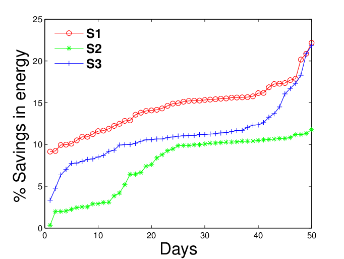
(a) Winter 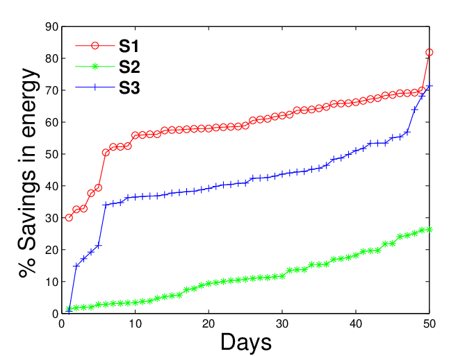
(b) Summer Figure 9: Savings in energy when using SA instead of NS for 50 different days, sorted in ascending order for the three scenarios Scenario Winter Summer 1 14.44 59.02 2 7.68 11.62 3 11.21 41.88 Table 4: Average percentage energy savings for S1, S2 and S3 We observe that in both seasons, there is a significant reduction in energy use with SA, compared to NS. In Scenario 1, this is because all the rooms have SPOT and hence there is more flexibility in the control process that uses the central HVAC only to provide a base thermal level, with SPOT providing the additional thermal offset for any rooms with occupancy.
In Scenario 2, there is a room which does not have SPOT. The central HVAC system is solely responsible for the thermal comfort in that room. Hence the occupancy pattern in the common room is the primary determinant of the HVAC system operation: if this room is occupied, the central HVAC needs to heat or cool all five rooms whether or not they are occupied. As a result, we could not obtain the same savings in energy as with Scenario 1.
In comparison to Scenario 2, we observe additional savings in energy in Scenario 3 because of the separation of the rooms with SPOT and the rooms without SPOT into separate zones. Specifically, since all rooms in one of the zones have SPOT, there is more flexibility in the VAV control for this zone. Nevertheless, the AHU control is common to both zones, so we do not obtain the same savings in energy as in Scenario 1. This analysis suggests that to maximize energy savings, SPOT should be deployed in all rooms in one entire zone at a time, rather than piecemeal.
When comparing energy savings across seasons, we observe higher savings in energy in summer than in winter. This is because in summer SPOT cools with a fan, which needs only 30 W of power, whereas in winter the SPOT heater consumes 700 W. Hence, in winter if all the rooms were occupied, it is better to employ the central HVAC to provide the appropriate thermal level as opposed to operating the HVAC at a base level along with the SPOT systems in all the rooms being ON. In other words, SPOT in heating mode is beneficial only during times of partial occupancy. In contrast, in summer, even if all the rooms with SPOT were occupied, the rooms could be at a higher temperature than the desired level with the fan in all the rooms being ON, to maintain an appropriate comfort level.
One of the significant reason for energy savings we obtain for SA is the reduced supply air temperature of the HVAC system in comparison with NS. This is illustrated in the next section.
5.2.2 AHU Supply Air Temperature
We expect that in Scenario 1, since all the rooms have SPOT, the supply air temperature could be lower (resp. higher) in winter (resp. summer) with SA than NS. This is because SPOT would supply the additional offset in comfort. Figure 10 illustrates this for a single typical day in winter and Figure 11 for a typical day in summer.

(a) Scenario 1 
(b) Scenario 2 
(c) Scenario 3 Figure 10: Comparison of supply air temperature of SA and NS for one typical winter day. 
(a) Scenario 1 
(b) Scenario 2 
(c) Scenario 3 Figure 11: Comparison of supply air temperature of SA and NS for one typical summer day. We find that, as expected, the supply air temperature with SA is lower than with NS in winter, and higher in summer. We find that the greatest differences in supply air temperature are with a full deployment of SPOT (S1), but there is a significant impact even with partial deployments (S2 and S3).
5.3 Heterogeneous Comfort Requirements
To study the case of heterogeneous comfort requirements, for simplicity, we focus on Scenario 1, that is, a building with a single zone. We assume that there are diverse comfort requirements across the rooms in this zone. These values, given in Table 7, are chosen close to the standard (ASHRAE) comfort requirements. Each user has comfort requirements that vary within a range of C.
With heterogeneous comfort requirements in a single zone, some users are likely to experience discomfort when using NS. We employ the following metric to compute overall occupant discomfort. Since the smallest time-scale of control is 30 seconds, we consider every 30s interval in a day and check if a user experienced discomfort, i.e., the PMV level in the room lies outside the range specified by the user. We define
The average saving in energy consumed and the average comfort improvement when using SA instead of NS over 25 days are reported in Table 5. Figure 12a and Figure 12b show the per-day results for winter while Figure 13a and Figure 13b show the per-day results for summer.
Table 5: Average (over 25 days) energy savings and improved comfort for the case with heterogeneous comfort requirements Season % savings in energy % improvement in comfort Winter 32 29 Summer 82 51 (a) Energy (b) Discomfort Figure 12: Percent reduction in energy when using SA instead of NS (left) and average discomfort experienced by all occupants (right) for each control scheme for 25 winter days. (a) Energy (b) Discomfort Figure 13: Percent reduction in energy when using SA instead of NS (left) and average discomfort experienced by all occupants (right) for each control scheme for 25 summer days. (a) Summer (b) Winter Figure 14: Comparing energy use and discomfort for NS and SA for different values of the weighting parameter . A quick glance at Figures 12a and 13a shows that in both seasons, SA brings a considerable reduction in energy use on most days. Moreover, Figures 12b and 13b shows that in both seasons, SA had overall lower discomfort than NS. This is because there are heterogeneous requirements in the five rooms, which could not be satisfied by the central HVAC alone.
We now comment on some interesting aspects of these figures:
- i.
- ii.
In winter there is certain amount of discomfort even when using SA. This is because, when a room becomes occupied, SPOT needs some time to heat up the space and bring the temperature to the desired level. This would result in few intervals of discomfort for the user.
- iii.
In summer, with SA, from the moment the fan is ON, the user perceives comfort and PMV reduces immediately. This process is quicker than employing the heater during Winter. Hence, with SA, with respect to comfort, we observe better performance in summer than in winter.
- iv.
With SA, we still observe a small amount of discomfort in summer. This is due to the fact that sometimes, a heater needs to be employed to satisfy some occupant’s comfort requirement (when the HVAC set point is lower than the occupant’s comfort level). During the time that it takes to heat the room, the user would experience discomfort.
Figure 14 summarizes the prior four figures and also shows the impact of the weighting value W in Equation . We see that the reduction in energy use and discomfort is greater in summer than in winter. Increasing the value of the weighting factor causes NS to expend more energy to reduce discomfort. However, even with a large expenditure in energy, NS is unable to match the performance of SA in either summer or winter, though in winter, the performance gap is smaller. Specifically, with a small value of , NS expends nearly the same energy as SA. However, this increases discomfort well beyond what is achieved by SA. Gains in comfort can only be achieved by expending more energy, even so, the comfort achieved by NS is always less than that achieved by SA.
The above evaluation shows the benefits in terms of both energy reduction and improvement in comfort of using a SPOT-aware HVAC system, as compared to a HVAC system without SPOT.
5.4 The Price of Unawareness
Ideally, a central HVAC control system should be modified to take into account the deployment of SPOT instances in the building as proposed in this paper. However, we realize that, at least at the outset, this may not always be feasible. Hence, we now evaluate another control variant, dubbed SU, where SPOT is introduced in the same rooms as in SA, but the central HVAC is unaware of the presence of SPOT, and hence chooses the same AHU and VAV set points as NS.
In the interests of space, we summarize the results for the SU scheme for Scenario 1 (full deployment of SPOT but with partial occupancy) for heterogeneous comfort requirements in Figure 15.
(a) Summer (b) Winter Figure 15: Comparing energy use and discomfort for SA, NS and SU systems for different values of the weighting parameter W. Note that SU does almost always much better than NS. The comparison of SA and SU is a little bit more challenging. In summer, the discomfort achieved by SU is statistically identical to that of SA, which is not surprising, since they both have SPOT systems. However, the energy expenditure with SU is significantly greater than that of SA.
In winter, as increases, the energy use of both NS and SU increases and their discomfort reduces, as expected. However, the discomfort of the NS system is significantly greater than with the SU and SA systems. The discomfort achieved by the SU system is lower than with the SA system for large values of (though this is not statistically significant). However, this comes at the cost of increased energy use, compared to SA. Essentially, this means that the SU controller makes a different energy-comfort trade off than the SA controller.
6 Related Work
A survey of personal comfort systems, quantifying their ability to provide comfort, can be found in [16]. In [17] a personal comfort system for cooling, essentially a fan working independent of the central cooling system, is proposed. Three versions of the SPOT system are discussed in [2, 3, 4]. The first one uses many sensors and reactive control, the second proposes MPC-based optimal proactive control, the last one uses a simple reactive control, and provides both heating (with a heating coil) and cooling (with a fan). All three are designed to work independent of the central HVAC system.
The thermal model of a room is inherently bi-linear in nature [7]. A typical approach is to linearize the model about an operating point of the supply air temperature and then develop an optimal controller using methods such as Linear Quadratic Control (LQR) theory, or fuzzy logic. [18, 19]. Since the linearization is done about an operating point, performance suffers when the operating point differs from the linearization set point. Consequently, we use a non-linear model, which avoids this problem.
For a non-linear model of the HVAC system with quadratic cost functions, feedback controllers are developed in [20]. In [21], the control of a Variable Air Volume (VAV) unit of an HVAC system is formulated as a non-linear optimization problem and solved using non-linear programming techniques. In both papers, the optimization approach is myopic.
Two comprehensive reviews of the role of MPC in HVAC systems can be found in [11, 22]. We discuss only a few relevant papers here. [23] uses an MPC for minimizing the total and peak energy consumption of HVAC systems in buildings. In [5], a hybrid system model is assumed for the HVAC system. The hybrid system is assumed to have certain number of modes, with each mode having a fixed supply temperature, and the model is assumed to be linear in each mode. A new form of MPC called Learning Based MPC (LBMPC) is used. In [6], a bi-linear system model is used and an MPC is employed. Here the operation of the HVAC system is modeled with a single time-scale. In [24] MPC-based control algorithms with special focus on occupancy information are proposed. An analysis of the local optima for non-linear MPC for a single instance of the problem is done in [7], where the influence of prediction horizon and discretization process on the local optima are investigated. Based on existing data from occupant feedback, a dynamic thermal comfort model was developed and used along with an MPC-based controller in [25]. In [26], non-linear MPC is used to determine the set points of an HVAC system, which are then implemented using PID controllers. In [27], MPC-based control strategies are adopted to individually optimize thermal comfort and energy savings. Reference [28] is a preliminary paper where we investigate the idea of two time-scale HVAC control.
In this paper, we propose a novel approach to control a centralized HVAC system that is aware of comfort requirements being met by the SPOT personal thermal comfort system. We demonstrate that our approach results in significant savings in energy in addition to providing personalized comfort. To our knowledge, no prior work has considered the control of a centralized HVAC system in the presence of such personal thermal comfort systems.
7 Conclusion
Our work addresses two intrinsic problems of modern HVAC systems, namely, coping with diverse comfort requirements, and efficiently heating or cooling partially occupied zones. We believe that using personal thermal comfort systems, such as personal heaters or fans [2, 3, 4], allows us to effectively bridge the comfort gap between what is provided by a central HVAC system and the personal preferences of the occupants. Thus, we present the detailed design an MPC-based controller for a centralized HVAC system that is aware of the deployment of personal comfort systems and uses this knowledge to exploit their responsiveness and flexibility for fine-grained thermal control.
Our control algorithm explicitly models non-linearities in the physical system, resulting in a non-linear optimization problem. It also explicitly models the physical constraints that limit the time-scales with which elements of the central HVAC system can make changes to their set points, resulting in a two time-scale MPC control.
We conduct a detailed numerical evaluation of our approach using realistic occupancy models, both in winter and in summer, and with partial and full deployment of personal comfort systems, along the twin axes of energy consumption and comfort. We find that that our system obtains, on average, 45% savings in energy in summer, and 15% in winter, compared with a state-of-the-art MPC controller, for the case when we assume homogeneous comfort requirements. For heterogeneous comfort requirements, we observe about 30% improvement in comfort in winter and about 50% in summer in addition to significant savings in energy. This validates our claims about the effectiveness of our approach.
References
References
- Underwood [2002] C. P. Underwood, HVAC control systems: Modelling, analysis and design, Routledge, 2002.
- Gao and Keshav [2013a] P. X. Gao, S. Keshav, SPOT: a smart personalized office thermal control system, Proceedings of ACM International Conference on Future Energy Systems (2013a) 237–246.
- Gao and Keshav [2013b] P. X. Gao, S. Keshav, Optimal personal comfort management using SPOT+, Proceedings of the 5th ACM Workshop on Embedded Systems For Energy-Efficient Buildings (2013b) 1–8.
- Rabbani and Keshav [2016] A. Rabbani, S. Keshav, The spot* personal thermal comfort system, Proceedings of ACM BuildSys (2016).
- Aswani et al. [2012] A. Aswani, N. Master, J. Taneja, A. Krioukov, D. Culler, C. Tomlin, Energy-efficient building HVAC control using hybrid system LBMPC, IFAC Proceedings Volumes 45 (2012) 496–501.
- Kelman and Borrelli [2011] A. Kelman, F. Borrelli, Bilinear model predictive control of a hvac system using sequential quadratic programming, IFAC World Congress (2011).
- Kelman et al. [2013] A. Kelman, Y. Ma, F. Borrelli, Analysis of local optima in predictive control for energy efficient buildings, Journal of Building Performance Simulation 6 (2013) 236–255.
- Fanger [1970] P. O. Fanger, Thermal comfort. analysis and applications in environmental engineering., Danish Technical Press, Copenhagen, Denmark (1970).
- Tyler et al. [2013] H. Tyler, S. Stefano, P. Alberto, M. Dustin, S. Kyle, CBE Thermal Comfort Tool for ASHRAE-55, Center for the Built Environment, University of California Berkeley, http://cbe.berkeley.edu/comforttool/ (2013).
- Biegler [1998] L. Biegler, Advances in nonlinear programming concepts for process control, Journal of Process Control 8 (1998) 301–311.
- Afram and Janabi-Sharifi [2014] A. Afram, F. Janabi-Sharifi, Theory and applications of hvac control systems–a review of model predictive control (mpc), Building and Environment 72 (2014) 343–355.
- ocp [????] https://github.com/rachelkalpana/occupancy-data-.
- tem [????] http://weather.uwaterloo.ca/.
- Jain [2017] M. Jain, ThermalSim: A Thermal Simulator for Error Analysis, ArXiv e-prints (2017).
- Hong et al. [2000] T. Hong, S. Chou, T. Bong, Building simulation: an overview of developments and information sources, Building and environment 35 (2000) 347–361.
- Zhang et al. [2015] H. Zhang, E. Arens, Y. Zhai, A review of the corrective power of personal comfort systems in non-neutral ambient environments, Building and Environment 91 (2015) 15–41.
- Atthajariyakul and Lertsatittanakorn [2008] S. Atthajariyakul, C. Lertsatittanakorn, Small fan assisted air conditioner for thermal comfort and energy saving in Thailand, Energy Conversion and Management (2008) 2499–2504.
- Maasoumy [2014] M. Maasoumy, Modeling and optimal control algorithm design for HVAC systems in energy efficient buildings, Master’s thesis, EECS Dept., Univ of California, Berkley (2014).
- Rahmati et al. [2003] A. Rahmati, F. Rashidi, M. Rashidi, A hybrid fuzzy logic and PID controller for control of nonlinear HVAC systems, IEEE International Conference on Systems, Man and Cybernetics, (2003) 2249–2254.
- Arguello-Serrano and Vélez-Reyes [1999] B. Arguello-Serrano, M. Vélez-Reyes, Nonlinear control of a heating, ventilating, and air conditioning system with thermal load estimation, IEEE Transactions on Control Systems Technology 7 (1999) 56–63.
- Zheng and Zaheer-Uddin [1996] G. Zheng, M. Zaheer-Uddin, Optimization of thermal processes in a variable air volume hvac system, Energy 21 (1996) 407–420.
- Kwadzogah et al. [2013] R. Kwadzogah, M. Zhou, S. Li, Model predictive control for HVAC systems - a review, IEEE International Conference on Automation Science and Engineering (CASE) (2013) 442–447.
- Maasoumy and Sangiovanni-Vincentelli [2012] M. Maasoumy, A. Sangiovanni-Vincentelli, Total and peak energy consumption minimization of building HVAC systems using model predictive control, IEEE Design & Test of Computers 29 (2012).
- Goyal et al. [2013] S. Goyal, H. A. Ingley, P. Barooah, Occupancy-based zone-climate control for energy-efficient buildings: complexity vs. performance, Applied Energy 106 (2013) 209–221.
- Chen et al. [2016] X. Chen, Q. Wang, J. Srebric, Occupant feedback based model predictive control for thermal comfort and energy optimization: A chamber experimental evaluation, Applied Energy 164 (2016) 341–351.
- Castilla et al. [2014] M. Castilla, J. Álvarez, J. Normey-Rico, F. Rodríguez, Thermal comfort control using a non-linear mpc strategy: A real case of study in a bioclimatic building, Journal of Process Control 24 (2014) 703–713.
- Freire et al. [2008] R. Z. Freire, G. H. Oliveira, N. Mendes, Predictive controllers for thermal comfort optimization and energy savings, Energy and buildings 40 (2008) 1353–1365.
- Kalaimani et al. [2016] R. K. Kalaimani, S. Keshav, C. Rosenberg, Multiple time-scale model predictive control for thermal comfort in buildings, Proceedings of the Seventh International Conference on Future Energy Systems Poster Sessions (2016) 11.
Appendix
In this section we list the numerical values of various parameters of our model that was used in our analysis. The optimization problem is also tabulated.
Table 7: Parameter Values (Set of zones) (Set of rooms of Type in zone ) (Set of rooms of Type in zone ) Given : Measured parameters at time : Outside temperature and room occupancy , , , Room temperature in region 1 and 2, , , . System parameters: , , , , , , , ¯ u ,_i, ¯ v _i, ¯ V _a,∀i∈I θ 1 ,θ 2 ,θ 3 ,θ 4 ,θ 5 ,f 1 ,f 2 ,f 3 ,f 4 . Comfortparameters: ¯ γ , ¯ γ , ¯ κ , ¯ κ , ¯ β i j , ¯ β i j ,∀j∈R i 1 ∪R i 2 ,∀i∈I. Inputvaluesfrompreviousstep(tobeusedifq≠0): U Objective: { u ( k ) , v ( k ) , r ( k ) , w i j ( k ) , v a i j ( k ) , T m ( k ) , T c ( k ) , x 1 i j ( k ) , x 2 i j ( k ) , P i j ( k ) } Minimize ∑ k = T J(k)τ, whereJ(k):= i ∈ I ∑ v i (k)θ 1 (u(k)-T c (k))+ i ∈ I ∑ v i (k)θ 2 (T m (k)-T c (k))+θ 3 ( i ∈ I ∑ v i (k)) 2 +θ 4 i ∈ I , j ∈ R i 1 i ∑ w i j (k)+θ 5 i ∈ I , j ∈ R i 1 i ∑ v a i j (k). Constraints: x i j (k+1)=A 0 i (i,i)x i j (k)+A 1 i (i,i)x i j (k)v i (k)+B i (i)u(k)v i (k)+D 1 i (i,i)(k)T o (k) +D 2 i (i)(k)O i (k),∀j∈R i 1 ∪R i 2 ,∀i∈I,∀k∈T. Δx i j (k+1)= ~ A 0 i (i,i)Δx i j (k)+ ~ B i (i)w i j (k),∀j∈R i 1 ,∀i∈I,∀k∈T. x 1 i j (k+1)=x i j (k+1)+Δx i j (k+1),∀j∈R i 1 ,∀i∈I,∀k∈T. x 2 i j (k+1)=x i j (k+1)+D 3 Δx i j (k),∀j∈R i 1 ,∀i∈I,∀k∈T. T m (k)=[r(k) 1 m n i ∈ I , j ∈ R i 1 ∪ R i 2 ∑ x i j (k)]+(1-r(k))T o (k),∀k∈T. P i j (k+1)=f 1 x i j (k+1)+f 2 v a i j 2 (k)+f 3 v a i j (k)+f 4 ,∀j∈R i 1 ,∀i∈I,∀k∈T. ¯ β i j ≤P i j (k)≤ ¯ β i j ,O i j =1,∀i∈I,j∈R i 1 ,∀k∈T. ¯ γ ≤x 1 i j (k)≤ ¯ γ ,O i j =1,∀i∈I,j∈R i 1 ,∀k∈T ¯ κ ≤x i j (k)≤ ¯ κ ,O i j =1,∀i∈I,j∈R i 2 ,∀k∈T. ¯ γ ≤x i j (k)≤ ¯ γ ,∀i∈I,j∈R i 1 ∪R i 2 ,∀k∈T. 0≤w i j (k)≤1∀j∈R i 1 ∀i∈I,∀k∈T. 0≤v a i j (k)≤ ¯ V a ∀j∈R i 1 ∀i∈I,∀k∈T. w i j (k)≤O i j (k)∀j∈R i 1 ∀i∈I,∀k∈T. v a i j (k)≤O i j (k) ¯ V a ∀j∈R i 1 ∀i∈I,∀k∈T. r(k)≤0.8,∀k∈T. T c (k)≤T m (k),∀k∈T. u(k)≥T c (k),∀k∈T. ¯ u ≤u(k)≤ ¯ u ,∀k∈T. ¯ v ≤ i ∈ I ∑ v i (k)≤ ¯ v ,∀k∈T. Ifq=0,u(6z+ℓ)=u(6z+j+ℓ),z∈{0,1,2,3},j∈{1,..,5}. Ifq≠0,u(ℓ)=U, u(ℓ)=u(ℓ+j),j∈{0,1,..,5-q}, u(ℓ+6z-q)=u(ℓ+6z-q+j),z∈{1,2,3},j∈{1,..,5}. u(ℓ+6z-q)=u(ℓ+6z-q+j),z=4,j∈{0,1,..,q-1}. ThematricesinthethermalmodelareexplainedinSection3.1and3.2.Thevaluesofθ_1θ_2ρ,σ,η_hη_cf_i
- (a)
