Thermal Source Localization Through Infinite-Dimensional Compressed Sensing
E-mail: flinth,hashemi@math.tu-berlin.de
August 24, 2026
Abstract
We propose a scheme utilizing ideas from infinite dimensional compressed sensing for thermal source localization. Using the soft recovery framework of one of the authors, we provide rigorous theoretical guarantees for the recovery performance. In particular, we extend the framework in order to also include noisy measurements. Further, we conduct numerical experiments, showing that our proposed method has strong performance, in a wide range of settings. These include scenarios with few sensors, off-grid source positioning and high noise levels, both in one and two dimensions.
1 Introduction
Monitoring temperature over spatial domains is an important task with practical importance for surveillance and automation purposes [19]. Areas of application include agriculture [1], climate change studies [39], thermal monitoring of CPUs [33], and environmental protection [37]. Other applications include monitoring of the thermal field caused by on-chip sensors for many-core systems [33, 29], and cultivation of sensitive species [16]. For these and similar applications, it is necessary to monitor the temperature with high resolution using a proper sampling device for possibly long term periods. One possible way to do this is to estimate the positions of the initial heat sources.
1.1 Previous Works and Literature Review
Solving the inverse problems involving the heat or diffusion equation has a reach history coming back to estimate the initial temperature of the earth by Fourier and Kelvin [32]. These inverse problems and strategies to solve them efficiently has attracted much attention recently, due to the numerous challenges that we are facing in real-world applications. First of all, we usually have a tight constraint on the number of sensors in practice, e.g. due to economical constraints. These sensors also usually have limited power supply as well. There is no need to mention that, the nature is not always cooperating with us; therefore, we have noise and interference issues. These factors make the heat involving inverse problem hard to solve. Hence, we need to somehow incorporate inherent structure of thermal field as a side information and utilize an intelligent machinery in order to tackle this tricky problem.
In the literature, many strategies for attacking the problem of thermal field and/or source estimation can be found. Let us summarize a few of the more recent ones.
Regarding the mathematical analysis, the authors in [7, 31] provide fundamental error bounds on the aliasing error of reconstructing a diffusion field. The main argument is that the diffusion process inherently acts as a low pass filter. Hence, although the spatial bandwidth of the diffusion field is infinite, it can still be well approximated by a signal with low bandwidth. Considering this fact the authors proposed a method for reconstructing the thermal field generated by initial sources. This contribution is extended in [30] for addressing the problem of time-varying sources by considering time varying emissions rates lying in two specific low dimensional sub-spaces.
This effort has been extended by Murray et al. [23, 22], exploiting Prony’s method for localized sources in order to estimate the locations in space and time of multiple sources. In a very recent work, they extended their method to distributed sensor networks [24],and to non-localized sources of diffusion fields, in particular to straight line and polygonal sources [25], respectively. They furthermore consider other governing equations, such as the wave and Poisson equations [26]. However, these works assume a relatively large amount of field samples to be accessible, which may not be possible in a wide range of applications.
The works mentioned above do not address the problem of reducing the number of spatiotemporal samples in an efficient way. This is instead done in [33, 29], where the problem of low resolution in thermal monitoring of a CPU is considered. Their proposed method consists in selecting the most informative sensors utilizing a frame potential objective function based on the Unit-Norm-Tight-Frame (UNTF) concept. Although the paper emphasizes on empirical aspects, theoretical claims are also derived.
Excluding [23, 22], all of the previously mentioned works do not explicitly try to utilize the useful structures which exist for diffusion sources, such as sparsity and spatiotemporal correlation among measurement governed by a PDE constraint. In particular, none of them use the powerful framework of compressed sensing [2]. Therefore, Rostami et al. [34] proposed a compressed sensing method for reconstructing the diffusion field by incorporating PDE constraints in recovery part as a side information. This effort was extended to the 2D scenario in [15] by one of the authors of this article, together with co-authors. In a similar way but by utilizing an analysis formulation for the source localization problem, [17] consider the source localization inverse problem for other types of sources or governing equations, with PDE side information in a co-sparse framework.
1.2 Contributions
The contribution of this work is threefold: As we have seen in the preceding section, rigorous theoretical guarantees for the methods described above are relatively scarce. Therefore, our first contribution in this paper is to provide mathematical guarantees and proofs rigorously showing that our recovery framework will provide solutions which, in a certain sense, are close to the ground truth solutions. This type of recovery, coined soft recovery, was recently developed by one of the authors in [10]. In this paper, we in fact extend the theoretical soft recovery framework to a setting with noisy measurements – a mathematical contribution important on its own.
Secondly, the subtle problem of off-grid source positioning has not been considered so far in the thermal source localization literature, to the best knowledge of the authors. The proposed schemes in the area assume a fixed grid, on which a discretized version of the continuous field is defined. A fixed grid does not only cause discretization errors, but it also has problems capturing sources which have positions between the grid points [6]. In this work, we address this issue by employing the philosophy of [35, 3, 9]. That is, we consider the recovery problem in a continuous domain. This approach automatically tackles the discretization error and off-grid challenge, since it in some sense uses an infinite dimensional grid.
The final contribution of this paper consists in its robustness toward the insufficient number of spatiotemporal measurements and also ill-conditioning of the Green function matrix. While most proposed methods in the literature assume a large number of accessible measurements, the numerical results based on the idea proposed in this paper demonstrate a very satisfactory performance, already when we only have access to one time sample and a very small subset of spatial samples. These results could have a significant impact on applications which have a tight constraint on the number of spatiotemporal samples due to financial costs, energy consumption, physical limitation or other application specific issues. Besides, the recovery procedure is much more robust to the ill-conditioning of the system model matrix consisting of Green functions compared to the classical results in the literature. In Section 3, we validate the robustness of our method numerically.
2 Problem Formulation and Theoretical Analysis
2.1 Problem Formulation
The governing equation for propagation of heat is the heat equation. Its most rudamentary form is as follows
| (1) |
Here is the Laplace operator and is the initial heat distribution. In this work, we will model it as a linear combination of finitely many point sources:
| (2) |
where , and denote the number of sources, their amplitudes and locations, respectively. Note that although this model is quite idealized, it is commonly used in the literature (often under the name of instantaneous sources). We choose to denote the ground truth distribution by , since it is a measure. We will for convenience make the global normalization assumption
It is well known that (1) has a unique solution for initial values of the type (2) – and even that the solution is given by convolution of with the Green function , i.e.
| (3) |
As was already mentioned, is a measure. More specifically, is a member of the space of (signed) Radon measures of finite variation. That space is naturally equipped with the total variation norm:
The -norm can intuitively be viewed as the infinite-dimensional analogue of the -norm of a vector in . This becomes especially clear when considering that the norm of a train of -peaks (2) is equal to . Knowing that -minimization promotes sparsity, it seems reasonable to minimize the -norm to recover a signal like (2) from linear measurements :
| () |
is thereby given through samples of the function (3), expressed by the linear measurement operator . This idea is per se not new (see for instance [35, 3, 9]), but we believe that it is the first time that this method is proposed for solving the source localization problem.
2.2 Theoretical Analysis
Very generally, the solution of a problem of the type (and also of the type defined below) has a structure of the form
where is the dimension of the measurement vector (see [11, 38]). In this paper, we will use the theory from [10, Sec. 4.3] to theoretically guarantee that the positions of the sources in the reconstructed signal are at least close to the positions of the ground truth sources. Thereby, we in some sense circumnavigate the fact that the dictionary (i.e. the operator ) is highly coherent. In fact, we will even extend the soft recovery framework to also include noisy measurements.
We start by quickly reviewing the mentioned theory (we leave out a lot of technical details for now – they are instead discussed in the appendix 5.2 ). Let be an -normalized low-pass filter: To be concrete, let us say for some . Define the Hilbert space as the space of tempered distributions having the property , with scalar product
| (4) |
is then a normalized dictionary in , since . In particular, our ground truth measure (2) is a member of . Let us furthermore associate an autocorrelation function to the filter through
We are now ready to cite the result we wish to apply.
Theorem 2.1.
[10, Cor. 4.3] Let , , , and be as above, (for some ) be a continuous linear operator, and be arbitrary. If there exists a , where denotes the Fourier transform, with
| (5) |
where are parameters, then for every solution of , there exists an with
| (6) |
Remark 2.2.
Note that for our function , a bound of the form (6) immediately implies a bound on the proximity of to :
In practice, measurements are always contaminated with noise – that is, we do not have access to , but rather a noisy version , with . A canonical extension of to handle this setting is to consider the following ”” (the term is from [36], where it was coined in a finite-dimensional setting):
| () |
where . In the appendix, we will extend the soft recovery framework to include also such problems. For the –problem, we obtain the following result.
Corollary 2.3.
Remark 2.4.
The previous theorems only secure that each peak in the ground truth measure can be approximately retrieved in the solution (i.e. softly recovered). This is of course important on its own, but let us also note that an approximate recovery of the peaks is enough to secure good reconstruction of the temperature field ! If and are close, the corresponding active dictionary elements and also are, so interchanging them in the decomposition does not have much of an effect.
In [10], the case that the measurement operator consists of sampling the coefficients of the signal in a so-called frame of is discussed. A frame is thereby a family of vectors in a Hilbert space obeying the frame inequality
for some scalars (frame bounds) .
In this work, our measurements are of an entirely different nature: namely samples of the solution, (3), of the heat equation. If we call the sample set , the measurement operator is hence given by
| (7) |
Note that is defined on the whole of , since we can convolve the Green function with any tempered distribution, in particular elements of . is, provided , furthermore continuous as an operator on , which the following lemma shows. Its proof can be found in Section 5.1.1 of the Appendix.
Lemma 2.5.
If for all , is a continuous operator from to , with . Its adjoint is given by
where is defined as .
Lemma 2.5, Theorem 2.1 and Remark 2.2 tell us that if we can construct a function of the form
| (8) |
which satisfies (5), we are done (note that ). The rest of the section will be devoted to this cause.
The strategy will be the following: If we could choose as , we would immediately have (5) for and (remember that we assumed that for all , and that is a positive function). is however not always of the form (8) – the Gaussians in (8) neither have the same width nor the same centers as the Gaussian . The former problem can be solved by assuming for – note that can per se be freely chosen, so this equality is always achievable. The latter problem is then to approximate a Gaussian of width centered at with other Gaussians of width centered at the points on the grid. In order to be able to give a concrete proof that this is possible, let us make the following assumptions:
- •
is located in the rectangle .
- •
The samples are all taken at time and spatially on a uniform grid over with spacing for some , i.e.
(9)
Given this structure of the samples, the mathematical task at hand is to do the following: Denoting our Gaussian with , we need to approximate with a linear combination of the functions , . By translating everything and possibly discarding some of ’s, we can bring this down to approximating with functions , and :
| (10) |
The approximate equality is thereby supposed to be true uniformly in . Since
| (11) | ||||
the problem boils down to the question: How well can we approximate the function with sums of complex exponentials with ? (Note that we from the second line and forward left out the range of summation for in order to not overload the notation. We will continue doing this in the sequel.)

This question can be solved with routine techniques – a detailed proof is given in the appendix. One arrives at the following statement.
Lemma 2.6.
There exists scalars with
The vector obeys .
A full proof of Lemma 2.6 can be found in Section 5.1.2 of the appendix. Here, we will instead state and prove the main theoretical result of this paper.
Theorem 2.7 (Main Result).
Let and suppose that the sample set has the structure (9) with . Then if then for every minimizer of , there exists a with .
In fact, also in the case that with , the regularized problem for every has the following property: For every minimizer of , there exists a with . Put shortly, the bound for the noiseless case deteriorates gracefully with a non-optimal choice of and increasing noise level.
Proof.
Lemma 2.6 together with the structure of and the form of (see Lemma 2.5) implies that for any , there exists a with
This satisfies, for a constant ,
where we used that both the coefficients as well as the function are positive when discarding all terms but the one related to in the second step. In the last step, we inferred the normalization assumption on . We furthermore have
Hence, if we choose , (5) is satisfied for
Now Theorem 2.1 implies that any minimizer of possesses a point in its support with
if we choose . This implies .
As for the noisy case, Corollary 2.3 implies that any minimizer of possesses a point in its support with
We used that . Now, the first one of these terms were estimated to be larger than in the argument for the non-noizy case. As for the second, we have:
since . This, together with the estimate on , implies
which yields
∎
Remark 2.8.
As is common in the compressed sensing literature, the theorem provides a lower bound on the amount of measurements needed to secure approximate recovery of the source positions. The bound grows with decreasing and amplitude . This is sound: The lower the , the higher is the precision, and the smaller , the less significant is the peak.
Note that if all peaks are equally large, exactly equals the sparsity of the signal (remember that we assumed .) hence corresponds to , which unfortunately is suboptimal. (A linear dependence on the sparsity is asymptotically optimal – even if we are a priori given the positions , we will still need measurements to determine the amplitudes .) This may well be an artefact of the proof, since it solely relies on approximation properties of the Fourier basis (which is well known to struggle in high dimensions). We leave the question whether an improvement is possible as an open problem.
Reducing the number practically corresponds to lowering the number of spatiotemporal samples. This will reduce the financial cost. Also, it will enable satisfactory reconstruction results in applications where there are very tight constraints on the number of sensors or time samples.
This concludes our theoretical analysis, and we move on to test our method numerically.
3 Numerical Experiments
In this section, we numerically demonstrate that our proposed method performs well in practice. To start, we work in a one-dimensional regime. The main reason for this is to be able to make a comparison with the method proposed in [28], which to the best knowledge of the authors is the state-of-the art compressed-sensing based method for recovery of sparse initial source distribution in thermal source localization. Note that there are more recent methods for thermal field reconstruction, as was explored in the introduction. These can however not be fairly compared to our method. The method the authors of [17, 18] mainly advertise uses a different type of sparsity than we do. In their setting, is sparse in a certain sense, where is an analysis operator. This is completely different from our sparsity, which is in the direct sense for the initial condition. On the other hand, the works [23, 26] assume a model in which the sparse recovery problem can be reformulated as the problem of recovering a sum of sinusoids with unknown frequencies, where the Prony method is applicable. This is not immediate in our setting.
Although the theory developed previously applies to the 2D-case, we will first stay in a 1D-regime here. The reason for this is twofold: First, [28] only consider the 1D-case, so only in this regime, a fair comparison can be made. By doing extensive numerical experiments on synthetic data, we compare the performance of the method from [28] and the one proposed in this work, in several cases. In particular, we consider scenarios with noisy measurements, sources off-the-grid, and also cases where the number of samples is too small for the method [28] to work.
In the second part of this section, we will present the results also for 2D case. Let us begin by describing the method in [28].
3.1 Brief Review of the Structure of the Simulation and Comparing Method
The authors in [28] introduced a sampling procedure for fully reconstructing the unknown initial field distribution from spatiotemporal samples collected at time from a diffusion field which is generated by sources. By constructing a sensing matrix through discretizing the diffusion field, and reformulating this matrix as a function of spatial and temporal sampling densities, they derive precise bounds for spatial and temporal densities under which the sensing matrix is well-conditioned for solving this inverse problem.
For introducing the initial inverse problem in discrete form similar to [28], we assume that the sources are deployed on a grid of size , with some separation. Then, we define for representing the spatial location of these sources as follows:
| (12) |
where . We hence assume that the diffusion field propagates in one dimension with length . Also, we define a vector representing the amplitude of the source. Concretely, the amplitude at -th position of the grid is given by
We will assume that is -sparse, with , similar to [28]. Note that this is a slight simplification compared to (2), where the sources are not confined to lie on the grid.
For sensing the diffusive field in this scenario, we consider a sensor network with spatial sensors deployed uniformly in , each one collecting uniform time samples. Hence, we have a spatiotemporal sampling procedure which provides us samples and we aim to estimate the initial source parameters, and , using these samples.
Similar to [28], we also define and for representing the spatial position of sensors and temporal sampling grid, respectively:
where is the distance between spatial sensors in spatial domain. denotes the time interval between two time samples. Then, the vector is obtained by concatenating all the samples collected by all the sensors, aiming to find a sensing matrix with size for relating and as a discrete linear equation as follows:
| (13) |
The matrix is constructed by using a discrete version of the Green function, assuming the diffusion parameter without loss of generality, and the position of sensors to be , :
| (14) |
Equation (14) describes the elements of the sub-matrix which results when sampling the field by collecting all spatial samples at one time instant, . The following equation is then a discretized version of the inverse problem considered in this publication:
| (15) |
where is the vector collected all spatial samples at the sampling instant . Finally, the matrix is constructed by concatenating sub-matrices into one matrix. Accordingly we define a vector by concatenating the vectors , each one containing all spatial samples at each sampling time [28].
Finally, by introducing a parameter , [28] proposed the following bounds on :
| (16) |
These bounds imply that the system model matrix suitable for solving the target inverse problem. [28].
3.2 Description of our Method
Now we describe how numerically implement our proposed method. A diffusive field, generated by initial sources is considered. As mentioned in the previous section, we do not assume a fixed grid for deploying the sources. Therefore, the measurements are directly captured using the closed form solution of the Green function. Using Equation (3), we see that the following equation can be used to collect the samples:
| (17) |
where the samples are taken by evaluating (17) on some set of sampling points . We can, and will, choose , but other choices are certainly possible.
The values of the source positions, , are also assigned in a grid-less manner based on on/off-grid settings which we will consider in our simulation scenario. The captured spatiotemporal samples are then concatenated to form the vector . For demonstrating the robustness of algorithm against insufficiently many samples, as well as staying as close as possible to the theoretical setting, we sense the field at only one time instant. Therefore, we only access to one time sample for the whole sensing procedure.
After obtaining the measurement vector , our goal is to solve either , or (depending on whether the measurements are noisy or not). This is in general hard. There are a few special cases in which the problem can be reduced to a finite-dimensional problem – most notably in the case of Fourier measurements [3, 8]. (See also [11] for a few more examples.) In this setting, however, such a reduction seems very hard, whence we instead propose the following (heuristic) scheme11 1 Developing a theory for such a discretization is an interesting line of research for future work. Some initial results concerning discretizations of this kind can be found in [9].: We initially restrict our analysis to a rough grid, (as in (12), but with small). We then solve the dual problem of the coursely discretized problem. For the infinite-dimensional dual problem, the points where the dual certificate has modulus one exactly corresponds to the positions of the peaks in the solution of [9]. Thus, by observing where the value of the dual certificate (where is the solution of is larger than a threshold close to (Figure 2), we get a rough idea where the peaks of the infinite-dimensional solution are located.
For the non-regularized problem , the dual of the discretized problem has a simple structure:
| () |
This is no longer the case for the problem [27]. Therefore, we deviate a bit from the theory presented above and instead, as is usual, consider the following, unconstrained version of the LASSO:
| () |
It is well known that for each parameter , there is a such that the solution of is equal to the one of [12, Theorem B.28, p.562]. Considering the fact that the parameter (or , respectively) anyhow needs to be fine-tuned, making this transition is justified. The dual problem of again has a simple form:
| () |
In next step, we refine the resolution of our dictionary by adding extra points close to the selected points from the previous step, re-discretize, and solve the corresponding dual problem (see Figure 2). We repeat the same procedure until a stopping criterion is met.
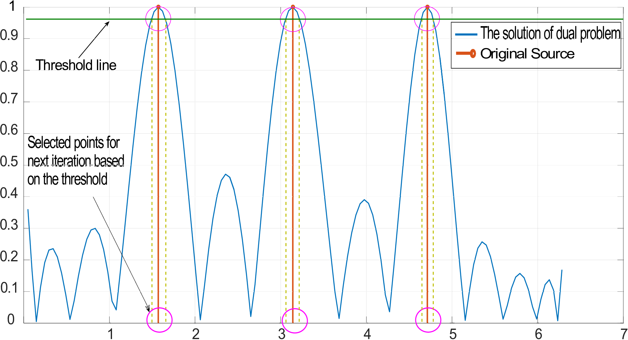
The final dual certificate is then used to obtain the estimated position of the sources. Concretely, the points with are grouped into clusters (this is easy, since we are in a -regime). For each such cluster, we choose the midpoint to be a member on the final grid .
In the final step, we build the solution by making an ansatz in the form of a sum of Dirac-’s supported on . The amplitudes of the peaks are obtained by solving the inverse problem using the pseudo inverse of the dictionary matrix constructed by the atoms corresponding to the final selected points :
where . Under the assumption that the set of chosen points contains for each ground truth peak exactly one point close to , and apart from that only points far away from all points in the ground truth support , will be close to the ground truth signal. The following formal statement holds.
Proposition 3.1.
Let be a set of ground truth peaks with the property that the matrix has full rank, and . Then for each , there exist with the following property: If with
such that
with
The arguments to obtain this result are relatively standard. For completeness, we include them in the appendix.
3.3 Simulation Results in
Now, we carry out the numerical experiments to compare the two strategies described above. In all experiments, we assume thermal sources inducing at time along with a bar with the length . The amplitudes of all sources are assumed to , for simplicity. The grid-line source distribution for comparing methods is assigned as, .
We fix the number of sensors for all experiments. Note that this is much smaller than . We furthermore only take one time sample, say at , as was done in the theoretical section. Accordingly, . The parameter is chosen as , so that it obeys the bound (16). We then perform two experiments: First, we generate data from assigning source positions on the grid. Then, we instead choose them off the grid. Then, we compare the two methods in the case that the measurements are contaminated by Gaussian noise of strength . The last experiment is also repeated for , which clearly violates the bound (16).
Note that the method from [28] assumes that the sources are on the grid, and is only guaranteed to work when obeys the bound (16)(at least in the noisy case). We still choose to test its performance for cases when these two assumptions are not met, in order to demonstrate possible improvements using our method.
As is suggested in [28], we apply the smoothed (SL0) method [21] to solve the inverse problem . For our proposed scheme, we choose the threshold for iteration , and the stopping criterion , where is the optimal value of the :th optimization problem . For the optimization, we use cvx, a package for specifying and solving convex programs [14, 13].
3.3.1 Results for Noiseless Measurements
The results for the experiments are presented in Figure 3. As can be seen, the method proposed in this paper almost perfectly recovers the peaks, both in the on-grid as well as in the off-grid case, whereas the peaks of the signal recovered by the method from [28] are ’smeared out’, making exact localization of the positions hard. This furthermore leads to the amplitudes being incorrectly recovered. Note that the performance of our method is similar in the on- and off-grid case, whereas the performance deteriorates slightly when going off-grid for the one proposed in [28]. In particular note the tendency to a spurious peak at for the latter method in the off-grid case.


The fact that our method is robust against violating the bound (16) for well-conditioning the system dictionary matrix can also provide a significant impact in scenarios where one is willing to monitor the heat induction close to the beginning of a thermal activity. In these settings, the sensing machinery including time and space densities does not have to obey any bound, and one can monitor the target activity with the desired frequency and time sampling density.
3.3.2 Results for Noisy Measurements
We now compare the performance of the introduced method in presence of noise. It should be mentioned that the noisy scenario is not addressed in [28]. This is not surprising, considering the highly ill-conditioned properties of the system model matrix, . Still, we use this method as a comparison of performance in presence of noise.
We manually tune the parameter in to for our simulation procedure, where is the variance of Gaussian white additive noise showing its power. We also set smaller stopping criteria, , in this simulation, for having more accuracy compared to the noiseless simulations.
Figure 4 demonstrate the results of the two methods in noisy settings when the signal-to-noise ratio (SNR) is equal to . As can be seen, the method proposed in [28] completely fails, both when is within, as well as without, the bounds given by (16). Note that in the case that violates (16), the outputted signal has amplitudes in a range of , suggesting that the reason for the failure is the ill-conditioning of . The method we propose, on the other hand, in both cases delivers a very sharp estimate of both the amplitudes as well as source locations as well.


3.4 Simulation
Let us finally test the performance of the method in the case of two dimensions. From a mathematical point of view, the procedure is exactly as before. From a practical point of view, we make one adjustment: Due to the increase of number of points in the grid, performing the optimization using explicit matrices and a standardized software like cvx is not feasible. Instead, we implement the primal-dual method [4], which only requires the operations and to be implemented as operators.
In order to find the points where the final dual certificate has absolute value , we used the following heuristic: First, we recorded all points in which the certificate had an absolute value larger than a certain threshold. This threshold was manually tuned to optimize the performance. These points where typically clustered around the peaks (this is due to the design of our method: close to the peaks, a lot of points are added during the iterations). Therefore, we performed a -means clustering to decide initial positions of the peaks. Using these initial positions, we then performed a gradient descent to find the local maxima of , which we finally used as our final grid .

(a)

(b)

(c)
In Figure 5, we plot the reconstructed source localizations, compared to the ground truth ones, for different noise levels. We see that the performance is good, and it gracefully tackles the noise, producing reasonable results even for low SNR regimes like .
Figure 6 demonstrates the amplitude of the reconstructed sources compared to the original ones, in a low SNR setting, .


4 Conclusion
In this paper we addressed the thermal source localization problem which has a wide range of applications and has attracted a lot of attention, recently. Based on infinite-dimensional compressed sensing theory, we proposed a method relying on TV-norm minimization for recovering the amplitudes and locations of the thermal sources in a 2D scenario. Using the soft recovery framework from [10], we provided rigorous mathematical guarantees, showing that the placements of the thermal sources will be approximately recovered by our method. In fact, we even extend the mentioned framework to include noisy measurements, which has an interest on its own
Based on the theoretical analysis, we have proposed a heuristic scheme in order to implement the infinite dimensional setting, and performed numerical simulations in a different circumstances for validating our methods. The numerical results demonstrate significantly increased performance and robustness of our proposed method compared to classical algorithms. In fact, it can tackle several challenges and phenomenons in this area such as insufficient number of spatiotemporal samples, highly ill-conditioning property of Green function matrix specially in noisy environment, discretization error and off-grid sources positioning issue.
Acknowledgements
Axel Flinth acknowledges support from the Deutsche Forschungsgemeinschaft (DFG) Grant KU 1446/18-1. He also wishes to thank Jackie Ma and Philipp Petersen for interesting discussions on this and other topics.
Ali Hashemi acknowledges support from Berlin International Graduate School in Model and Simulation based Research (BIMoS). He also would like to thank Saeid Haghighatshoar and Ngai-Man Cheung for interesting discussions on CS applications for source localization inverse problem.
Both authors also acknowledge support from the Berlin Mathematical School (BMS). They further wish to thank Gitta Kutyniok for careful proofreading and valuable suggestions for improving the paper.
References
- [1] J. Baviskar, A. Mulla, A. Baviskar, S. Ashtekar, and A. Chintawar. Real time monitoring and control system for green house based on 802.15. 4 wireless sensor network. In Communication Systems and Network Technologies (CSNT), 2014 Fourth International Conference on, pages 98–103. IEEE, 2014.
- [2] E. Candès and T. Tao. Decoding by linear programming. IEEE T. Inform. Theory, 51:4203–4215, 2005.
- [3] E. J. Candès and C. Fernandez-Granda. Towards a mathematical theory of super-resolution. Comm. Pure and Appl. Math., 67(6):906–956, 2014.
- [4] A. Chambolle and T. Pock. A first-order primal-dual algorithm for convex problems with applications to imaging. J. Math. Imag. Vis., 40(1):120–145, 2011.
- [5] V. Chandrasekaran, B. Recht, P. A. Parrilo, and A. S. Willsky. The convex geometry of linear inverse problems. Found. Comp. Math., 12(6):805–849, 2012.
- [6] Y. Chi, L. L. Scharf, A. Pezeshki, and R. A. Calderbank. Sensitivity to basis mismatch in compressed sensing. IEEE T. on Sig. Proces., 59(5):2182–2195, 2011.
- [7] I. Dokmanić, J. Ranieri, A. Chebira, and M. Vetterli. Sensor networks for diffusion fields: detection of sources in space and time. In Communication, Control, and Computing (Allerton), Annual Allerton Conference on, pages 1552–1558. IEEE, 2011.
- [8] C. Dossal, V. Duval, and C. Poon. Sampling the Fourier transform along radial lines. arXiv preprint arXiv:1612.06752, 2016.
- [9] V. Duval and G. Peyrè. Exact support recovery for sparse spikes deconvolution. Found. Comput. Math., 15(5):1315–1355, 2015. doi:10.1007/s10208-014-9228-6.
- [10] A. Flinth. Soft recovery with general atomic norms. arXiv preprint. arXiv:1705.04179, 2017.
- [11] A. Flinth and P. Weiss. Exact solutions of infinite dimensional total-variation regularized problems. In preparation, 2017.
- [12] S. Foucart and H. Rauhut. A mathematical introduction to Compressed Sensing. Birkhäuser, 2013.
- [13] M. Grant and S. Boyd. Graph implementations for nonsmooth convex programs. In V. Blondel, S. Boyd, and H. Kimura, editors, Recent Advances in Learning and Control, Lecture Notes in Control and Information Sciences, pages 95–110. Springer-Verlag Limited, 2008.
- [14] M. Grant and S. Boyd. CVX: Matlab software for disciplined convex programming, version 2.1. http://cvxr.com/cvx, Mar. 2014.
- [15] A. Hashemi, M. Rostami, and N.-M. Cheung. Efficient environmental temperature monitoring using compressed sensing. In Data Compression Conference (DCC), 2016, pages 602–602. IEEE, 2016.
- [16] J. Jiang, C. Wang, M. Liao, X. Zheng, J. Liu, C. Chuang, C. Hung, and C. Chen. A wireless sensor network-based monitoring system with dynamic convergecast tree algorithm for precision cultivation management in orchid greenhouses. Precis. Agric., pages 1–20, 2016.
- [17] S. Kitić, L. Albera, N. Bertin, and R. Gribonval. Physics-driven inverse problems made tractable with cosparse regularization. IEEE T. Sig. Proces., 64(2):335–348, 2016.
- [18] S. Kitić, S. Bensaid, L. Albera, N. Bertin, and R. Gribonval. Versatile and scalable cosparse methods for physics-driven inverse problems. In Compressed Sensing and its Applications, 2017.
- [19] H. Liu, Z. Meng, and S. Cui. A wireless sensor network prototype for environmental monitoring in greenhouses. In Wireless Communications, Networking and Mobile Computing (WiCom), International Conference on, pages 2344–2347. IEEE, 2007.
- [20] G. G. Lorentz. Approximation of Functions. Halt, Rinehart and Winston, 1966.
- [21] H. Mohimani, M. Babaie-Zadeh, and C. Jutten. A fast approach for overcomplete sparse decomposition based on smoothed -norm. IEEE T. Sig. Proces., 57(1):289–301, 2009.
- [22] J. Murray-Bruce and P. Dragotti. Spatio-temporal sampling and reconstruction of diffusion fields induced by point sources. In 2014 IEEE International Conference on Acoustics, Speech and Signal Processing (ICASSP), pages 31–35. IEEE, 2014.
- [23] J. Murray-Bruce and P. L. Dragotti. Estimating localized sources of diffusion fields using spatiotemporal sensor measurements. IEEE T. Sig. Proces., 63(12):3018–3031, 2015.
- [24] J. Murray-Bruce and P. L. Dragotti. Physics-driven quantized consensus for distributed diffusion source estimation using sensor networks. EURASIP J. Adv. Sig. Pr., 2016(1):1–22, 2016.
- [25] J. Murray-Bruce and P. L. Dragotti. Reconstructing non-point sources of diffusion fields using sensor measurements. In IEEE International Conference on Acoustics, Speech and Signal Processing (ICASSP), pages 4004–4008. IEEE, 2016.
- [26] J. Murray-Bruce and P. L. Dragotti. A universal sampling framework for solving physics-driven inverse source problems. arXiv preprint arXiv:1702.05019, 2017.
- [27] M. R. Osborne, B. Presnell, and B. A. Turlach. On the LASSO and its dual. J. Comp. Graph. Stat., 9(2):319–337, 2000.
- [28] J. Ranieri, A. Chebira, Y. M. Lu, and M. Vetterli. Sampling and reconstructing diffusion fields with localized sources. In Acoustics, Speech and Signal Processing (ICASSP), 2011 IEEE International Conference on, pages 4016–4019. IEEE, 2011.
- [29] J. Ranieri, A. Chebira, and M. Vetterli. Near-optimal sensor placement for linear inverse problems. IEEE T. Sig. Proces., 62(5):1135–1146, 2014.
- [30] J. Ranieri, I. Dokmanić, A. Chebira, and M. Vetterli. Sampling and reconstruction of time-varying atmospheric emissions. In Acoustics, Speech and Signal Processing (ICASSP), 2012 IEEE International Conference on, pages 3673–3676. IEEE, 2012.
- [31] J. Ranieri and M. Vetterli. Sampling and reconstructing diffusion fields in presence of aliasing. In IEEE International Conference on Acoustics, Speech and Signal Processing, pages 5474–5478. IEEE, 2013.
- [32] J. Ranieri and M. Vetterli. Sensing the Real World: Inverse Problems, Sparsity and Sensor Placement. EPFL, 2014.
- [33] J. Ranieri, A. Vincenzi, A. Chebira, D. Atienza, and M. Vetterli. Near-optimal thermal monitoring framework for many-core systems-on-chip. IEEE T. Comput., 64(11):3197–3209, 2015.
- [34] M. Rostami, N. Cheung, and T. Q. S. Quek. Compressed sensing of diffusion fields under heat equation constraint. In Acoustics, Speech and Signal Processing (ICASSP), 2013 IEEE International Conference on, pages 4271–4274. IEEE, 2013.
- [35] G. Tang, B. N. Bhaskar, P. Shah, and B. Recht. Compressed sensing off the grid. IEEE T. Inform. Theory, 59(11):7465–7490, 2013.
- [36] R. Tibshirani. Regression shrinkage and selection via the lasso. J. Roy. Stat. Soc. B. Met., pages 267–288, 1996.
- [37] W. Tsujita, A. Yoshino, H. Ishida, and T. Moriizumi. Gas sensor network for air-pollution monitoring. Sensor. Actuat. B-Chem, 110(2):304–311, 2005.
- [38] M. Unser, J. Fageot, and J. P. Ward. Splines are universal solutions of linear inverse problems with generalized-tv regularization. arXiv preprint arXiv:1603.01427, 2016.
- [39] D. T. Young, L. Chapman, C. L. Muller, X. Cai, and C. Grimmond. A low-cost wireless temperature sensor: Evaluation for use in environmental monitoring applications. J. Atmos. Ocean. Tech., 31(4):938–944, 2014.
5 Appendix
The appendix consists of two parts. The first one provides the left out proofs for proving Theorems 2.7. In the second one, we extend the framework from [10] to include also noisy measurements.
5.1 Miscellaneous Results needed for the Proof of the Main Result
5.1.1 Proof of Lemma 2.5
We have for arbitrary
where we used Cauchy-Schwarz in the last step. Now we have
which is square integrable if and only if . Since and , we obtain if all .
To calculate the adjoint operator, let and be arbitrary. We have
Note that in particular for , since is square integrable for .
5.1.2 Approximating Gaussians with Gaussians
As was advertised in the main body of the text, the problem of approximating Gaussians with Gaussians can be boiled down to approximating a plain wave using trigonometric polynomials. Since most literature analyzing this problem is treating the one-dimensional case, let us carry out the argument: First, for , define the Jackson Kernel
where is chosen so that . One can prove [20, Ch. 4, Sec. 2; p. 55]
| (18) |
It is furthermore clear that if is a -periodic function on , then
| (19) | ||||
is a sum of complex exponential with . With this toolbox at hand, we may deduce the following:
Lemma 5.1.
Let . There exist complex scalars such that
| (20) |
and
| (21) |
The furthermore obeys the inequality
| (22) |
Proof.
First, let be a -periodic, continuously differentiable function such that for all , and furthermore have the property that is uniformally bounded by one and Lipschitz-continous with constant . We may construct such a function by multiplying two univariate functions , where each is defined as for , linearly prolonged between and , and then extended -periodically on the whole real line. To be concrete:
are then in modulus bounded by and have Lipschitz constants bounded by , which proves that the Lipschitz constant of is smaller than .
We now define our sum of complex exponentials as (19). The fact that and the normalization of then implies (21). To see that also (20) is true, notice that for , we have . Consequently, for such ,
where we used that the Lipschitz constant of is smaller than and (18).
To deduce (22), we note that the orthogonality of the complex exponentials on the rectangle gives
In the final steps, we applied Young’s inequality and again the uniform bound on . ∎
Now, we may easily extract Lemma 2.6.
Proof of Lemma 2.6.
Let us choose as in Lemma 5.1. According to the prior discussion, the entity we need to estimate is the final integral in Equation (11). Let us split the integral into two parts: one over and one over the rest of . For the first integral, due to (20), we then have
As for the second, due to (21), we have
In our case, , so , which has the consequence
where the last inequality follows from the inequality
| (23) |
which can be proved via elementary calculus (we simply need to maximize the function over the reals). ∎
5.1.3 Proof of Proposition 3.1
Finally, we prove the statement about using the Moore-Penrose inverse of the restricted operator to recover the amplitudes of the ground truth signal.
Proof of Proposition 3.1.
Let us denote . Then we have
We now aim to prove that and .
The :th column of the matrix is given by . As , the measure converges to in the weak––topology. Due to continuity of , this has the consequence . Hence, and will be close if . Since has full rank, will in particular also have full rank for such values of . This implies that
The full rank of also implies that , so that also is close to . Since the operation of forming the pseudoinverse is continuous in , we finally conclude that if is chosen small, is close to . Finally, due to the full rank of , we have . This has the consequence
| (24) |
If we now argue that is almost equal to , we are done. First note that if , all products of the form will be small for all – since in each case, at least one of the factors will be small. This has the consequence that
| (25) |
where is some small real number. Consequently, due to the separation between and , the component of parallel to the column space of will be almost zero, say smaller than in spectral norm. Since , where denotes the orthogonal projection onto the column space of ,
which was to be proven. ∎
5.2 Extending Soft Recovery to Noisy Measurements
In this appendix, we will extend the framework of [10] to a noisy setting. We will first stay in the very general setup of the mentioned paper, and then specialize our results to the special case of recovery of sparse atomic measures using the -norm.
We begin by describing the setting which was considered in [10]. We will stay relatively streamlined and refer to the mentioned publication for details. Let be a locally compact and separable metric space, and a Hilbert space over , where denotes either or . We call a family a dictionary if the map
is continuous and bounded. thereby denotes the space of continuous functions on vanishing at infinity, equipped with the supremum norm. (A function is said to vanish at infinity if there for every exists a compact set with the property that for ). can be canonically identified with the dual of .
If is a dictionary, one can define a dictionary operator through duality:
should intuitively be thought of as an integral .
The soft recovery framework now concerns the recovery of structured signals by using atomic norm minimization. We thereby call a signal structured if it is of the form
for some and . The atomic norm of an element is defined as (see [10, 5]) the optimal value of the minimization program
The above minimization program always has a minimizer [10].
In fact, the framework holds more generally for signals of the form
| (26) |
where is arbitrary. Intuitively, we may think of it as ’the rest of the peaks’ in a structured signals, with possibly a bit of extra noise (compare to approximately sparse signals in the classical compressed sensing literature.)
The framework in [10] provides a condition guaranteeing the approximate recovery of a peak in the expansion of a structured signal as in (26) from linear measurements . is thereby a continuous measurement operator from . The condition reads as follows: Let and be parameters. We call a vector a soft certificate for if
| (27) | ||||
| (28) | ||||
| (29) |
where in the last equation, denotes the orthogonal projection onto the orthogonal projection of the span of . The main finding of [10] is that for normalized dictionaries, the existence of a soft certificate for implies that all solutions of the program
| () |
where (with as in (26) with ) has an expansion for which . Hence, put a bit streamlined, there will be a peak in the expansion of the minimizer of close to .
We will now generalize this framework to cover also noisy measurement scenarios. Thus, we assume that with and propose to use an atomic norm-version of the LASSO [36]:
| () |
where is a parameter. Ideally, one should choose – but since in most scenarios is unknown, this parameter most often has to be calibrated.
We are now ready to state and prove the stability result.
Theorem 5.2.
Let be as in (26) with , , be a continuous measurement operator, and . Also let , where .
Suppose that there exists a soft certificate for with parameters and . Then all minimizers of have an atomic decomposition , with
Proof.
Since , obeys the constraint of . This immediately implies that the optimal value of it is smaller than . Hence, if denotes a minimizer of , we have
Since , we obtain
| (30) |
where we used that . We now continue estimating . First, due to (27) and the definition of , we have
| (31) |
Using (28) and (29), we obtain
| (32) |
where the final step follows from , since obeys the constraint of . Hence, by inserting (31) and (32) into (30), we obtain the inequality
| (33) |
which if rearranged yields the statement. ∎