A Coupling Approach for Linear Elasticity Problems with Spatially Noncoincident Interfaces

Pavel Bochev James Cheung Max Gunzburger Mauro Perego

Abstract

We present a new formulation based on the classical Dirichlet–Neumann formulation for interface coupling problems in linearized elasticity. By using Taylor series expansions, we derive a new set of interface conditions that allow our formulation to pass the linear consistency test. In addition, we propose an iterative method to determine the solution of our formulation. We demonstrate in our numerical results that we may achieve the desired piecewise linear finite element error bounds for both nonoverlapping domain decomposition problems as well as for interface coupling problems where the Lamé parameters of the structures differ.

1 Introduction

In many important physical applications, two systems are coupled together through a physical interface. It is on this interface that physical quantities, such as stresses, are transferred between the two systems. Mathematically, such systems are modeled by two sets of equations with a set of additional conditions posed at the interface. We refer to these formulations as interface coupling formulations. If the equations are the same on both sides of this interface, the interface coupling formulations fall under a class of problems called non–overlapping domain decomposition formulations.

In the continuous setting, the interface exists only as a single curve that lies between the two problem subdomains; however, in the finite element setting, this is generally not the case. Often, the two subdomains of the interface coupling problem are meshed separately, and the single interface in the continuous setting becomes two distinct interfaces. If the positions of the nodes in the two interfaces are matching, then there exists no problem in determining the solution of the discretized problem. Most often, classical methods for determining solutions to interface coupling problems in the continuous setting may be extended to the finite element formulation in this case. A thorough exposition of classical interface coupling methods may be found in [10] and [11].

If the two interfaces are spatially coincident with nonmatching nodes, one may introduce various operators that map values from one interface to the other without much difficulty. In fact, there exists an entire body of literature that discusses solution methods for this kind of discrete interface problem. Among the methods that deal with this kind of nonmatching interface problem, one of the most studied and utilized methods are mortar element methods [1, 12].

However, if the continuous interface is a curved surface, the interfaces generated by separate meshing will often not spatially coincide. The most prominent issue in this setting is that the interface conditions defined in the continuous setting has little meaning since there is no clear definition of an interface condition when the discrete interfaces are spatially noncoincident. When comparing the volume of literature available for solution methods of the case of spatially noncoincident interface coupling, one will find that the amount of available literature on this subject is quite sparse. Most often, the methods discussed in the previous paragraph are generalized to this case.

A desirable property of any discrete approximation to its continuous counterpart is that it is consistent. This means that the behavior of the discrete model should match the behavior of the continuous model. A common approach to test whether a discrete formulation is consistent is whether or not it can reproduce $k$ –degree polynomials, where $k$ is the polynomial degree used in the approximation space. As of current, no method in the literature is $k$ –degree consistent; however, there are a few that are linearly consistent. A novel approach presented in [6] uses an energy correction approach to remove excess energy that arises from the overlaps generated from the spatially noncoincident interfaces and adds additional energy to the deficit incurred by the gaps between the noncoincident interfaces. The complexity of the implementation of this method may be prohibitive since a mesh–like structure must be constructed between the discrete interfaces to link the two interfaces. The method proposed in [9] removes this complexity by perturbing the meshes at the discrete interfaces so that the area of the gaps and overlaps in the subdomain meshes are equal. [3] removes this perturbation requirement by requiring that the subdomain meshes are only overlapping. Because these methods are based on minimizing a variational principle over the entire problem domain, their applicability is limited to cases where the material constant on both sides of the domain are the same.

In this work, we present an interface coupling approach for spatially noncoincident interfaces for the case of coupled linearized elasticity equations. Through the use of Taylor series expansions, we introduce a new set of interface conditions based on the classical Dirichlet–Neumann formulation that allow us to pass the linear patch test in the domain decomposition problem. Subsequently, we introduce an iterative solution method that allows us to solve this formulation. The iterative method is particularly useful if a coupled solution must be determined from separate codes. To ensure that we achieve the expected accuracy from piecewise linear finite element methods, we utilize the Zhang–Naga gradient recovery operator [13] to recover a second order accurate stress tensor as Neumann data in the coupled formulation. An additional benefit of this new formulation is that, unlike the methods described in the previous paragraph, this method requires no intermediate meshing procedure, nor does it require any sort of mesh perturbation in the neighborhood of the discrete interfaces. In addition, this coupling approach is also applicable to interface coupling problems where the Lamé parameters differ between the coupled subdomains.

The remainder of this paper will be structured as follows. In Sect. 2 we establish the framework of our problem and define our monolithic coupling formulation. In Sect. 3, we introduce an iterative solution method for the coupling formulation. In Sect. 4, we will demonstrate that our coupling formulation achieves the desired finite element error bounds for both interface coupling and domain decomposition problems. And finally, in Sect. 5 we will provide some concluding statements and provide some insight in the future directions of this work. An appendix is provided at the end of this paper to give the reader insight on the gradient recovery method utilized in this work.

2 Statement of the Interface Problem

Assume that $\Omega$ is a domain; i.e., a simply connected bounded subset of $\mathbb{R}^{2}$ with a Lipschitz continuous boundary. We shall denote the boundary of $\Omega$ as $\partial\Omega$ . In addition, let $\mathbf{u}$ denote the virtual displacement of a material characterized by its Lamé parameters $\lambda$ and $\mu$ . Then, using standard notation, we define

\varepsilon(\mathbf{u})=\frac{1}{2}\left(\nabla\mathbf{u}+(\nabla\mathbf{u})^{T}\right)

as the strain tensor, and

\sigma(\mathbf{u})=\lambda\textrm{ tr }\varepsilon(\mathbf{u})\mathbf{I}+2\mu\varepsilon(\mathbf{u})

as the stress tensor, where $\textrm{tr}(\cdot)$ denotes the matrix trace operator. Then, the statement of linearized elasticity is given by

	$\displaystyle-\nabla\cdot\sigma(\mathbf{u})$	$\displaystyle=\mathbf{f}\textrm{ in }\Omega$
	$\displaystyle\mathbf{u}$	$\displaystyle=\mathbf{g}\textrm{ on }\partial\Omega,$

where $\mathbf{f}$ is the external force applied to the structure, and $\mathbf{g}$ is the initial displacement of the structure on its boundary.

Figure 1: A sketch of the continuous interface coupling domain

2.1 The Continuous Interface Problem

Let us now assume that there exists two domains, $\Omega_{i}$ , $i=s,m$ , such that the intersection of their boundaries is a simply connected curve. Let $\Gamma^{c}:=\partial\Omega_{s}\cap\partial\Omega_{m}$ be the interface between $\Omega_{i}$ , and $\Gamma_{i}:=\partial\Omega_{i}\setminus\Gamma^{c}$ be the complement of the interface on the boundary $\partial\Omega_{i}$ . In addition, let $\mathbf{n}_{i}$ be the outward unit normal vector of $\partial\Omega_{i}$ . Let us denote $\mathbf{u}_{i}$ as the virtual displacement over $\Omega_{i}$ for a material characterized by its Lamé parameters $\lambda_{i}$ and $\mu_{i}$ . Assume that there is no slip at $\Gamma^{c}$ ; then, virtual displacements $\mathbf{u}_{i}$ is governed by the system


	$\displaystyle-\nabla\cdot\sigma_{i}(\mathbf{u}_{i})$	$\displaystyle=\mathbf{f}_{i}\textrm{ in }\Omega_{i}$	(1a)
	$\displaystyle\mathbf{u}_{i}$	$\displaystyle=\mathbf{g}_{i}\textrm{ on }\Gamma_{i}$	(1a)
subject to
	$\begin{aligned} \mathbf{u}_{s}-\mathbf{u}_{m}&=0\\ \sigma_{s}(\mathbf{u}_{s})\mathbf{n}_{m}-\sigma_{m}(\mathbf{u}_{m})\mathbf{n}_{m}&=0\end{aligned}\quad\textrm{on }\Gamma^{c},$		(1b)

where $\sigma_{i}(\mathbf{u}_{i})=\lambda_{i}(\nabla\cdot\mathbf{u}_{i})\mathbf{I}+2\mu_{i}\varepsilon(\mathbf{u}_{i})$ , $\mathbf{f}_{i}$ is the external force applied to each structure, and $\mathbf{g}_{i}$ is the initial displacement of each structure on $\Gamma_{i}$ . The interface conditions defined on $\Gamma^{c}$ in (1b) describes the transmission of stresses between the two structures. If $\lambda_{s}=\lambda_{m}$ and $\mu_{s}=\mu_{m}$ , then (1) may be referred to as a nonoverlapping domain decomposition problem because it models the same structural material over both subdomains.

Using the standard Sobolev space notation, let

H^{1}_{\Gamma_{i}}(\Omega_{i})=\left\{v\in H^{1}(\Omega_{i});v=0\textrm{ on }\Gamma_{i}\right\},

\mathbf{V}_{i}=\left(H^{1}_{\Gamma_{i}}(\Omega_{i})\right)^{2},

and

\mathbf{V}_{i,0}=\left(H^{1}_{0}(\Omega_{i})\right)^{2}

where, again, $i=s,m$ . In addition, we shall define the interface trace space

\mathbf{W}=\left(H^{1/2}_{00}(\Gamma^{c})\right)^{2}.

In this work, we consider (1) in the weak form: seek $(\mathbf{u}_{s},\mathbf{u}_{m})\in\mathbf{V}_{s}\times\mathbf{V}_{m}$ such that


$\displaystyle\int_{\Omega_{s}}\sigma_{s}(\mathbf{u}_{s}):\epsilon(\mathbf{v}_{s})dx$	$\displaystyle=\int_{\Omega_{s}}\mathbf{f}_{s}\cdot\mathbf{v}_{s}dx$	$\displaystyle\quad\forall\mathbf{v}_{s}\in\mathbf{V}_{s,0}$	(2a)
$\displaystyle\int_{\Gamma^{c}}\left(\mathbf{u}_{s}-\mathbf{u}_{m}\right)\cdot\mathbf{w}ds$	$\displaystyle=0$	$\displaystyle\quad\forall\mathbf{w}\in\mathbf{W}$	(2a)
$\int_{\Omega_{m}}\sigma_{m}(\mathbf{u}_{m}):\epsilon(\mathbf{v}_{m})dx-\int_{\Gamma^{c}}\left(\sigma_{s}(\mathbf{u}_{s})\mathbf{n}_{m}\right)\cdot\mathbf{v}_{m}ds=\int_{\Omega_{m}}\mathbf{f}_{m}\cdot\mathbf{v}_{m}dx\quad\forall\mathbf{v}_{m}\in\mathbf{V}_{m}.$			(2b)

The set of equations (2) is the Dirichlet–Neumann coupling of the linearized elasticity equations, since the matching of the Dirichlet conditions on $\Gamma^{c}$ is weakly enforced in (2a) and the matching of the Neumann conditions on $\Gamma^{c}$ are enforced in (2b).

2.2 Finite Element Approximation

Let $\Omega_{i,h}$ , $i=s,m$ , be the triangulation of $\Omega_{i}$ , with mesh size $h_{i}$ and $\partial\Omega_{i,h}$ be their boundaries. Assume for now that $\partial\Omega_{s,h}\cap\partial\Omega_{m,h}$ is a simply connected curve; i.e., the interface between the triangulations $\Omega_{s,h}$ and $\Omega_{m,h}$ is spatially coincident. Let us denote this discretized interface $\Gamma^{c}_{h}$ and let $\Gamma_{i,h}:=\partial\Omega_{i,h}\setminus\Gamma^{c}_{h}$ . Also, let us define

V^{h}_{i}\subset H^{1}_{\Gamma_{i}}(\Omega_{i,h})

V^{h}_{i,0}=\left\{v\in V^{h}_{i};v=0\textrm{ on }\partial\Omega_{i,h}\right\},

and

W^{h}\subset H^{1/2}_{00}(\Gamma^{c}_{h})

as standard piecewise linear approximation spaces. In addition, let $\mathbf{V}^{h}_{i}:=\left(V^{h}_{i}\right)^{2}$ , $\mathbf{V}^{h}_{i,0}:=\left(V^{h}_{i,0}\right)^{2}$ and $\mathbf{W}^{h}:=\left(W^{h}\right)^{2}$ be the finite dimensional product spaces. The statement of the finite element discretization of (2) becomes the following: seek $(\mathbf{u}_{s}^{h},\mathbf{u}_{m}^{h})\in\mathbf{V}^{h}_{s}\times\mathbf{V}^{h}_{m}$ such that


$\displaystyle\int_{\Omega_{s,h}}\sigma_{s}(\mathbf{u}_{s}^{h}):\epsilon(\mathbf{v}_{s}^{h})dx$	$\displaystyle=\int_{\Omega_{s,h}}{\mathbf{f}_{s}\cdot\mathbf{v}_{s}}dx$	$\displaystyle\quad\forall\mathbf{v}^{h}_{s}\in\mathbf{V}^{h}_{s,0}$	(3a)
$\displaystyle\int_{\Gamma^{c}_{h}}\left(\mathbf{u}_{s}^{h}-\mathbf{u}_{m}^{h}\right)\cdot\mathbf{w}^{h}ds$	$\displaystyle=0$	$\displaystyle\quad\forall\mathbf{w}^{h}\in\mathbf{W}^{h}$	(3a)
$\int_{\Omega_{m,h}}\sigma_{m}(\mathbf{u}^{h}_{m}):\epsilon(\mathbf{v}^{h}_{m})-\int_{\Gamma^{c}_{h}}\left(\sigma_{s}(\mathbf{u}^{h}_{s})\mathbf{n}_{m}\right)\cdot\mathbf{v}^{h}_{m}ds=\int_{\Omega_{m,h}}\mathbf{f}_{m}\cdot\mathbf{v}_{m}dx\quad\forall\mathbf{v}_{m}^{h}\in\mathbf{V}^{h}_{m},$			(3b)

where $\mathbf{u}^{h}_{i}$ , $i=s,m$ , denotes the discretized virtual displacement.

2.2.1 Spatially Noncoincident Interfaces

Figure 2: An illustration of subdomains where their interfaces are spatially noncoincident.

We shall now do away with the assumption that the interfaces between $\Omega_{s,h}$ and $\Omega_{m,h}$ are spatially coincident. Let $\Gamma^{c}_{i,h}$ , $i=s,m$ , be the discretization of $\Gamma^{c}$ that belongs to $\partial\Omega_{i,h}$ and $\Gamma_{i,h}:=\partial\Omega_{i,h}\setminus\Gamma^{c}_{i,h}$ . In addition, let $V_{i}^{h}$ and $V_{i,0}^{h}$ again be the the piecewise linear approximation spaces over $\Omega_{i,h}$ redefined with the change of definition of $\Gamma_{i,h}$ . Also again, let $\mathbf{V}^{h}_{i}=\left(V_{i}^{h}\right)^{2}$ and $\mathbf{V}^{h}_{i,0}=\left(V_{i,0}^{h}\right)^{2}$ . Now let us define

W^{h}_{i}\subset H^{1/2}_{00}(\Gamma^{c}_{i,h})

as the piecewise linear approximation space over $\Gamma^{c}_{h,i}$ and $\mathbf{W}^{h}_{i}:=\left(W^{h}_{i}\right)^{2}$ as the product space over the trace.

The difficulty in coupling problems with noncoincident discrete interfaces presents itself in the interface conditions. Because $\mathbf{u}_{s}\big|_{\Gamma^{c}_{s,h}}$ and $\mathbf{u}_{m}\big|_{\Gamma^{c}_{m,h}}$ are defined over separate interfaces, it becomes a troublesome ordeal to define a suitable set of interface conditions. In this work, we deal with this issue by extending the values related to $\mathbf{u}_{s}\big|_{\Gamma^{c}_{s,h}}$ to $\Gamma^{c}_{m,h}$ by using a Taylor series expansion.

Taylor Series Expansion Operators

Before defining our discrete interface conditions we must first define some preliminary material. Let $\mathbf{x}_{s}$ and $\mathbf{x}_{m}$ be points in $\Gamma^{c}_{s,h}$ and $\Gamma^{c}_{m,h}$ respectively, then defining

h:=\max_{i=s,m}h_{i},

we assume that there exists mappings

\phi_{sm}:\mathbf{x}_{s}\in\Gamma^{c}_{s,h}\rightarrow\mathbf{x}_{m}\in\Gamma^{c}_{m,h}\quad\textrm{and}\quad\phi_{ms}:\mathbf{x}_{m}\in\Gamma^{c}_{m,h}\rightarrow\mathbf{x}_{s}\in\Gamma^{c}_{s,h}

such that

\sup_{\mathbf{x}_{s}\in\Gamma^{c}_{s,h}}d(\mathbf{x}_{s},\phi_{sm}(\mathbf{x}_{s}))\leq Ch\quad\textrm{and}\quad\sup_{\mathbf{x}_{m}\in\Gamma^{c}_{m,h}}d(\mathbf{x}_{m},\phi_{ms}(\mathbf{x}_{m}))\leq Ch,

(4)

where $C$ is an arbitrary constant. To simplify notation, we set $\hat{\mathbf{x}}_{m}:=\phi_{sm}(\mathbf{x}_{s})$ and $\hat{\mathbf{x}}_{s}:=\phi_{ms}(\mathbf{x}_{m})$ , where the dependence of $\hat{\mathbf{x}}_{m}$ on $\mathbf{x}_{s}$ and $\hat{\mathbf{x}}_{s}$ on $\mathbf{x}_{m}$ is implied.

We are now ready to define our Taylor expansion operators. Let $E_{sm}:\mathbf{V}^{h}_{s}\rightarrow\mathbf{W}^{h}_{s}$ be defined as

E_{sm}\mathbf{v}(\mathbf{x}_{s})=\mathbf{v}(\mathbf{x}_{s})+\nabla\mathbf{v}(\mathbf{x}_{s})\left(\hat{\mathbf{x}}_{m}-\mathbf{x}_{s}\right)

(5)

and $\mathbf{E}_{sm}:(\mathbf{V}_{s}^{h})^{2}\rightarrow(\mathbf{V}_{m}^{h})^{2}$ be defined as

\mathbf{E}_{sm}\overline{\overline{v}}(\mathbf{x}_{m})=\overline{\overline{v}}(\hat{\mathbf{x}}_{s})+\left[\partial_{x}\overline{\overline{v}}(\hat{\mathbf{x}}_{s})\left(\mathbf{x}_{m}-\hat{\mathbf{x}}_{s}\right),\ \partial_{y}\overline{\overline{v}}(\hat{\mathbf{x}}_{s})\left(\mathbf{x}_{m}-\hat{\mathbf{x}}_{s}\right)\right],

(6)

where $\overline{\overline{v}}\in\left(\mathbf{V}^{h}_{s}\right)^{2}$ is a rank two tensor . We emphasize that $E_{sm}(\cdot)$ maps functions defined over $\Gamma^{c}_{s,h}$ to functions defined over $\Gamma^{c}_{s,h}$ , since $\hat{\mathbf{x}}_{m}$ depends on $\mathbf{x}_{s}$ . On the contrary, $\mathbf{E}_{sm}(\cdot)$ maps functions defined over $\Gamma^{c}_{s,h}$ to functions defined over $\Gamma^{c}_{m,h}$ , because $\hat{\mathbf{x}}_{s}$ depends on $\mathbf{x}_{m}$ .

A Noncoincident Interface Formulation

Central to our method’s ability to achieve second order accuracy in the $L^{2}$ –norm is the superconvergent gradient recovery operator. There are various methods in the literature that allow us to recover a superconvergent gradient; i.e., see [15, 14, 7]. In this work, we choose to use the Zhang–Naga gradient recovery operator [13, 8]. We shall denote $G_{h}:V^{h}_{s}\rightarrow\mathbf{V}^{h}_{s}$ as the recovered gradient.

Borrowing terminology from the mortar element method, we call $\Gamma^{c}_{s,h}$ the slave interface and $\Gamma^{c}_{m,h}$ the master interface. It is on the master interface, $\Gamma^{c}_{m,h}$ , that we wish to enforce some sort of continuity of the virtual displacements and the normal stresses. Let the extended strain tensor, $\overline{\varepsilon}:\mathbf{V}^{h}_{s}\rightarrow\left(\mathbf{V}^{h}_{m}\right)^{2}$ , be defined as

\overline{\varepsilon}(\mathbf{v}):=\frac{1}{2}\left\{\mathbf{E}_{sm}\left(\mathbf{G}_{h}\mathbf{v}\right)+\left[\mathbf{E}_{sm}\left(\mathbf{G}_{h}\mathbf{v}\right)\right]^{T}\right\},

where

\mathbf{G}_{h}\left[\begin{array}[]{c}v_{1}\\ v_{2}\end{array}\right]=\left[\begin{array}[]{c}\left(G_{h}v_{1}\right)^{T}\\ \left(G_{h}v_{2}\right)^{T}\end{array}\right]

is the superconvergent Jacobian constructed from the recovered gradient of the vector components of $\mathbf{v}$ . Using the Taylor expansion operators defined in (5) and (6), we want to enforce

	$E_{sm}\mathbf{u}_{s}^{h}=\mathbf{u}_{m}^{h}(\hat{\mathbf{x}}_{m})\textrm{ on }\Gamma^{c}_{s,h},$	(7a)
and
	$\sigma_{m}(\mathbf{u}_{m}^{h})\mathbf{n}_{m}=\overline{\sigma}_{s}(\mathbf{u}_{s}^{h})\mathbf{n}_{m}\textrm{ on }\Gamma^{c}_{m,h},$	(7b)

where $\overline{\sigma}_{s}(\mathbf{u}_{s}^{h})=\lambda_{s}\textrm{ tr}\left(\overline{\varepsilon}(\mathbf{u}_{s}^{h})\right)+2\mu_{s}\overline{\varepsilon}(\mathbf{u}_{s}^{h})$ is the stress tensor constructed from the extended strain tensor. Again, note that (7a) is an equation posed over $\Gamma^{c}_{s,h}$ despite $\mathbf{u}^{h}_{m}$ being defined over $\Gamma^{c}_{m,h}$ due to the dependence of $\hat{\mathbf{x}}_{m}$ on $\mathbf{x}_{s}$ . Also note that (7b) is an equation posed over $\Gamma^{c}_{m,h}$ . We provide a 1D interpretation of these interface conditions in Fig. 3 to illustrate the meaning of these conditions.

Figure 3: Illustrations of the interface conditions (7). Left: Gap at the interface. The dashed line represents the linear extrapolation of

u_{s}

. Right: Overlapping subdomains.

Remark.

In this work, we make the fundamental assumption that the master interface, $\Gamma^{c}_{m,h}$ , is an $\mathcal{O}(h^{2}_{m})$ approximation of the continuous interface $\Gamma^{c}$ so that we can achieve optimal convergence rates in the following coupling approach. Otherwise, the error in the interface approximation will dominate the error of the polynomial approximation.

With the interface conditions (7a) and (7b) defined, we may pose the noncoincident interface coupling problem as the following: seek $(\mathbf{u}_{s}^{h},\mathbf{u}_{m}^{h})\in\mathbf{V}^{h}_{s}\times\mathbf{V}^{h}_{m}$ such that


$\displaystyle\int_{\Omega_{s,h}}\sigma_{s}(\mathbf{u}_{s}^{h}):\varepsilon(\mathbf{v}_{s}^{h})dx$	$\displaystyle=\int_{\Omega_{s,h}}\mathbf{f}_{s}\cdot\mathbf{v}_{s}^{h}dx$	$\displaystyle\quad\forall\mathbf{v}_{s}^{h}\in\mathbf{V}^{h}_{s,0}$	(8a)
$\displaystyle\int_{\Gamma^{c}_{s,m}}\left(E_{sm}\mathbf{u}_{s}^{h}-\mathbf{u}_{m}^{h}\left(\hat{\mathbf{x}}_{m}\right)\right)\cdot\mathbf{w}^{h}_{s}ds$	$\displaystyle=0$	$\displaystyle\quad\forall\mathbf{w}^{h}_{s}\in\mathbf{W}^{h}_{s}$	(8a)
$\int_{\Omega_{m,h}}\sigma_{m}(\mathbf{u}_{m}^{h}):\varepsilon(\mathbf{v}_{m}^{h})dx-\int_{\Gamma^{c}_{m,h}}\left(\overline{\sigma}(\mathbf{u}_{s}^{h})\mathbf{n}_{m}\right)\cdot\mathbf{v}_{m}^{h}ds=\int_{\Omega_{m,h}}\mathbf{f}_{m}\cdot\mathbf{v}_{m}^{h}dx\quad\forall\mathbf{v}_{m}^{h}\in\mathbf{V}^{h}_{m}.$			(8b)

In the remainder of the paper, we shall use a more compact notation to describe (8). Let the bilinear form $a^{h}_{i}:\mathbf{V}_{i}^{h}\times\mathbf{V}_{i}^{h}$ , $i=s,m$ , be defined as

a^{h}_{i}(\mathbf{v},\mathbf{w})=\int_{\Omega_{i,h}}\sigma_{i}(\mathbf{v}):\varepsilon(\mathbf{w})dx,

then (8) can be represented as: Seek $(\mathbf{u}_{s}^{h},\mathbf{u}_{m}^{h})\in\mathbf{V}_{s}^{h}\times\mathbf{V}^{h}_{m}$ such that

$\displaystyle a^{h}_{s}(\mathbf{u}_{s}^{h},\mathbf{v}_{s}^{h})$	$\displaystyle=\left<\mathbf{f}_{s},\mathbf{v}_{s}\right>_{\Omega_{s,h}}$	$\displaystyle\quad\forall\mathbf{v}_{s}^{h}\in\mathbf{V}^{h}_{s,0}$	(9)
$\displaystyle\left<E_{sm}\mathbf{u}_{s}^{h}-\mathbf{u}_{m}^{h}\left(\hat{\mathbf{x}}_{m}\right),\mathbf{w}^{h}_{s}\right>_{\Gamma^{c}_{s,h}}$	$\displaystyle=0$	$\displaystyle\quad\forall\mathbf{w}^{h}_{s}\in\mathbf{W}^{h}_{s}$
$\displaystyle a^{h}_{m}(\mathbf{u}_{m}^{h},\mathbf{v}_{m}^{h})-\left<\overline{\sigma}(\mathbf{u}_{s}^{h})\mathbf{n}_{m},\mathbf{v}_{m}^{h}\right>_{\Gamma^{c}_{m,h}}$	$\displaystyle=\left<\mathbf{f}_{m},\mathbf{v}_{m}^{h}\right>_{\Omega_{m,h}}$	$\displaystyle\quad\forall\mathbf{v}_{m}^{h}\in\mathbf{V}^{h}_{m},$

where $\left<\cdot,\cdot\right>_{D}$ is the standard duality pairing with the integral taken over $D$ , where $D$ can be $\Omega_{i,h}$ or $\Gamma^{c}_{i,h}$ . The “Dirichlet” subproblem in the above formulation is not a Dirichlet condition in the classical sense; it is perturbed by a oblique derivative term introduced by the Taylor series expansion. The interface condition used in the Neumann subproblem remains a classical natural boundary condition on the interface $\Gamma^{c}_{m,h}$ .

Linear Consistency

As stated in the introduction, linear consistency is an important property for a noncoincident coupling method to possess. In the following proposition, we show that (9) unconditionally possesses linear consistency.

Proposition 1.

Assume that $(\lambda_{s},\mu_{s})=(\lambda_{m},\mu_{m})$ and $(\mathbf{f}_{s},\mathbf{f}_{m})=(0,0)$ . If $\mathbf{q}_{m}$ and $\mathbf{q}_{s}$ are linear vector functions with the same analytic representation, then $(\mathbf{q}_{s}^{h},\mathbf{q}_{m}^{h})$ is a solution of (9).

Proof.

Let $\mathcal{R}_{h}$ be any continuous lifting operator that maps $\mathbf{W}^{h}_{m}$ into $\mathbf{V}^{h}_{m}$ , then we may decompose any function $\mathbf{v}\in\mathbf{V}^{h}_{m}$ into the following form

\mathbf{v}=\mathbf{v}^{0}+\mathcal{R}_{h}\mathbf{v}\big|_{\Gamma^{c}_{m,h}},

(10)

where $\mathbf{v}^{0}\in\mathbf{V}^{h}_{m,0}$ and $\mathbf{v}\big|_{\Gamma^{c}_{m,h}}\in\mathbf{W}^{h}_{m}$ . From this, we may represent (9) in the following form: Seek $\left(\mathbf{u}_{s}^{h},\mathbf{u}_{m}^{h}\right)\in\mathbf{V}^{h}_{s}\times\mathbf{V}^{h}_{m}$ such that

	$\left<-\nabla\cdot\sigma(\mathbf{q}_{s}^{h}),\mathbf{v}_{s}^{h}\right>_{\Omega_{s,h}}=0\quad\forall\mathbf{v}_{s}^{h}\in\mathbf{V}^{h}_{s,0}$		(11a)
	$\left<-\nabla\cdot\sigma(\mathbf{q}_{m}^{h}),\mathbf{v}_{m}^{h,0}\right>_{\Omega_{m,h}}=0\quad\forall\mathbf{v}_{m}^{h}\in\mathbf{V}^{h}_{m,0}$		(11b)
	$\left<E_{sm}\mathbf{q}_{s}^{h}-\mathbf{u}_{m}^{h}\left(\hat{\mathbf{x}}_{m}\right),\mathbf{w}^{h}_{s}\right>_{\Gamma^{c}_{s,h}}=0\quad\forall\mathbf{w}^{h}_{s}\in\mathbf{W}^{h}_{s}$		(11c)
	$\left<-\nabla\cdot\sigma(\mathbf{q}_{m}^{h}),\mathcal{R}_{h}\mathbf{w}^{h}_{m}\right>_{\Omega_{m,h}}+\left<\sigma(\mathbf{q}_{m}^{h})\mathbf{n}_{m}-\overline{\sigma}(\mathbf{q}_{s}^{h})\mathbf{n}_{m},\mathbf{w}_{m}^{h}\right>_{\Gamma^{c}_{m,h}}=0\quad\forall\mathbf{w}_{m}^{h}\in\mathbf{W}^{h}_{m},$		(11d)

where we have used the decomposition (10), and Green’s identity on the bilinear forms $a_{i}(\cdot,\cdot)$ . The interface condition (11c) is satified due to the well–known linear polynomial preserving property of the Taylor expansion. It is clear that (11a) and (11b) are satisfied, since the second derivatives of all linear polynomials vanish. It remains to show that (11d) is satisfied. Seeing that $-\nabla\cdot\sigma(\mathbf{q}^{h}_{m})=0$ from the preceding argument, (11d) becomes

\left<\sigma(\mathbf{q}^{h}_{m})\mathbf{n}_{m}-\overline{\sigma}(\mathbf{q}_{s}^{h})\mathbf{n}_{m},\mathbf{w}^{h}_{m}\right>_{\Gamma^{c}_{m,h}}=0\quad\forall\mathbf{w}^{h}_{m}\in\mathbf{W}^{h}_{m},

(12)

The polynomial preserving property of the Zhang–Naga gradient recovery operator (cite paper and lemma) implies that the second derivatives in $\overline{\sigma}(\mathbf{q}^{h}_{s})$ vanish; thus, (12) must be satisfied since $\mathbf{q}_{s}^{h}$ and $\mathbf{q}_{m}^{h}$ are linear vector functions with the same analytic representation. ∎

Remark (Second Order Accuracy).

The second order accuracy of (9) is attributed to the superconvergent stress tensor constructed using the Zhang–Naga gradient recovery operator in conjunction with the use of the second order Taylor series expansion to approximate the continuous interface condition on the slave and master interfaces.

3 An Iterative Solution Method

We shall now introduce a modified Dirichlet–Neumann iterative method to solve (9). Let $\omega\in(0,1]$ be a relaxation parameter, then given an initial guess $\mathbf{g}_{0}$ , for $k=1,\ldots,\infty$ ,


$\displaystyle a^{h}_{s}(\mathbf{u}_{s,k}^{h},\mathbf{v}_{s}^{h})$	$\displaystyle=\left<\mathbf{f}_{s},\mathbf{v}_{s}\right>_{\Omega_{s,h}}$	$\displaystyle\quad\forall\mathbf{v}_{s}^{h}\in\mathbf{V}^{h}_{s,0}$	(13a)
$\displaystyle\left<\mathbf{u}_{s,k}^{h},\mathbf{w}^{h}_{s}\right>_{\Gamma^{c}_{s,h}}$	$\displaystyle=\left<\mathbf{g}_{k},\mathbf{w}^{h}_{s}\right>_{\Gamma^{c}_{s,h}}$	$\displaystyle\quad\forall\mathbf{w}^{h}_{s}\in\mathbf{W}^{h}_{s}$
$\displaystyle a^{h}_{m}(\mathbf{u}_{m,k}^{h},\mathbf{v}_{m}^{h})-\left<\overline{\sigma}(\mathbf{u}_{s,k}^{h})\mathbf{n}_{m},\mathbf{v}_{m}^{h}\right>_{\Gamma^{c}_{m,h}}$	$\displaystyle=\left<\mathbf{f}_{m},\mathbf{v}_{m}^{h}\right>_{\Omega_{m,h}}$	$\displaystyle\quad\forall\mathbf{v}_{m}^{h}\in\mathbf{V}^{h}_{m}$
$\mathbf{g}_{k+1}=\omega\left(\mathbf{u}_{m,k}^{h}(\hat{\mathbf{x}}_{m})-\nabla\mathbf{u}_{s,k}^{h}(\hat{\mathbf{x}}_{m}-\mathbf{x}_{s})\right)+(1-\omega)\mathbf{g}_{k}.$			(13b)

For now, we shall assume that (13) is convergent. We now show that, under this assumption, $\lim_{k\rightarrow\infty}(\mathbf{u}_{s,k}^{h},\mathbf{u}_{m,k}^{h})=(\mathbf{u}^{h}_{s},\mathbf{u}^{h}_{m})$ is the solution of (9).

For simplicity, let us denote $(\mathbf{u}_{s}^{h},\mathbf{u}^{h}_{m})\in\mathbf{V}^{h}_{s}\times\mathbf{V}^{h}_{m}$ as the converged solution of the iterative method (13). We see that in the converged limit, the update condition (13b) may be represented as

\lim_{k\rightarrow\infty}\mathbf{g}_{k}=\mathbf{u}^{h}_{m}(\hat{\mathbf{x}}_{m})-\nabla\mathbf{u}_{s}^{h}\left(\hat{\mathbf{x}}_{m}-\mathbf{x}_{s}\right).

Taking $k\rightarrow\infty$ and then inserting this limit into the second equation in (13) yields the interface condition

\left<\mathbf{u}_{s}^{h}+\nabla\mathbf{u}^{h}_{s}(\hat{\mathbf{x}}_{m}-\mathbf{x}_{s})-\mathbf{u}_{m}^{h}(\hat{\mathbf{x}}_{m}),\mathbf{w}_{s}^{h}\right>_{\Gamma^{c}_{s,h}}=0,

which is exactly the interface condition on $\Gamma^{c}_{s,h}$ found in the monolithic formulation (9). Hence, the limit of this iterative solution method solves the monolithic problem under the assumption that (13) is convergent.

We remark that the convergence of the (13) is dependent on the Lamé parameters over the slave and master domains along with the choice of the relaxation parameter $\omega$ . In particular, if $\mu_{s}$ is significantly larger than $\mu_{m}$ , the iterative method becomes nonconvergent regardless of the choice of $\omega$ .

Remark.

The convergence of the iterative solution method to the monolithic formulation implies that there exists a nonsingular solution branch of (9).

3.1 Implementation

In this subsection, we discuss some details pertaining to the computational implementation of (13). The key topics to be considered here are the mappings between the slave and master interfaces, treatment of the oblique derivative boundary condition, and the construction of the superconvergent gradient at the interface.

Defining $\phi_{sm}$ and $\phi_{ms}$

Recall that $\phi_{sm}$ and $\phi_{ms}$ are mappings that maps $\mathbf{x}_{s}\in\Gamma^{c}_{s,h}$ to $\mathbf{x}_{m}\in\Gamma^{c}_{m,h}$ . In the computational setting, $\phi_{sm}$ and $\phi_{ms}$ need only be defined over a finite number of points on each interface. One may choose to define these mappings for the nodes at the interface if it is desired to enforce interpolated boundary conditions; or alternatively, one may choose to define these mappings on the quadrature points of the interface if weak enforcement of the interface condition is desired. In this work, we choose to use the nearest–neighboring node approach to define $\phi_{sm}$ and $\phi_{ms}$ on the nodes of their respective ranges, i.e., $\Gamma^{c}_{m,h}$ and $\Gamma^{c}_{s,h}$ respectively. The definition of this approach is defined in the following paragraph.

Let $\mathbf{z}_{s}$ and $\mathbf{z}_{m}$ be arbitrary nodes of $\Gamma^{h}_{s,h}$ and $\Gamma^{h}_{m,h}$ respectively. Then for every node $\mathbf{z}_{s}\in\Gamma^{h}_{s,h}$ , its nearest–neighboring node is defined as

\phi_{sm}(\mathbf{z}_{s})=\underset{\mathbf{z}_{m}\in\Gamma^{c}_{m,h}}{\arg\min}\ d(\mathbf{z}_{s},\mathbf{z}_{m}).

(14)

Similarly, for every node $\mathbf{z}_{m}\in\Gamma^{h}_{m,h}$ , its nearest–neighboring node is defined as

\phi_{ms}(\mathbf{z}_{m})=\underset{\mathbf{z}_{s}\in\Gamma^{c}_{s,h}}{\arg\min}\ d(\mathbf{z}_{m},\mathbf{z}_{s}).

(15)

If $\Gamma^{c}_{i,h}$ , $i=s,m$ , are $\mathcal{O}(h_{i}^{2})$ approximations of the continuous interface $\Gamma^{c}$ , then it is clear that the distance condition (4) is satisfied using the nearest–neighboring node approach. Of course, this approach may yield greater than one nearest node. In such a case, it is sufficient to just chose a single node out of all possible node candidates that satisfies the minimum distance criterion.

Remark.

In the literature, there are methods that allows one to get a closer neighboring point on the neighboring interface. Some methods are detailed in [4].

The Dirichlet Subproblem

In (13), the Dirichlet interface condition on $\Gamma^{c}_{h,s}$ is enforced weakly. While this provides desirable mathematical properties (i.e., the Dirichlet data may be less regular), in practice, one may choose to instead enforce this condition in the strong form, i.e.,

\mathbf{u}^{h}_{s,k}\big|_{\Gamma^{c}_{s,h}}=\mathbf{g}_{k}.

(16)

In our numerical experiments, this is the condition that we enforce. Of course, we must now introduce some sort of operator that maps the $\mathbf{u}^{h}_{m,k}-\nabla\mathbf{u}^{h}_{s,k}(\hat{\mathbf{x}}_{m}-\mathbf{x}_{s})$ term in the update condition of (13) into $\mathbf{W}^{h}_{s}$ , which is again the piecewise linear approximation space over $\Gamma^{c}_{s,h}$ . In this work, we choose to interpolate the values of this term over the nodes of the $\Gamma^{c}_{s.h}$ . Subsequently, the update condition becomes

\mathbf{g}_{k+1}=\omega\mathcal{I}_{s,h}\left(\mathbf{u}_{m,k}^{h}(\hat{\mathbf{x}}_{m})-\nabla\mathbf{u}_{s,k}^{h}\cdot(\hat{\mathbf{x}}_{m}-\mathbf{x}_{s})\right)+(1-\omega)\mathbf{g}_{k}\quad\forall\mathbf{w}^{h}_{s}\in\mathbf{W}^{h}_{s},

(17)

where $\mathcal{I}_{s,h}$ is the piecewise linear interpolation operator over $\Gamma^{c}_{s,h}$ . This interpolation is implied in the standard method of enforcing Dirichlet conditions in the finite element method.

The Neumann Subproblem

At first glance, it may appear that we must define the superconvergent Jacobian, $\mathbf{G}_{h}\mathbf{u}^{h}_{s,k}$ , everywhere in $\Omega_{s,h}$ ; however, in this application, $\mathbf{G}_{h}\mathbf{u}^{h}_{s,k}$ is used only in the construction of $\overline{\sigma}(\mathbf{u}^{h}_{s,k})$ . Therefore, we only require that $\mathbf{G}_{h}\mathbf{u}^{h}_{s,k}$ is defined only over the triangles that contain the nodes in $\Gamma^{c}_{s,h}$ . We shall call this region $\overline{\mathcal{T}}_{s,h}$ . An illustration of $\overline{\mathcal{T}}_{s,h}$ is presented in Fig. 4.

After constructing $\mathbf{G}_{h}\mathbf{u}^{h}_{s,k}$ over $\overline{\mathcal{T}}_{s,h}$ , we we may construct $\overline{\varepsilon}(\mathbf{u}^{h}_{s,k})$ , and subsequently $\overline{\sigma}(\mathbf{u}^{h}_{s,k})$ . While there is no issue approximating $\left<\overline{\sigma}(\mathbf{u}^{h}_{s,k})\mathbf{n}_{m},\mathbf{v}_{m}^{h}\right>_{\Gamma^{c}_{m,h}}$ by using a quadrature rule, in this work, we choose to interpolate the values of $\overline{\sigma}(\mathbf{u}^{h}_{s,k})$ at the nodes of $\Gamma^{c}_{m,h}$ and then use a quadrature rule to compute the natural boundary condition term of the variational form.

Figure 4: An illustration of the region

\overline{\mathcal{T}}_{s,h}

A Complete Description of the Algorithm

In the preceding paragraphs, we have given the mathematical statement of the modified Dirichlet–Neumann iterative approach and provided some key details in the implementation of this algorithm. We shall now provide a sketch of what a code implementation of (13) would look like.

Algorithm 1 (Modified Dirichlet–Neumann).

Define $M=\dim(\mathbf{V}^{h}_{s,0})$ and $M^{\prime}=\dim(\mathbf{V}^{h}_{m})$ , and $\psi_{j},j=1,\ldots,M$ and $\Psi_{j^{\prime}},j^{\prime}=1,\ldots,M^{\prime}$ as the bases of $\mathbf{V}^{h}_{s,0}$ and $\mathbf{V}^{h}_{m}$ respectively. Given triangulations $\Omega_{s,h}$ and $\Omega_{m,h}$ , an error tolerance $\delta\in\mathbb{R}^{+}$ , and a relaxation parameter $\omega\in(0,1]$ ,

1.

Determine $\overline{\mathcal{T}}_{s,h}$ .
2.

Obtain the element patch information for the nodes in $\overline{\mathcal{T}}_{s,h}$ for the superconvergent gradient algorithm.
3.

Get the nearest–neighboring nodes of the interfaces $\Gamma^{c}_{s,h}$ and $\Gamma^{c}_{m,h}$ .
4.

Set initial guess $\mathbf{g}_{0}$ .

While $\|\mathbf{g}_{k+1}-\mathbf{g}_{k}\|_{L^{2}(\Gamma^{c}_{s,h})}>\delta$ :

(a)

Solve

$a^{h}_{s}(\mathbf{u}_{s,k}^{h},\psi_{j})=\left<\mathbf{f}_{s},\psi_{j}\right>_{\Omega_{s,h}}\quad\textrm{for }j=1,\ldots,M$

with interface condition

$\mathbf{u}_{s,k}^{h}\big|_{\Gamma^{c}_{s,h}}=\mathbf{g}_{k}.$
(b)

Compute $\overline{\overline{J}}=\mathbf{G}_{h}\mathbf{u}^{h}_{s,k}$ over $\overline{\mathcal{T}}_{s,h}$ .
(c)
On $\Gamma^{c}_{m,h}$ :
1. i.
  
  Compute $\mathbf{E}_{sm}\overline{\overline{J}}$ from formula (6).
2. ii.
  
  Compute $\overline{\varepsilon}(\mathbf{u}^{h}_{s,k})=\frac{1}{2}\left[\mathbf{E}_{sm}\overline{\overline{J}}+\left(\mathbf{E}_{sm}\overline{\overline{J}}\right)^{T}\right]$ .
3. iii.
  
  Compute $\overline{\sigma}(\mathbf{u}^{h}_{s,k})=\lambda_{s}\textrm{ tr }\overline{\varepsilon}(\mathbf{u}^{h}_{s,k})+2\mu_{s}\overline{\varepsilon}(\mathbf{u}^{h}_{s,k})$ .

(d)

Solve

a^{h}_{m}(\mathbf{u}_{m,k}^{h},\Psi_{j^{\prime}})-\left<\mathcal{I}_{m,h}\overline{\sigma}(\mathbf{u}_{s,k}^{h})\mathbf{n}_{m},\Psi_{j^{\prime}}\right>_{\Gamma^{c}_{m,h}}=\left<\mathbf{f}_{m},\Psi_{j^{\prime}}\right>_{\Omega_{m,h}}\quad\textrm{for }j^{\prime}=1,\ldots,M^{\prime}.

(e)

Compute

\mathbf{g}_{k+1}=\omega\mathcal{I}_{s,h}\left(\mathbf{u}_{m,k}^{h}(\hat{\mathbf{x}}_{m})-\nabla\mathbf{u}_{s,k}^{h}\cdot(\hat{\mathbf{x}}_{m}-\mathbf{x}_{s})\right)+(1-\omega)\mathbf{g}_{k}.

4 Numerical Results

In this section, we will demonstrate that the iterative coupling procedure presented in the previous section allows us to achieve the error bounds expected from the piecewise linear finite element method.

For simplicity, let us define $\mathbf{u}=\left(\mathbf{u}_{s},\mathbf{u}_{m}\right)$ as the solution of the continuous interface coupling problem (2), and $\mathbf{u}^{h}=\left(\mathbf{u}_{s}^{h},\mathbf{u}_{m}^{h}\right)$ as the converged solution of the iterative formulation (13). In addition, let $\Omega_{h}=\Omega_{s,h}\cup\Omega_{m,h}$ . We will report the error in the broken norms defined as

\|\mathbf{v}\|_{L^{2}(\Omega_{h})}=\left(\|\mathbf{v}_{s}\|_{L^{2}(\Omega_{s,h})}^{2}+\|\mathbf{v}_{m}\|_{L^{2}(\Omega_{m,h})}^{2}\right)^{\frac{1}{2}}

and

\|\mathbf{v}\|_{H^{1}(\Omega_{h})}=\left(\|\mathbf{v}_{s}\|_{H^{1}(\Omega_{s,h})}^{2}+\|\mathbf{v}_{m}\|_{H^{1}(\Omega_{m,h})}^{2}\right)^{\frac{1}{2}}

for all functions $\mathbf{v}=(\mathbf{v}_{s},\mathbf{v}_{m})$ in $H^{1}(\Omega_{s,h})\times H^{1}(\Omega_{m,h})$ . In addition, we will use the notation $\#(\Gamma^{c}_{h,i})$ , $i=s,m$ to denote the number of elements on $\Gamma^{c}_{h,i}$ . Also, again, we define $h:=\max\{h_{s},h_{m}\}$ as the maximum element diameter in the of both triangulations $\Omega_{s,h}$ and $\Omega_{m,h}$ . Finally, let $K$ be the number of iterations required to reach convergence.

The convergence results in the following numerical experiments will be structured in the following manner. First, we shall discuss the domain decomposition problem, i.e., where the Lamé parameters of the subproblems are equal. In this test problem, we will first demonstrate that the linear patch test is passed for subdomains with noncoincident curved interfaces, and then we will demonstrate that we get the expected finite element convergence rates for piecewise linear approximation spaces. Second, we will present the convergence rates for the general interface coupling problem where the Lamé parameters of the solids are not necessarily equal. The error tolerance $\delta=1\times 10^{-6}$ was used in all of the following numerical experiments. For convenience, we call the ratio between the number of elements on the slave interface and the number of elements on the master interface the “slave : master ratio”.

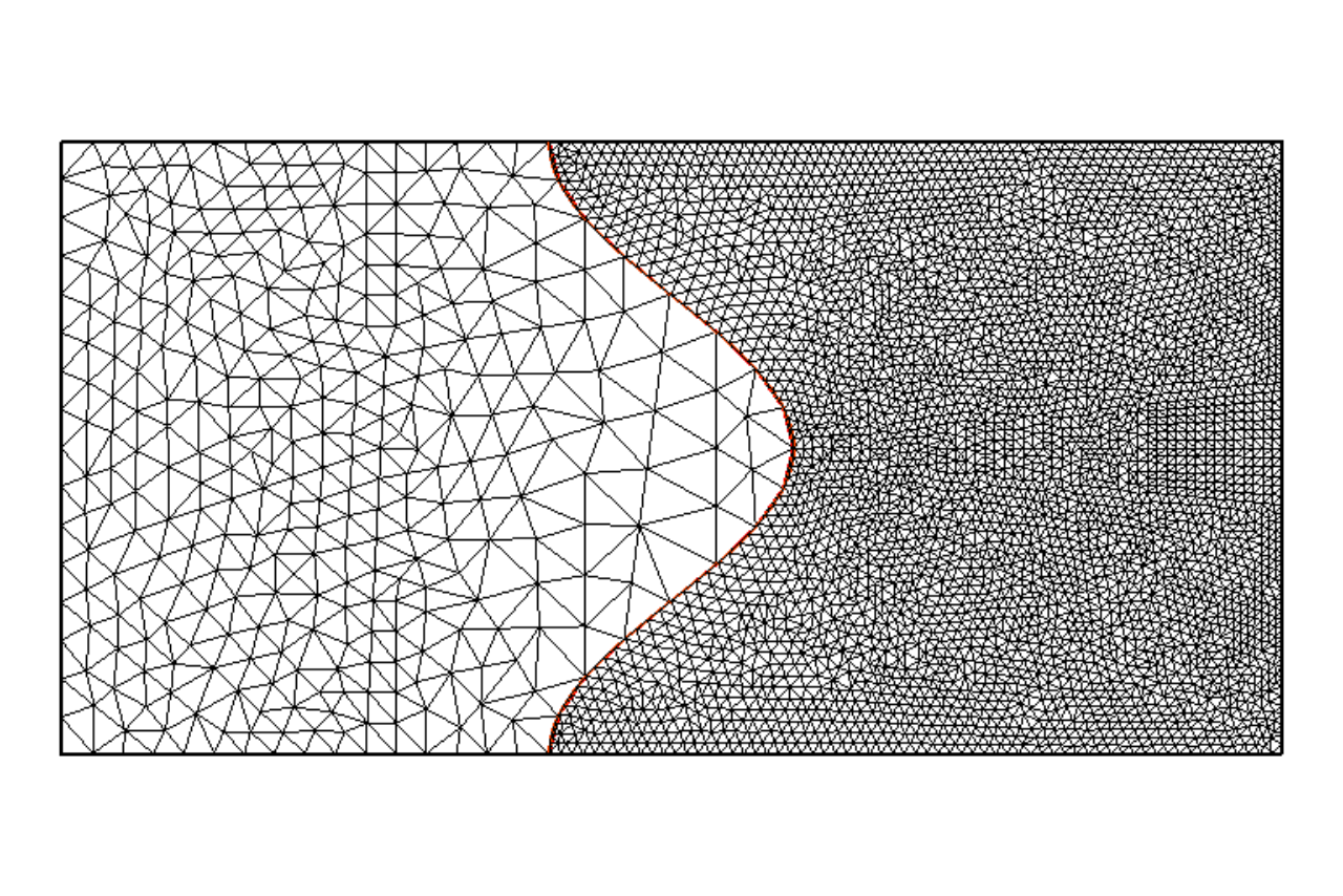
Refer to caption — Figure 5: An illustration of a spatially noncoincident mesh used in the numerical examples.

4.1 The Domain Decomposition Problem

For the sake of convenience, we set the Lamé parameters $(\lambda,\mu)=(1,1)$ on both subdomains. The coupled problem domain in this test problem is a rectangle that occupies the region $\Omega_{h}=\left[-1,1\right]\times[0,1]$ with discrete interfaces generated from the analytic representation $-\frac{1}{5}\cos(2\pi y)$ , where $y\in[0,1]$ at $x=0$ . $\Omega_{s,h}$ is taken to be the triangulation of the subdomain on the left side of the continuous interface, and $\Omega_{m,h}$ is taken to be the triangulation of the subdomain on the right side of the continuous interface.

4.1.1 The Linear Patch Test

In this numerical experiment, we determine whether (13) can recover the linear vector function $\mathbf{u}=\left[x+y,x+y\right]^{T}$ as an exact solution for the homogeneous problem. The results for some representative subdomain configurations are presented in Table 1. It is demonstrated that (13) for both spatially coincident and noncoincident interfaces. The relaxation parameter in the algorithm was set to $\omega=0.7$ .

$\#(\Gamma^{c}_{h,s})$	$\#(\Gamma^{c}_{h,m})$	$\\|\mathbf{u}-\mathbf{u}^{h}\\|_{L^{2}(\Omega_{h})}$	$K$
$25$	$25$	$2.4960\times 10^{-7}$	$28$
$100$	$100$	$2.2622\times 10^{-7}$	$26$
$25$	$50$	$3.0596\times 10^{-7}$	$28$
$25$	$100$	$3.1428\times 10^{-7}$	$29$
$50$	$25$	$2.7181\times 10^{-7}$	$27$
$100$	$25$	$4.8236\times 10^{-7}$	$36$

Table 1: Linear Patch Test. The iterative method (13) recovers the linear patch test.

4.1.2 Convergence to a Manufactured Solution

Here, we determine the rate of convergence of the solution of the discrete problem to the manufactured solution $\mathbf{u}=\left[\sin(\pi x)\sin(2\pi y),\sin(\pi x)\sin(2\pi y)\right]^{T}$ . First, we present the convergence results for the case where $\Gamma^{c}_{h,i}$ , $i=s,m$ , coincide, and then we shall present the convergence history for the spatially noncoincident cases, where the ratio between the number of elements on the master interface and the slave interface vary. We have demonstrated in the Tables 2–4 that the iterative method presented in the previous section converges optimally for piecewise linear Lagrange elements. An illustration of the convergence rate can be found in Fig. 7.

Figure 7:

H^{1}(\Omega_{h})

and

L^{2}(\Omega_{h})

convergence history illustration for the domain decomposition problem.

$\#(\Gamma^{c}_{h,s})$	$\#(\Gamma^{c}_{h,m})$	$h$	$\\|\mathbf{u}-\mathbf{u}^{h}\\|_{L^{2}(\Omega_{h})}$	$\\|\mathbf{u}-\mathbf{u}^{h}\\|_{H^{1}(\Omega_{h})}$	$K$
$8$	$8$	$0.244511$	$0.260548$	$3.22675$	$26$
$16$	$16$	$0.140988$	$0.0487357$	$1.48733$	$26$
$25$	$25$	$0.0948402$	$0.0203974$	$0.964635$	$22$
$50$	$50$	$0.0548697$	$0.00540889$	$0.480094$	$17$
$75$	$75$	$0.0350554$	$0.00255794$	$0.316482$	$17$
$100$	$100$	$0.0241639$	$0.00130554$	$0.233027$	$17$
$125$	$125$	$0.0220104$	$0.000741496$	$0.188069$	$18$
			$L^{2}(\Omega_{h})$ Rate	2.17
			$H^{1}(\Omega_{h})$ Rate	1.01

Table 2: Domain Decomposition Problem: Spatially Coincident Interface.

$\#(\Gamma^{c}_{h,s})$	$\#(\Gamma^{c}_{h,m})$	$h$	$\\|\mathbf{u}-\mathbf{u}^{h}\\|_{L^{2}(\Omega_{h})}$	$\\|\mathbf{u}-\mathbf{u}^{h}\\|_{H^{1}(\Omega_{h})}$	$K$
$8$	$16$	$0.244511$	$0.233747$	$2.48788$	$26$
$16$	$32$	$0.140988$	$0.0475133$	$1.17863$	$25$
$25$	$50$	$0.0948402$	$0.0220765$	$0.753572$	$22$
$50$	$100$	$0.0548697$	$0.00507153$	$0.367443$	$18$
$100$	$200$	$0.0241639$	$0.00126299$	$0.179719$	$18$
			$L^{2}(\Omega_{h})$ Rate	2.25
			$H^{1}(\Omega_{h})$ Rate	1.14

$\#(\Gamma^{c}_{h,s})$	$\#(\Gamma^{c}_{h,m})$	$h$	$\\|\mathbf{u}-\mathbf{u}^{h}\\|_{L^{2}(\Omega_{h})}$	$\\|\mathbf{u}-\mathbf{u}^{h}\\|_{H^{1}(\Omega_{h})}$	$K$
$16$	$8$	$0.29873$	$0.081574$	$2.69409$	$33$
$32$	$16$	$0.148393$	$0.0192996$	$1.24801$	$26$
$50$	$25$	$0.0830141$	$0.00662555$	$0.776856$	$23$
$100$	$50$	$0.0441468$	$0.00150745$	$0.39077$	$24$
$200$	$100$	$0.0222507$	$0.000557604$	$0.189376$	$22$
			$L^{2}(\Omega_{h})$ Rate	1.95
			$H^{1}(\Omega_{h})$ Rate	1.01

Table 3: Domain Decomposition Problem. Top:

(1:2)

slave : master ratio. Bottom:

(2:1)

slave : master ratio.

$\#(\Gamma^{c}_{h,s})$	$\#(\Gamma^{c}_{h,m})$	$h$	$\\|\mathbf{u}-\mathbf{u}^{h}\\|_{L^{2}(\Omega_{h})}$	$\\|\mathbf{u}-\mathbf{u}^{h}\\|_{H^{1}(\Omega_{h})}$	$K$
$8$	$32$	$0.244511$	$0.241335$	$2.39941$	$25$
$16$	$64$	$0.140988$	$0.0535691$	$1.08416$	$24$
$25$	$100$	$0.0948402$	$0.0235007$	$0.689027$	$23$
$50$	$200$	$0.0548697$	$0.00497135$	$0.334919$	$19$
$100$	$400$	$0.0241639$	$0.00126203$	$0.163256$	$18$
			$L^{2}(\Omega_{h})$ Rate	2.29
			$H^{1}(\Omega_{h})$ Rate	1.16

$\#(\Gamma^{c}_{h,s})$	$\#(\Gamma^{c}_{h,m})$	$h$	$\\|\mathbf{u}-\mathbf{u}^{h}\\|_{L^{2}(\Omega_{h})}$	$\\|\mathbf{u}-\mathbf{u}^{h}\\|_{H^{1}(\Omega_{h})}$	$K$
$32$	$8$	$0.29873$	$0.0513822$	$2.51413$	$36$
$64$	$16$	$0.148393$	$0.0094199$	$1.1693$	$31$
$100$	$25$	$0.0830141$	$0.00582067$	$0.728018$	$36$
$200$	$50$	$0.0441468$	$0.0019599$	$0.366355$	$52$
$400$	$100$	$0.0222507$	$0.00030831$	$0.160208$	$32$
			$L^{2}(\Omega_{h})$ Rate	1.85
			$H^{1}(\Omega_{h})$ Rate	0.98

Table 4: Domain Decomposition Problem. Top:

(1:4)

slave : master ratio. Bottom:

(4:1)

slave : master ratio.

4.2 Discontinuous Lamé Parameters

In this test problem, we consider the coupling problem (9) with Lamé parameters $(\lambda_{s},\mu_{s})=(2,1)$ and $(\lambda_{m},\mu_{m})=(2,1)$ . The coupled problem domain in this test case is the same as the domain considered in the previous subsection, i.e., a rectangle that occupies the region $\Omega_{h}=[-1,1]\times[0,1]$ with discrete interfaces generated from the analytic representation $-\frac{1}{5}\cos(2\pi y)$ , where $y\in[0,1]$ at $x=0$ . $\Omega_{s,h}$ is again taken to be the triangulation of the subdomain at the left side of the continuous interface, and $\Omega_{m},h$ is taken to be the triangulation of the subdomain on the right side of the continuous interface. We have set $\mathbf{f}_{s}=\left[10,10\right]^{T}$ and $\mathbf{f}_{m}=\left[-10,-10\right]^{T}$ and $\mathbf{u}_{s}=0$ on $\Gamma_{s,h}$ and $\mathbf{u}_{m}=0$ on $\Gamma_{m,h}$ . The relaxation parameter used in this numerical experiment was chosen to be $\omega=0.7$ . We test the rate of convergence of our iterative method against an “overkilled” solution, i.e., a discrete solution computed on a mesh size of $5.499\times 10^{-3}$ . This solution was computed monolithically using standard piecewise linear Lagrange elements.

From the numerical results gathered from this experiment, it is clear that the iterative method presented in the previous section is a general method that is second order accurate in $L^{2}(\Omega_{h})$ and first order accurate in $H^{1}(\Omega_{h})$ .

Figure 9:

H^{1}(\Omega_{h})

and

L^{2}(\Omega_{h})

convergence for the discontinuous Lamé parameter test problem.

$\#(\Gamma^{c}_{h,s})$	$\#(\Gamma^{c}_{h,m})$	$h$	$\\|\mathbf{u}-\mathbf{u}^{h}\\|_{L^{2}(\Omega_{h})}$	$\\|\mathbf{u}-\mathbf{u}^{h}\\|_{H^{1}(\Omega_{h})}$	$K$
$8$	$8$	$0.29873$	$0.0469285$	$0.446852$	$14$
$16$	$16$	$0.140988$	$0.0117446$	$0.195434$	$13$
$25$	$25$	$0.0948402$	$0.00415211$	$0.122464$	$12$
$50$	$50$	$0.0548697$	$0.00110825$	$0.0597868$	$14$
$75$	$75$	$0.0350554$	$0.000525341$	$0.0433184$	$15$
$100$	$100$	$0.0241639$	$0.000295744$	$0.0367863$	$15$
$125$	$125$	$0.0220104$	$0.000192478$	$0.0338451$	$16$
			$L^{2}(\Omega_{h})$ Rate	2.10
			$H^{1}(\Omega_{h})$ Rate	1.00

Table 5: Different Lamé Parameters: Spatially Coincident Interface.

$\#(\Gamma^{c}_{h,s})$	$\#(\Gamma^{c}_{h,m})$	$h$	$\\|\mathbf{u}-\mathbf{u}^{h}\\|_{L^{2}(\Omega_{h})}$	$\\|\mathbf{u}-\mathbf{u}^{h}\\|_{H^{1}(\Omega_{h})}$	$K$
$8$	$16$	$0.244511$	$0.0451623$	$0.375507$	$14$
$16$	$32$	$0.140988$	$0.0114271$	$0.167331$	$13$
$25$	$50$	$0.0948402$	$0.0036823$	$0.103027$	$13$
$50$	$100$	$0.0548697$	$0.00101088$	$0.0536388$	$15$
$100$	$200$	$0.0241639$	$0.00028725$	$0.0342972$	$16$
			$L^{2}(\Omega_{h})$ Rate	2.01
			$H^{1}(\Omega_{h})$ Rate	1.04

$\#(\Gamma^{c}_{h,s})$	$\#(\Gamma^{c}_{h,m})$	$h$	$\\|\mathbf{u}-\mathbf{u}^{h}\\|_{L^{2}(\Omega_{h})}$	$\\|\mathbf{u}-\mathbf{u}^{h}\\|_{H^{1}(\Omega_{h})}$	$K$
$16$	$8$	$0.29873$	$0.018827$	$0.316666$	$19$
$32$	$16$	$0.148393$	$0.00480391$	$0.150653$	$15$
$50$	$25$	$0.0830141$	$0.00178996$	$0.0903401$	$14$
$100$	$50$	$0.0441468$	$0.000512853$	$0.0460626$	$16$
$200$	$100$	$0.0222507$	$0.000153844$	$0.0325039$	$19$
			$L^{2}(\Omega_{h})$ Rate	1.86
			$H^{1}(\Omega_{h})$ Rate	0.90

Table 6: Different Lamé Parameters. Top:

(1:2)

slave : master ratio. Bottom:

(2:1)

slave : master ratio.

$\#(\Gamma^{c}_{h,s})$	$\#(\Gamma^{c}_{h,m})$	$h$	$\\|\mathbf{u}-\mathbf{u}^{h}\\|_{L^{2}(\Omega_{h})}$	$\\|\mathbf{u}-\mathbf{u}^{h}\\|_{H^{1}(\Omega_{h})}$	$K$
$8$	$32$	$0.244511$	$0.044073$	$0.354096$	$14$
$16$	$64$	$0.140988$	$0.0114338$	$0.162604$	$13$
$25$	$100$	$0.0948402$	$0.00356991$	$0.0996944$	$13$
$50$	$200$	$0.0548697$	$0.000985668$	$0.0517424$	$15$
$100$	$400$	$0.0241639$	$0.000286343$	$0.0332221$	$16$
			$L^{2}(\Omega_{h})$ Rate	2.21
			$H^{1}(\Omega_{h})$ Rate	1.04

$\#(\Gamma^{c}_{h,s})$	$\#(\Gamma^{c}_{h,m})$	$h$	$\\|\mathbf{u}-\mathbf{u}^{h}\\|_{L^{2}(\Omega_{h})}$	$\\|\mathbf{u}-\mathbf{u}^{h}\\|_{H^{1}(\Omega_{h})}$	$K$
$32$	$8$	$0.29873$	$0.0159833$	$0.284411$	$34$
$64$	$16$	$0.132189$	$0.00413673$	$0.126088$	$40$
$100$	$25$	$0.0830141$	$0.0013636$	$0.0812393$	$27$
$200$	$50$	$0.0441468$	$0.000467162$	$0.0427591$	$29$
$400$	$100$	$0.0222507$	$0.00011361$	$0.0317956$	$34$
			$L^{2}(\Omega_{h})$ Rate	1.91
			$H^{1}(\Omega_{h})$ Rate	0.87

Table 7: Different Lamé Parameters. Top:

(1:4)

slave : master ratio. Bottom:

(4:1)

slave : master ratio.

5 Conclusion

In this paper, we have described a coupling formulation for coupling the equations of linear elasticity in the discrete setting where the discrete interface is noncoincident. In addition, we have proposed an iterative solution method that solves this coupling formulation. In the numerical experiments presented in the numerical results section that the converged solution to our iterative solution method satisfies the expected error bounds for piecewise linear finite elements. The numerical results presented in the previous section implies that this method is applicable for both domain decomposition problems and interface coupling problems where the Lamé parameters differ on the problem subdomains.

In the monolithic formulation (9), we have approximated the Dirichlet subproblem with an oblique derivative problem. We anticipate that this approximation may also be used to improve the error bounds of finite element approximations on unfitted meshes, as was done in [2]. In addition, we anticipate that, in the future, we will generalize this method to $k$ –order polynomial approximation spaces and to time–dependent problems. A mathematical treatment on this method applied to the Poisson equation will be the topic of an upcoming work.

6 Appendix: Definition of the Zhang–Naga Gradient Recovery Operator

Let us first define the notion of an element patch. Let $z_{0}\in\mathcal{N}$ be a node in $\overline{\mathcal{T}}_{s,h}$ and $T\in\overline{\mathcal{T}}_{s,h}$ be a triangle in $\overline{\mathcal{T}}_{s,h}$ , then we can define an initial element patch as the following

\mathcal{K}^{0}_{z_{0}}=\left\{T\in\overline{\mathcal{T}}_{s,h};z_{0}\in T\right\}.

(18)

We can define the next level element patch as the following

\mathcal{K}^{1}_{z_{0}}=\left\{T\in\overline{\mathcal{T}}_{s,h};z_{\mathcal{K}^{0}_{z_{0}}}\in T\right\},

(19)

where $z_{\mathcal{K}^{0}_{z_{0}}}$ is a node that belongs to the triangles of $K^{0}_{z_{0}}$ . Through induction, we can set the $i^{th}$ level patch as

\mathcal{K}^{i}_{z_{0}}=\left\{T\in\overline{\mathcal{T}}_{s,h};z_{\mathcal{K}^{i-1}_{z_{0}}}\in T\right\},

(20)

where $z_{\mathcal{K}^{i-1}_{z_{0}}}$ is a node that belongs to the triangles of $K^{i-1}_{z_{0}}.$ We define the element patch as

\mathcal{K}_{z_{0}}=\left\{\mathcal{K}^{i}_{z_{0}};\textrm{card}(\mathcal{K}^{i}_{z_{0}})>6\textrm{ and }\textrm{card}(\mathcal{K}^{i-1}_{z_{0}})\leq 6\right\},

(21)

where, $\textrm{card}(\cdot)$ denotes the number of nodes in a set. Having defined an element patch, we can now define the local gradient recovery operator $G^{h}:V^{h}_{s}\rightarrow V^{h}_{s}\times V^{h}_{s}$ . Let $z_{0}$ and $\mathcal{K}_{z_{0}}$ again be a node in $\overline{\mathcal{T}}_{s,h}$ and its associated element patch respectively. Let $Z$ be the number of nodes in $\mathcal{K}_{z_{0}}$ excluding $z_{0}$ . In addition, let $z_{i}$ , $i\in[0,Z]$ be the nodes of the element patch and $(x_{i},y_{i})$ be the xy–coordinates of $z_{i}$ and $(\hat{x}_{i},\hat{y}_{i})=(x_{i}-x_{0},y_{i}-y_{0})$ be the coordinates centered around $z_{0}$ . Define

A_{z_{0}}=\left[\begin{array}[]{c}\mathbf{\hat{x}}_{0}^{T}\\ \mathbf{\hat{x}}_{1}^{T}\\ \vdots\\ \mathbf{\hat{x}}_{Z}^{T}\end{array}\right],\ \mathbf{\hat{x}}_{i}=\left[\begin{array}[]{c}1\\ \hat{x}_{i}\\ \hat{y}_{i}\\ \hat{x}_{i}^{2}\\ \hat{x}_{i}\hat{y}_{i}\\ \hat{y}_{i}^{2}\end{array}\right],\ \mathbf{c}_{z_{0}}=\left[\begin{array}[]{c}c_{0}\\ c_{1}\\ \vdots\\ c_{5}\end{array}\right],\ \textrm{ and }\mathbf{d}_{z_{0}}=\left[\begin{array}[]{c}v^{h}(z_{0})\\ v^{h}(z_{1})\\ \vdots\\ v^{h}(z_{Z})\end{array}\right].

(22)

The discrete quadratic least–squares fitting of a function $v^{h}\in V^{h}_{s}$ over the patch $\mathcal{K}_{z_{0}}$ can be performed by solving the least–squares problem

A_{z_{0}}^{T}A_{z_{0}}\mathbf{c}_{z_{0}}=A_{z_{0}}^{T}\mathbf{d}_{z_{0}}

(23)

for the coefficients $\mathbf{c}_{z_{0}}$ of the approximating polynomial and setting

p_{z_{0}}(x,y):=\mathbf{c}_{z_{0}}^{T}\mathbf{P},

(24)

where $\mathbf{P}=\left[1,x-x_{0},y-y_{0},(x-x_{0})^{2},(x-x_{0})(y-y_{0}),(y-y_{0})^{2}\right]^{T}$ . Now, we define $G^{h}_{z_{0}}$ , the local gradient recovery operator defined at node $z_{0}$ as

G^{h}_{z_{0}}u^{h}(z_{0}):=\nabla p_{z_{0}}(x_{0},y_{0}).

(25)

The global gradient recovery operator $G^{h}$ is a composite of all the local gradient recovery operators; for each node $z_{0}\in\mathcal{N}$ , set the nodal degree of freedom of $V^{h}_{s}\times V^{h}_{s}$ over $\overline{\mathcal{T}}_{s,h}$ to $G^{h}_{z_{0}}v^{h}(z_{0})$ .

Figure 10: An illustration of the element patch of a node

z_{0}\in\overline{\mathcal{T}}_{s,h}

Remark.

Computational implementation of $G^{h}$ is relatively simple due to the fact that $\nabla p_{z_{0}}(x_{0},y_{0})=[c_{1},c_{2}]^{T}$ at every node $z_{0}\in\mathcal{N}$ .

References

[1] Christine Bernardi. A new nonconforming approach to domain decomposition: the mortar element method. Nonliner Partial Differential Equations and Their Applications, 1994.
[2] Bernardo Cockburn and Manuel Solano. Solving dirichlet boundary–value problems on curved domains by extensions from subdomains. SIAM Journal on Scientific Computing, 2012.
[3] David Day and Pavel Bochev. Analysis and computation of a least-squares method for consistent mesh tying. Journal of Computational and Applied Mathematics, 218(1):21–33, 2008.
[4] Aukje de Boer, Alexander H van Zuijlen, and Hester Bijl. Comparison of conservative and consistent approaches for the coupling of non-matching meshes. Computer Methods in Applied Mechanics and Engineering, 197(49):4284–4297, 2008.
[5] Frédéric Hecht, Olivier Pironneau, A Le Hyaric, and K Ohtsuka. Freefem++ manual, 2005.
[6] TA Laursen and MW Heinstein. Consistent mesh tying methods for topologically distinct discretized surfaces in non-linear solid mechanics. International journal for numerical methods in engineering, 57(9):1197–1242, 2003.
[7] Nick Levine. Superconvergent recovery of the gradient from piecewise linear finite-element approximations. IMA Journal of numerical analysis, 5(4):407–427, 1985.
[8] Ahmed Naga and Zhimin Zhang. A posteriori error estimates based on the polynomial preserving recovery. SIAM Journal on Numerical Analysis, 42(4):1780–1800, 2004.
[9] ML Parks, L Romero, and P Bochev. A novel lagrange-multiplier based method for consistent mesh tying. Computer methods in applied mechanics and engineering, 196(35):3335–3347, 2007.
[10] Alfio Quarteroni and Alberto Valli. Domain decomposition methods for partial differential equations. Number CMCS-BOOK-2009-019. Oxford University Press, 1999.
[11] Andrea Toselli and Olof B Widlund. Domain decomposition methods: algorithms and theory, volume 34. Springer, 2005.
[12] Barbara I Wohlmuth. A mortar finite element method using dual spaces for the lagrange multiplier. SIAM journal on numerical analysis, 38(3):989–1012, 2000.
[13] Zhimin Zhang and Ahmed Naga. A new finite element gradient recovery method: Superconvergence property. SIAM Journal on Scientific Computing, 26(4):1192–1213, 2005.
[14] OC Zienkiewicz and JZ Zhu. The superconvergent patch recovery (spr) and adaptive finite element refinement. Computer Methods in Applied Mechanics and Engineering, 101(1):207–224, 1992.
[15] Olgierd Cecil Zienkiewicz and Jian Zhong Zhu. The superconvergent patch recovery and a posteriori error estimates. part 1: The recovery technique. International Journal for Numerical Methods in Engineering, 33(7):1331–1364, 1992.

A Coupling Approach for Linear Elasticity Problems with Spatially Noncoincident Interfaces

Abstract

1 Introduction

2 Statement of the Interface Problem

2.1 The Continuous Interface Problem

2.2 Finite Element Approximation

2.2.1 Spatially Noncoincident Interfaces

Taylor Series Expansion Operators

A Noncoincident Interface Formulation

Remark.

Linear Consistency

Proposition 1.

Proof.

Remark (Second Order Accuracy).

3 An Iterative Solution Method

Remark.

3.1 Implementation

Defining ϕs​m\phi_{sm} and ϕm​s\phi_{ms}

Remark.

The Dirichlet Subproblem

The Neumann Subproblem

A Complete Description of the Algorithm

Algorithm 1 (Modified Dirichlet–Neumann).

4 Numerical Results

4.1 The Domain Decomposition Problem

4.1.1 The Linear Patch Test

4.1.2 Convergence to a Manufactured Solution

4.2 Discontinuous Lamé Parameters

5 Conclusion

6 Appendix: Definition of the Zhang–Naga Gradient Recovery Operator

Remark.

References

Defining $\phi_{sm}$ and $\phi_{ms}$