Multitask Learning using Task Clustering with Applications to Predictive Modeling and GWAS of Plant Varieties
Abstract.
Inferring predictive maps between multiple input and multiple output variables or tasks has innumerable applications in data science. Multi-task learning attempts to learn the maps to several output tasks simultaneously with information sharing between them. We propose a novel multi-task learning framework for sparse linear regression, where a full task hierarchy is automatically inferred from the data, with the assumption that the task parameters follow a hierarchical tree structure. The leaves of the tree are the parameters for individual tasks, and the root is the global model that approximates all the tasks. We apply the proposed approach to develop and evaluate: (a) predictive models of plant traits using large-scale and automated remote sensing data, and (b) GWAS methodologies mapping such derived phenotypes in lieu of hand-measured traits. We demonstrate the superior performance of our approach compared to other methods, as well as the usefulness of discovering hierarchical groupings between tasks. Our results suggest that richer genetic mapping can indeed be obtained from the remote sensing data. In addition, our discovered groupings reveal interesting insights from a plant science perspective.
Keywords:
High-throughput phenotyping, Multitask learning, Convex clustering, Sparse linear regression1. Introduction
Several problems in data science necessitate discovery of a predictive mapping from input to output data, such that it can be generalized to new inputs. In many applications, there can be more than one output variable and they can be related to each other, and it is also desirable for the mappings to have some structure. Multi-output regression models generalize single-output regression models to learn predictive relationships between multiple input and multiple output variables, also referred to as tasks (Borchani et al., 2015). Multi-task learning attempts to learn several the inference tasks simultaneously, and the assumption here is that an appropriate sharing of information can benefit all the tasks (Caruana, 1998; Obozinski et al., 2006). There are several ways to define task-relatedness; the parameters can be close to each other (Evgeniou and Pontil, 2004), they can share a common prior (Daumé III, 2009), or they can share a common latent feature representation (Caruana, 1998). We will only focus on multi-task learning under the linear sparse modeling framework.
The implicit assumption that sharing all features for all tasks can be excessive and can ignore the underlying specificity of the mappings. There have been several extensions to multi-task learning that address the problem of how to, and with whom to share between the tasks (Jalali et al., 2010; Kang et al., 2011; Kim and Xing, 2010; Swirszcz and Lozano, 2012; Jacob et al., 2009; Kumar and Daume III, 2012). The authors in (Jalali et al., 2010) propose a dirty model for feature sharing among tasks, wherein a linear superposition of two sets of parameters - one that is common to all tasks, and one that is task-specific is used. A variant of this was proposed in (Swirszcz and Lozano, 2012) with elementwise product between the two parameter sets. The approach proposed in (Kumar and Daume III, 2012) learns to share by defining a set of basis task parameters and posing the task-specific parameters as a sparse linear combination of these. In (Jacob et al., 2009) and (Kang et al., 2011), the authors assume that the tasks are clustered into groups and proceed to learn the group structure along with the task parameters using a convex and an integer quadratic program respectively. In contrast to the above approaches, (Kim and Xing, 2010) leverages a predefined tree structure among the output tasks (e.g. using hierarchical agglomerative clustering) and imposes group regularizations on the task parameters based on this tree.
In this work, we propose to simultaneously learn the task parameters of a multi-task linear regression model as well as the structured relationship between the tasks in a fully supervised manner. We assume that the task parameters follow a general hierarchical tree structure, and hence this approach learns the full task sharing hierarchy automatically. We adopt such a structure as it is natural to model task relatedness, similarly as in hierarchical clustering and it is also easily interpretable. Our framework is motivated by several applications such as in genome wide association analysis with multiple output phenotypes (Schifano et al., 2013), and predictive modeling of plant traits with remote sensed data in automated phenotyping (Ramamurthy et al., 2016) to name a few. To the best of our knowledge, ours is the first attempt in the literature to learn a hierarchical task clustering structure in a supervised manner. Our proposed approach constrains the parameters of each task to be sparse and incorporates an additional regularization on the task parameters inspired by convex clustering (Hocking et al., 2011a). Similar to convex clustering, a continuous regularization path of solutions can be obtained and each point in the path corresponds to a threshold for cutting the task parameter tree.
The main contributions of this paper are as follows. We propose a structured multi-task learning estimator that can learn a tree structure among the tasks while simultaneously estimating the task parameters. We present a proximal decomposition approach to efficiently solve the resulting convex problem, and show its numerical convergence. We provide statistical guarantees and study the asymptotic properties of our estimator. Our approach is validated empirically on simulated data. We also explore the applications of the proposed method in two high-throughput phenotyping problems: (a) predictive modeling of plant traits using large-scale and automated remote sensing data, and (b) Genome-Wide Association Studies (GWAS) mapping such derived phenotypes in lieu of hand-measured traits. Initial results are promising and show that our method produces high predictive accuracy while revealing groupings that are insightful.
2. Background
Multi-task Learning.
Consider the multi-task linear regressions: for each task
for where , , and . Suppose we are given i.i.d. samples for task . We will overload notation and collate these observations using vector notation as:
where , , and . Throughout the paper, we concatenate parameters in columns to form (i.e. -th column, , is ), and assume that all tasks have the same number of observations for notational simplicity. Note that in the multi-response model where the design matrix is shared across all tasks, we have in a simpler form with , and . Generally, multi-task learning solves the following optimization problem
| (1) |
where the penalty on the task parameters encourages information sharing.
Convex Clustering.
Clustering is a fundamental unsupervised problem which is broadly used in many scientific applications. Given data points (our choice of notation here is deliberate for the next section), Lindsten et al. (2011); Hocking et al. (2011b) propose a convex optimization problem for clustering points:
| (2) |
where is a positive tuning parameter, is a nonnegative weight. Note that for the second term, other penalties rather than norm have been also considered. As discussed in Chi and Lange (2015), each point constitutes an independent cluster when is small enough, however, as increases, the cluster centers start to combine.
3. Multitask Learning with Task Clustering
Our goal is to jointly infer (a) the linear regression parameter matrix allowing for high-dimensional sampling settings where the number of observations is possibly much larger than the problem dimension ; (b) a general hierarchical tree structure among the tasks.
To accomplish this goal, we propose to solve the following regularized regression problem:
| (3) |
The above formulation has three terms. The first term is the squared loss. While we focus on linear regression, our approach can be readily generalized and employ other loss functions such as the logistic loss, the loss, etc.
The second term encourages the sparsity of the regression coefficient matrix . Clearly, this can be generalized to a more sophisticated sparsity structure, e.g., group sparsity, based on the needs of the application.
The third term encourages tasks to share the same value of their parameter vectors. It can be viewed as a generalization of the fused lasso penalty (Tibshirani et al., 2005) wherein we fuse the parameter vectors rather than the scalar coefficients. This is identical to the convex clustering penalty (Chi and Lange, 2015) in (2), but it forms clusters for task parameters rather than data points. Hence, brought into our framework, this penalty induces clustering of task parameters, effectively learning a hierarchical tree of these parameters.
and are tuning parameters that control the degree of individual task sparsity and task sharing respectively. As in (2), when is small enough, each task parameter is allowed to focus on minimizing individual loss function . However, as increases, the relative importance of third term increases and task parameters start to combine. In this sense, our formulation (3) can be viewed as supervised clustering problem. Setting these parameters is essential to decide the behavior of (3), and they can be tuned e.g. via cross validation. Finally, are optional non-negative weights that can be imposed to reflect prior knowledge on the degree of relatedness between each pair of tasks.
The choice of the weights can dramatically affect the complexity of the minimization problem. Typically it is desirable to have sparse weights : only a small portion of them are non-zero. As suggested in (Chi and Lange, 2015), we can set , where is 1 if is among ’s -nearest-neighbors or vice versa and 0 otherwise. The constant is nonnegative; corresponds to uniform weights for all neighbors.
3.1. Optimization via Proximal Decomposition
In this section we describe an optimization algorithm to solve our formulation (3). Since the task loss function for linear regression problem is convex, our formulation overall is also convex in , so it can be solved using modern convex optimization approaches. The story here can be trivially generalized to general loss function beyond squared loss, as long as it is convex.
Here we adopt the proximal decomposition method introduced in (Combettes and Pesquet, 2008). This is an efficient algorithm for minimizing the summation of several convex functions. Our objective function involves such functions (Note that is usually sparse so we do not have to deal with terms):
At a high level, the algorithm iteratively applies proximal updates with respect to the above functions. We now describe the details of the algorithm as summarized in Algorithm 1. We stack the regression matrix into a column vector . In the algorithm denote the iteration number. Each , or is a dimensional column vector, corresponding to our parameter . The procedure has two additional parameters and In practice we can set for each iteration ‘prox’ denotes the proximal operator: where and are vectors.
We iteratively apply the proximal updates for and until convergence. The specific update rules are as follows.
- •
Update for : Let For each , we have
This step corresponds to the closed-form formula of a ridge regression problem. For very large we can employ efficient approaches such as (McWilliams et al., 2014) and (Lu and Foster, 2014).
- •
Update for : Let For each , ,
- •
Updates for : Let For each with , let ,
3.2. Numerical Convergence
The following proposition characterizes the convergence of Algorithm 1. It is a direct consequence of Theorem 3.4. in (Combettes and Pesquet, 2008).
Proposition 3.1.
The proof is presented in the appendix.
4. Theoretical Guarantees
In this section, we provide the asymptotic properties of our estimators (3) that can be understood as the extension of those for vanilla Lasso (Knight and Fu, 2000) and fused Lasso (Tibshirani et al., 2005). Following the strategy in (Knight and Fu, 2000; Tibshirani et al., 2005), we assume in the main statement that the feature dimension is fixed as the number of samples approaches infinity. Though restrictive, this setting is more effective to illustrate the dynamics of methods.
Before providing the main statement, we first introduce some quantities for clear representation. Let be the population minimizer of the risk: . Given the population or target parameter , we define two functions corresponding to two types of regularizers. Specifically, let be the limit definition of derivative for individual regularization terms: , where . Then, can be rewritten as
| (4) |
where is the indicator function, and (and respectively) is the -th feature weight of the target parameter . Similarly, let be the limit definition of derivative for a single fusion term , defined as
Then, it can be easily verified that the sum of over all fusion terms is written as
| (5) |
Armed with these quantities, the following theorem characterizes the limiting distribution on optimal solution of (3), .
Theorem 4.1.
Given the construction of (4) and (5), the proof of Theorem 4.1 follows easily from the line of previous works e.g. (Knight and Fu, 2000) or (Tibshirani et al., 2005).
The theorem confirms that the joint limiting distribution of will have probability concentrated on the line if , and , in addition to a lasso-type effect (as in (Knight and Fu, 2000)) on univariate limiting distributions when .
Note that in case of a ‘multi-output’ setting where the design matrix is shared across all tasks, Theorem 4.1 holds with the simpler form of : .
Note also that the extension of Theorem 4.1 beyond least squares
where is a general loss function (e.g. logistic loss) is also trivially attainable following (Rocha et al., 2009).
5. Simulated Data Experiments

As a sanity check, we evaluate our approach on synthetic datasets and compare with the following baselines:
- •
Single task: a baseline approach, where the tasks are learned separately via Lasso.
- •
No group MTL (Obozinski et al., 2006): the traditional multitask approach using group lasso penalty, where all tasks are learned jointly and the same features are selected across tasks.
- •
Pre-group MTL: Given the true number of groups, first partition the tasks purely according to the correlation among responses and then apply No group MTL in each cluster.
- •
Kang et al (Kang et al., 2011): Mixed integer program learning a shared feature representations among tasks, while simultaneously determining “with whom” each task should share. We used the code provided by the authors of (Kang et al., 2011) and used the true number of tasks.
- •
Tree-guided group Lasso (Kim and Xing, 2010): Employs a structured penalty function induced from a predefined tree structure among responses, that encourages multiple correlated responses to share a similar set of covariates. We used the code provided by the authors of (Kim and Xing, 2010) where the tree structure is obtained by running a hierarchical agglomerative clustering on the responses.
We consider samples, features, and three groups of tasks. Within each group there are 5 tasks whose parameter vectors are sparse and identical to each other. We generate independent train, validation, and test sets. For each method, we select the regularization parameters using the validation sets, and report the root-mean-squared-error (RMSE) of the resulting models on the test sets. We repeat this procedure 5 times. The results are reported in Table 1. From the table we can see that the Single task method has the largest RMSE as it does not leverage task relatedness; No group MTL has slightly better RMSE; both Kang et al. and Tree guided group Lasso get some improvement by considering structures among tasks; Pre-group MLT achieves a better result, mainly because it is given the true number of groups and for these synthetic datasets it is quite easy to obtain good groups via response similarity, which might not necessarily be the case with real data and when the predictors differ from task to task. Our method achieves the smallest RMSE, outperforming all approaches compared. We also report the running times of each method, where we fix the tolerance parameters to for comparison. Though the timing for each method could always be improved using more effective implementations, the timing result reflect the algorithmic simplicity of the steps in our approach compare to e.g. the mixed integer program of (Kang et al., 2011).
| Method | RMSE | std | time |
|---|---|---|---|
| Single task | 5.665 | 0.131 | 0.02 |
| No group multitask learning | 5.520 | 0.115 | 0.05 |
| Pre-group multitask learning | 5.256 | 0.117 | 0.10 |
| Kang et al | 5.443 | 0.096 | |
| Tree guided group Lasso | 5.448 | 0.127 | 0.03 |
| Ours | 4.828 | 0.117 | 0.16 |
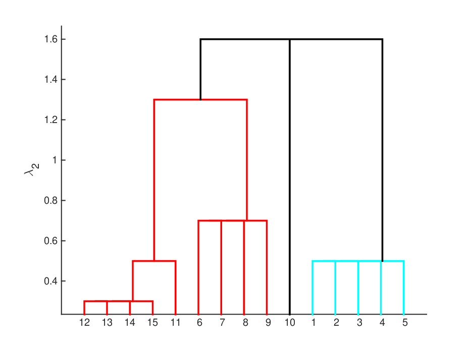
An example of tree structure learnt by our approach is shown in Figure 2. It is contrasted with Figure 2, which depicts the structure obtained a-posteriori by performing hierarchical clustering on the regression matrix learnt by Single Task. The simulation scenario is the same as before except that the non-zero coefficients in each true group are not equal but sampled as where denote the normal distribution. As can be seen from Figure 2, no matter what is, our approach never makes a mistake in the sense that it never puts tasks from different true groups in the same cluster. For our approach recognizes the true groups. As becomes very large there are no intermediary situation where two tasks are merged first. Instead all tasks are put in the same cluster. We see tasks merge first in group and merge first in group This corresponds to the fact that tasks have largest correlation among group and has largest correlation among group We can see in Figure 2 that for Single Task post clustering, task 10 does not merge with
Impact of the weights
One might argue that our approach relies on “good” weights among tasks. However, it turns out that it is quite robust to the weights. Recall that we select the weight by -nearest-neighbors. In this synthetic dataset, we have 5 tasks in each group so the most natural way is to set . We also try setting and see how this affects the result. The test RMSEs for different ’s are given in Table 2. From the table we see that although the best performance is when we select , our method is quite robust to the choice of weights, especially when is smaller than the natural one. When is large the result gets slightly worse, because now we cannot avoid positive weights across groups. But even if it is slightly worse, our method is still competitive.
| 2 | 3 | 4 | 5 | 6 | |
|---|---|---|---|---|---|
| RMSE | 4.847 | 4.836 | 4.828 | 4.896 | 4.928 |
6. Applications to Predictive Modeling and GWAS of Plant Varieties
We choose high throughput phenotyping and GWAS with real data obtained from plants to demonstrate the real-world utility of our approach. Accurate phenotyping of different crop varieties is a crucial yet traditionally a time-consuming step in crop breeding requiring manual survey of hundreds of plant varieties for the traits of interest. Recently, there has been a surge in interest and effort to develop automated, high-throughput remote sensing systems (Tuinstra et al., 2016) for trait development and genome wide association studies. The typical workflow of such systems is illustrated in Figure 3. Machine learning approaches are used to learn mappings between features obtained from remotely sensed images (e.g., RGB, hyperspectral, LiDAR, thermal) of plants as input and the manually collected traits (e.g., plant height, stalk diameter) as outputs. Genetic mapping is performed either with the inferred traits or directly with the features from remote sensing data.

We consider two specific problems from this pipeline: (a) predictive modeling of plant traits using features from remote sensed data (Section 6.1), (b) GWAS using the remote sensing data features (Section 6.2). Both these problems have unique challenges as discussed later. We apply our proposed multitask learning approach to automatically discover hierarchical groupings of output tasks, and learn differentiated models for the different groups while sharing information within groups. Apart from providing an improved predictive accuracy, the discovered groupings reveal interesting and interpretable relations between the tasks. The data used in the two experiments were collected in experimental fields in Summer-Fall 2015 and Summer-Fall 2016 respectively.

| Method | RMSE | std |
|---|---|---|
| Single model | 44.39 | 6.55 |
| No group multitask learning | 36.94 | 6.10 |
| Kang et al | 37.55 | 7.60 |
| Ours | 33.31 | 5.10 |
6.1. Trait Prediction from Remote Sensed Data
The experimental data consists of varieties of the sorghum crop planted in replicate plot locations. From the RGB and hyperspectral images of each plot, we extract features of length . Hence , , and . The presence of multiple varieties with replicates much smaller in number than predictors poses a major challenge: Building separate models for each variety is unrealistic, while a single model does not fit all. This is where our hierarchical grouping and modeling approach provides the flexibility to share information that leads to learning at the requisite level of robustness.
We have 3 different responses: plant height, stalk diameter, and stalk volume so we get 3 tree structures. The 3 trees are given in Figure 4, Figure 7 and Figure 7. The cluster provide some interesting insights from a plant science perspective. As highlighted in Figure 4, for predictive models of height, thicker medium dark plants are grouped together. Similarly for thinner tall dark plants, and thick tall plants with many light leaves. Figure 7 and Figure 7 are quite similar, which makes sense, since stalk diameter and stalk volume are highly correlated. In terms of stalk, we can see variety 12 is very different from others. It corresponds to tall thin plants with few small dark leaves.
Bin 2
Bin 3
Bin 4
Bins 1,5-10
Bin 2
Bin 3
Bin 4
Bins 1,5-10
In terms of predictive accuracy comparison, we focus on predictive plant height. We perform 6-folds CV where in each fold we make sure to include one sample from each variety. As we only have sample per variety (i.e. per task), it is unrealistic to learn separate models for each variety. Due to the limited sample size we focus on assessing the quality of the groupings of various methods as follows. For each CV split, we first learn a grouping using a comparison method and then treat all the samples within a group as i.i.d and estimate their regression coefficients using Lasso. We compare the groupings of (i) our approach (ii) Kang et al (iii) learning a single predictive model using Lasso, treating all the varieties as i.i.d. (iv) learning a traditional multitask model using Group Lasso (each variety form a separate group). The results are reported in Table 3, which indicate the superior quality of our groupings in terms of improving predictive accucacy.
6.2. GWAS dataset
In the second dataset, we use SNP data from 850 varieties as input for GWAS. We considered SNPs (features). There are plots (observations), each containing a single variety. The output data is the histogram of photogrammetrically derived heights obtained from RGB images of the plots. We consider bins, and each bin is treated as a task. Therefore, . It has been demonstrated that height histograms describe the structure of the plants in the plot and are hence powerful predictors of various traits (Ramamurthy et al., 2016). Therefore it is worthwhile performing genomic mapping using them bypassing trait prediction. Since it is reasonable to expect the neighboring bins of the histograms to be correlated, our approach for hierarchical task grouping will result in an improved association discovery.
For this dataset, the Kang et al. method did not scale to handle the amount of features. In general, we noticed that this algorithm is quite unstable, namely the task membership keep changing at each iteration especially as the problem dimensionality becomes large. The tree structure obtained by our method is given in Figure 7. Please note that the -axis in the figure is We notice that bins merge quickly while bins {2,3,4} merge when is extremely large. Note that the distance from bin 5 to bin 4 is much larger, compared to the distance from bin 7 to bin 5 (while in the figure it looks similar due to logarithmic scale. Bins are rarely populated. They all have small coefficients and merge together quickly; while more populated bins tend to merge later.
We zoom in on two locations on the genome: one on chromosome 7 between positions 5.5e7 and 6.2e7 (bp) and the other on chromosome 9 between positions 5.3e7 and 6e7 (bp). Notice that selected SNPs differ from one histogram bin group to another. Selected SNPs on chromosome 7 co-localize with ground truth (in particular with Dwarf3 gene). On chromosome 9, bin mapping identifies new regions (in addition to Dwarf1), possibly related to canopy closure, leaf distribution, flowering, and other plot-wide characteristics. As future work we plan to assess the statistical significance of the uncovered association and validate them further with domain experts.
7. Conclusion
In this paper we proposed a multitask learning approach that jointly learns the task parameters and a tree structure among tasks, in a fully automated, data-driven manner. The induced tree structure is natural for modeling task-relatedness and it is also easily interpretable. We developed an efficient procedure to solve the resulting convex problem and proved its numerical convergence. We also explored the statistical properties of our estimator. Using synthetic data, we demonstrated the superiority of our approach over comparable methods in terms of RMSE as well as inference of underlying task groups. Experiments with real-world high throughput phenotyping data illustrated the practical utility of our approach in an impactful application. In the future, we will explore other structured sparsity penalties, generalize the loss function to be other than squared and pursue the applications of our method to high-throughput phenotyping further.
Appendix A Proof of Proposition 3.1
We need to check that the conditions in Theorem 3.4 in (Combettes and Pesquet, 2008) are satisfied in our case:
Let be the domain of which can be set as . Let be a nonempty convex subset of , the strong relative interior of is
where , and is the closure of span .
Now we check the conditions. For (i), goes to infinity means goes to infinity, and then we know goes to infinity. Therefore (i) holds.
For (ii), we do not have any restriction on , so the right hand side is just , hence (ii) holds.
Therefore, the proposition follows according to Theorem 3.4 of (Combettes and Pesquet, 2008).
Acknowledgements.
The authors acknowledge the contributions of the Purdue and IBM project teams for field work, data collection/processing and discussions. The information, data, or work presented herein was funded in part by the Advanced Research Projects Agency-Energy (ARPA-E), U.S. Department of Energy, under the Award Number DE-AR0000593. The views and opinions of authors expressed herein do not necessarily state or reflect those of the United States Government or any agency thereof.References
- Borchani et al. (2015) Hanen Borchani, Gherardo Varando, Concha Bielza, and Pedro Larrañaga. 2015. A survey on multi-output regression. Wiley Interdisciplinary Reviews: Data Mining and Knowledge Discovery 5, 5 (2015), 216–233.
- Caruana (1998) Rich Caruana. 1998. Multitask learning. In Learning to learn. Springer, 95–133.
- Chi and Lange (2015) Eric C. Chi and Kenneth Lange. 2015. Splitting methods for convex clustering. Journal of Computational and Graphical Statistics 24, 4 (2015), 994–1013.
- Combettes and Pesquet (2008) Patrick L Combettes and Jean-Christophe Pesquet. 2008. A proximal decomposition method for solving convex variational inverse problems. Inverse problems 24, 6 (2008), 065014.
- Daumé III (2009) Hal Daumé III. 2009. Bayesian multitask learning with latent hierarchies. In Proceedings of the Twenty-Fifth Conference on Uncertainty in Artificial Intelligence. AUAI Press, 135–142.
- Evgeniou and Pontil (2004) Theodoros Evgeniou and Massimiliano Pontil. 2004. Regularized multi–task learning. In Proceedings of the tenth ACM SIGKDD international conference on Knowledge discovery and data mining. ACM, 109–117.
- Hocking et al. (2011a) Toby Dylan Hocking, Armand Joulin, Francis Bach, and Jean-Philippe Vert. 2011a. Clusterpath an algorithm for clustering using convex fusion penalties. In 28th international conference on machine learning. 1.
- Hocking et al. (2011b) Toby Dylan Hocking, Armand Joulin, Francis Bach, and Jean-Philippe Vert. 2011b. Clusterpath An Algorithm for Clustering using Convex Fusion Penalties. In International Conference on Machine learning (ICML).
- Jacob et al. (2009) Laurent Jacob, Jean-philippe Vert, and Francis R Bach. 2009. Clustered multi-task learning: A convex formulation. In Advances in neural information processing systems. 745–752.
- Jalali et al. (2010) Ali Jalali, Sujay Sanghavi, Chao Ruan, and Pradeep K Ravikumar. 2010. A dirty model for multi-task learning. In Advances in Neural Information Processing Systems. 964–972.
- Kang et al. (2011) Zhuoliang Kang, Kristen Grauman, and Fei Sha. 2011. Learning with whom to share in multi-task feature learning. In Proceedings of the 28th International Conference on Machine Learning (ICML-11). 521–528.
- Kim and Xing (2010) Seyoung Kim and Eric P. Xing. 2010. Tree-Guided Group Lasso for Multi-Task Regression with Structured Sparsity. In Proceedings of the 27th International Conference on Machine Learning (ICML-10). 543–550.
- Knight and Fu (2000) Keith Knight and Wenjiang Fu. 2000. Asymptotics for lasso-type estimators. Annals of Statistics 28 (2000), 1356–1378.
- Kumar and Daume III (2012) Abhishek Kumar and Hal Daume III. 2012. Learning task grouping and overlap in multi-task learning. arXiv preprint arXiv:1206.6417 (2012).
- Lindsten et al. (2011) Fredrik Lindsten, Henrik Ohlsson, and Lennart Ljung. 2011. Just Relax and Come Clustering! A Convexication of k-Means Clustering. In Tech. rep. Linköpings universitet.
- Lu and Foster (2014) Yichao Lu and Dean P Foster. 2014. Fast ridge regression with randomized principal component analysis and gradient descent. arXiv preprint arXiv:1405.3952 (2014).
- McWilliams et al. (2014) Brian McWilliams, Christina Heinze, Nicolai Meinshausen, Gabriel Krummenacher, and Hastagiri P Vanchinathan. 2014. LOCO: Distributing ridge regression with random projections. stat 1050 (2014), 26.
- Obozinski et al. (2006) Guillaume Obozinski, Ben Taskar, and Michael Jordan. 2006. Multi-task feature selection. Statistics Department, UC Berkeley, Tech. Rep 2 (2006).
- Ramamurthy et al. (2016) K.N. Ramamurthy, Z. Zhang, A. M. Thompson, F. He, M. M. Crawford, A. F. Habib, C. F. Weil, and M. R. Tuinstra. 2016. Predictive Modeling of Sorghum Phenotypes with Airborne Image Features. In Proc. of KDD Workshop on Data Science for Food, Energy, and Water.
- Rocha et al. (2009) Guilherme V. Rocha, Xing Wang, and Bin Yu. 2009. Asymptotic distribution and sparsistency for l1-penalized parametric M-estimators with applications to linear SVM and logistic regression. ArXiv preprint (2009).
- Schifano et al. (2013) Elizabeth D Schifano, Lin Li, David C Christiani, and Xihong Lin. 2013. Genome-wide association analysis for multiple continuous secondary phenotypes. The American Journal of Human Genetics 92, 5 (2013), 744–759.
- Swirszcz and Lozano (2012) Grzegorz Swirszcz and Aurelie C Lozano. 2012. Multi-level lasso for sparse multi-task regression. In Proceedings of the 29th International Conference on Machine Learning (ICML-12). 361–368.
- Tibshirani et al. (2005) Robert Tibshirani, Michael Saunders, Saharon Rosset, Ji Zhu, and Keith Knight. 2005. Sparsity and smoothness via the fused lasso. Journal of the Royal Statistical Society Series B (2005), 91–108.
- Tuinstra et al. (2016) M. R. Tuinstra et al. 2016. Automated Sorghum Phenotyping and Trait Development Platform. In Proc. of KDD Workshop on Data Science for Food, Energy, and Water.