Conditional Equivalence Testing: an alternative remedy for publication bias
Abstract
We introduce a publication policy that incorporates “conditional equivalence testing” (CET), a two-stage testing scheme in which standard NHST is followed conditionally by testing for equivalence. The idea of CET is carefully considered as it has the potential to address recent concerns about reproducibility and the limited publication of null results. In this paper we detail the implementation of CET, investigate similarities with a Bayesian testing scheme, and outline the basis for how a scientific journal could proceed to reduce publication bias while remaining relevant.
October, 2017
Keywords: Null Hypothesis Significance Testing, reliability, equivalence testing, non-inferiority testing, Bayesian testing, statistical power, confidence intervals
1 Introduction
Poor reliability, within many scientific fields, is a major concern for researchers, scientific journals and the public at large. In a highly cited essay, Ioannidis ((2005)) uses Bayes theorem to claim that more than half of published research findings are false. While not all agree with the extent of this conclusion, the argument raises concerns about the trustworthiness of science, amplified by a disturbing prevalence of scientific misconduct, Fanelli ((2009)). That the reliability of a result may be substantially lower than its -value suggests has been “underappreciated” (Goodman & Greenland, (2007)), to say the least.
To address this problem, some journal editors have taken radical measures (e.g. Trafimow & Marks ((2015))), while the reputation of researchers and the credibility of the science they generate are tarnished (Wasserstein & Lazar, (2016)). The foundational premise of null hypothesis significance testing (NHST) is now in question11 1 To be clear, NHST has long been controversial (Nickerson, (2000); Harlow et al., (2016)) but this controversy has recently been renewed. (Lash, (2017); Hofmann, (2016); Szucs & Ioannidis, (2016); Cumming, (2014)), and the usefulness of the -value vigorously debated (Lew, (2013); Chavalarias et al., (2016); Gelman, (2013)).
The limited publication of null results is certainly one of the most substantial factors contributing to low reliability. Whether due to a reluctance of journals to publish null results or to a reluctance of investigators to submit their null research (Dickersin et al., (1992); Reysen, (2006)), the consequence is severe publication bias; see Franco et al. ((2014)) and Doshi et al. ((2013)). Despite repeated warnings, publication bias persists and, to a certain degree, this is understandable. Accepting a null result can be difficult, owing to the well-known fact that “absence of evidence is not evidence of absence” (Hartung et al., (1983); Altman & Bland, (1995)). As Greenwald ((1975)) writes: “it is inadvisable to place confidence in results that support a null hypothesis because there are too many ways (including incompetence of the researcher), other than the null hypothesis being true, for obtaining a null result.” Indeed, this is the foremost critique of NHST, that it cannot provide evidence in favour of the null hypothesis. The commonly held belief that for non-significant result to show high “retrospective power” (Zumbo & Hubley, (1998)) implies support in favour of the null, is problematic; see Hoenig & Heisey ((2001)). In fact, a larger -value (e.g. -value 0.05), combined with high power often occurs even in situations when the data support the alternative hypothesis more than the null, Greenland ((2012)).
In order to address publication bias, it is often suggested (Walster & Cleary, (1970); Sterling et al., (1995); Dwan et al., (2008); Suñé et al., (2013)) that publication decisions should be made without regards to the statistical significance of results, i.e. “result-blind peer review” (Greve et al., (2013)). In fact, a growing number of psychology and neuroscience journals are adopting pre-registration (Nosek et al., (2017)) including “Registered Reports” (RR) (Chambers et al., (2015)), a publication policy in which authors “pre-register their hypotheses and planned analyses before the collection of data” (Chambers et al., (2014)). If the rationale and methods are sound, the RR journal agrees (before any data are collected) to publish the study regardless of the eventual data and outcome obtained. Among many potential pitfalls with result-blind peer review (Findley et al., (2016)), a legitimate and substantial concern is that, if a journal were to adopt such a policy, it might quickly become a “dumping ground” (Greve et al., (2013)) for null and ambiguous findings that do little to contribute to the advancement of science. To address these concerns, RR journals require that, for any manuscript to be accepted, authors must provide a-priori (before any data are collected) sample size calculations that show statistical power of at least 90% (in some cases 80%). This is a reasonable remedy to a difficult problem. Still, it is problematic for two reasons.
First, it is acknowledged that this policy will disadvantage researchers who work with “expensive techniques or who have limited resources” (Chambers et al., (2014)). While not ideal, small studies can provide definitive value and potential for learning; see Sackett & Cook ((1993)). For this reason, some go as far as arguing against any requirement for a-priori sample size calculations (i.e. needing to show sufficient power as a requisite for publication). For example, Bacchetti ((2002)) writes: “If a study finds important information by blind luck instead of good planning, I still want to know the results”; see also Aycaguer & Galbán ((2013)). While unfortunate, the loss of potentially valuable “blind luck” results and small sample studies (Matthews, (1995)) appears to be a necessary price to pay for keeping a “result-blind peer review” journal relevant. Is this too high a price? Based on simulations, Borm et al. ((2009)) conclude that the negative impact of publication bias does not warrant the exclusion of studies with low power.
Second, a-priori power calculations are often flawed, due to the unfortunate “sample size samba” (Schulz & Grimes, (2005)): the practice of retrofitting the anticipated effect size in order to obtain a desirable sample size. Even under ideal circumstances, a-priori power estimation is often “wildly optimistic” (Bland, (2009)) and heavily biased due to the “illusion of power” (Vasishth & Gelman, (2017)). This “illusion” occurs when the estimated effect size is based on a literature filled with overestimates (to be expected in many fields due, somewhat ironically, to publication bias). Djulbegovic et al. ((2011)) conduct a retrospective analysis of phase III randomized controlled trials (RCTs) and conclude that optimism bias significantly contributes to inconclusive results; see also Chalmers & Matthews ((2006)). What’s more, oftentimes due to unanticipated difficulties with enrolment, the actual sample size achieved is substantially lower than the target set out a-priori, Chan et al. ((2008)). In these situations, RR requires that either the study is rejected/withdrawn for publication or a certain leeway is given under special circumstances (Chambers (2017), personal communication). Neither option is ideal. Given these difficulties with a-priori power calculations, it remains to be seen to what extent the 90% power requirement will reduce the number of underpowered publications that could lead a journal to be a dreaded “dumping ground”.
An alternative proposal to address publication bias and the related issues surrounding low reliability is for researchers to adopt Bayesian testing schemes; e.g. Dienes & Mclatchie ((2017)), Kruschke & Liddell ((2017)) and Wagenmakers ((2007)). It has been suggested that with Bayesian methods, publication bias will be mitigated “because the evidence can be measured to be just as strong either way” (Dienes, (2016)). Bayesian methods may also provide for a better understanding of the strength of evidence (Etz & Vandekerckhove, (2016)). However, researchers in many fields remain uncomfortable with the need to define (subjective) priors and are concerned that Bayesian methods may increase “researcher degrees of freedom” (Simmons et al., (2011)). Furthermore, it is acknowledged that sample sizes will typically need to be larger than with equivalent frequentist testing in situations when there is little prior information incorporated, Zhang et al. ((2011)). Nevertheless, a number of RR journals allow for a Bayesian option. At registration (before any data are collected), rather than committing to a specific sample size, researchers commit to attaining a certain Bayes Factor (BF). For example, the journals Comprehensive Results in Social Psychology (CRSP) and NFS Journal (the official journal of the Society of Nutrition and Food Science) require that one pledges to collect data until the BF is more than 3 (or less than 0.33), Jonas & Cesario ((2017)). The journals BMC Biology and the Journal of Cognition require, as a requisite for publication, a BF of at least 6 (or less than 1/6)22 2 See editorial policies at: https://bmcbiol.biomedcentral.com/about/registered-reports, and https://www.journalofcognition.org/about/registered-reports/.
In this paper, we propose an alternate option made possible by adapting NHST to conditionally incorporate equivalence testing. While equivalence testing is by no means a novel idea, previous attempts to introduce equivalence testing have “largely failed” (Lakens, (2017)). Our proposal to systematically incorporate equivalence testing into a two-stage testing procedure has not been extensively pursued (one exception may be Hauck & Anderson ((1986))) and there has not been any discussion of how such a testing procedure could facilitate publication decisions for peer-review journals. One reason for this is a poor understanding of the conditional equivalence testing strategy whereby testing traditional non-equivalence (or superiority) is followed conditionally, by testing equivalence (or non-inferiority). In fact, whether or not such a two-stage approach is beneficial has been somewhat controversial. As the sample-size is typically determined based only on the primary test, the power of the secondary equivalence (non-inferiority) test is not controlled, thereby potentially increasing the false discovery rate, Ng ((2003)). Koyama & Westfall ((2005)) investigate and conclude that, in most situations, such concern is unwarranted. In Section 2, in order to further the understanding of conditional equivalence testing, we provide a brief overview including how to carry out power calculations and how to (not necessarily prior to the study) establish appropriate equivalence margins.
One reason conditional equivalence testing (CET) is an appealing approach is that it shares many of the properties that make Bayesian testing schemes so attractive. As such, the publication policy we put forward is somewhat similar to the RR “Bayesian option”. With conditional equivalence testing, evidence can be measured in favour of both the alternative and the null (at least in a pragmatic sense), and as such is “compatible with a Bayesian point of view” (Ocaña i Rebull et al., (2008)). In Section 3, we conduct a simple simulation study to demonstrate how one will often arrive at the same conclusion whether using CET or a Bayesian testing scheme. In Section 4, we outline how a publication policy could be framed around CET to encourage the publication of null results and make recommendations for reporting and implementation. Finally, Section 5 concludes with suggestions for future research.
2 Conditional Equivalence Testing Overview
Standard equivalence testing is essentially NHST with the hypotheses reversed. For example, for a two-sample study of means, the equivalence testing null hypothesis would be a difference in means, and the alternative hypothesis would be equal (within a given margin) means. Conditional equivalence testing (CET) is the practice of standard NHST followed conditionally (if one fails to reject the null) by equivalence testing. CET is not an altogether new way of testing. Rather it is the usage of established testing methods in a way that permits better interpretation of results. In this regard, it is similar to other proposals such as the “three-way testing” scheme proposed by Goeman et al. ((2010)), and Zhao ((2016))’s proposal for incorporating both statistical and clinical significance into one’s testing. To illustrate, what follows is a brief outline of CET for a two-sample test of equal means (assuming equal variance).
Let , for and , for be independent random samples from two normally distributed populations of interest with , the true mean of population 1; , the true mean of population 2; and , the true common population variance. Let and define sample means and sample variances as follows: , and , for Also, let . The true difference in population means, , under the standard null hypothesis, , is equal to zero. Under the standard alternative, , we have that .
The term equivalence is not used in the strict sense that . Instead, equivalence in this context refers to the notion that the two means are “close enough”, i.e. their difference is within the equivalence margin, , chosen to define a range of values considered equivalent (i.e. the “zone of indifference”). In equivalence (and non-inferiority) trials, the is ideally chosen to be the “minimum clinically meaningful difference” (Kaul & Diamond, (2006); Greene et al., (2008)).
Let be the cumulative distribution function (cdf) of the distribution with degrees of freedom and define the following critical values: (i.e. the upper 100-th percentile of the t-distribution with degrees of freedom) and , (i.e. the upper 100-th percentile of the -distribution with degrees of freedom). As such, is the maximum allowable type I error (e.g. =0.05) and is the maximum allowable “type ” error (erroneously concluding equivalence), possibly equal to . If a type error is deemed less costly than a type I error, may be set higher (e.g. =0.10). CET is the following conditional procedure consisting of five steps:
Step 1- A two-sided, two-sample -test for a difference of means.
Calculate the -statistic, and associated -value, .Step 2- If , then declare a positive result. There is evidence of a statistically significant difference, -value = .
Otherwise, if , proceed to Step 3.Step 3- Two one-sided tests (TOST) for equivalence of means.
Calculate two -statistics: , and . Calculate an associated -value, . Note: is a marginal -value, in that it is not calculated under the assumption that .
Step 4- If and , declare a negative result. There is evidence of a statistically significant equivalence (), -value = .
Otherwise, proceed to Step 5.Step 5- Declare an inconclusive result. There is insufficient evidence to support any conclusion.
For ease of explanation, let us define if the result is positive, and if the result is negative or inconclusive. Thus, a small value of suggests evidence in favour of a positive result, whereas a large value of suggests evidence in favour of a negative result. As is noted above, it is important to acknowledge that, despite the above procedure being dubbed “conditional”, is a marginal -value, i.e. it is not calculated under the assumption that . The interpretation of would be the same regardless of whether it was obtained following Steps 1 and 2 or was obtained “on its own” via standard equivalence testing.
Standard NHST involves the same first and second steps and ends with an alternative Step 3 which states that if >, one declares an inconclusive result (‘there is insufficient evidence to reject the null.’). Similar to two-sided CET, one-sided CET is straightforward, making use of non-inferiority testing in Step 3. Note that one-sided CET testing, like all one-sided testing, is vulnerable to potential post-hoc abuse, i.e. the direction of the test could be based on the data (Freedman, (2008)).
There is a large literature on Step 3’s TOST and non-inferiority testing, see Walker & Nowacki ((2011)) and Meyners ((2012)) for overviews that cover the basics as well as more subtle issues. There are also many proposed alternatives to TOST for equivalence testing, what are known as “the emperor’s new tests” (Perlman et al., (1999)). These alternative are offered as marginally more powerful options, yet are more complex and are not widely used. As such, we will not go into any further detail and refer those interested to Meyners ((2012)).
CET is a procedure applicable to any type of outcome. Let be the parameter of interest in a more general testing setting. CET can be described in terms of calculating confidence intervals around , the statistic of interest. For example, may be defined as the the difference in sample proportions, the hazard ratio, the risk ratio, or the slope of a linear regression model, etc. For details on equivalence testing in more general scenarios (i.e. non-continuously distributed outcomes, one-sample and two-sample tests), see Chen et al. ((2000)) (equivalence testing for two proportions), da Silva et al. ((2009)) (binary and survival outcomes), Wiens & Iglewicz ((2000)) (three treatment arms), Wellek ((2010)) (binary outcomes, count outcomes and more), Dixon & Pechmann ((2005)) (linear trends), Dannenberg et al. ((1994)) (data with unequal variances), and Hauschke et al. ((1990)) (nonparametric tests). Note that in these other cases, the equivalence margin, , may not necessarily be centred at zero, but will be a symmetric interval around , the value of under the standard null hypothesis. In general, let , with equal to half the length of the interval. Consider, more generally, CET as the following procedure:
Step 1- Calculate a Confidence Interval for .
Step 2- If this C.I. excludes , then declare a positive result.
Otherwise, if is within the C.I., proceed to Step 3.Step 3- Calculate a Confidence Interval for .
Step 4- If this C.I. is entirely within , declare a negative result.
Otherwise, proceed to Step 5.Step 5- Declare an inconclusive result.
There is insufficient evidence to support any conclusion.
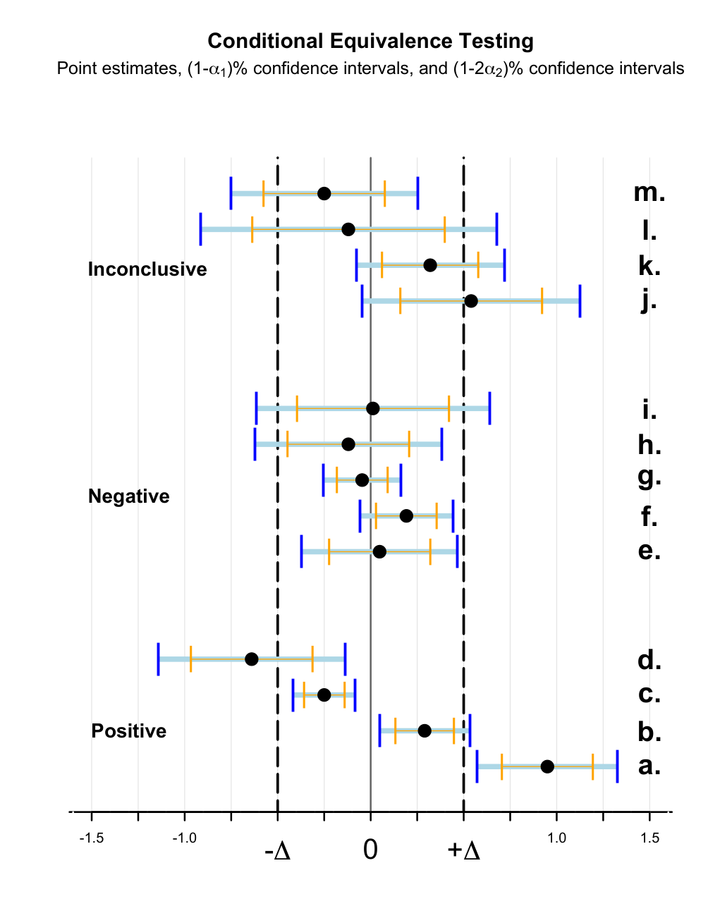
Figure 1 illustrates the three conclusions with their associated confidence intervals. In this figure, we once again consider two-sample testing of normally distributed data as described for box 2.1., with and . Situation “a”, in which the C.I. is entirely outside the equivalence margin is what Guyatt et al. ((1995)) calls a “definitive-positive” result. The lower confidence limit of the parameter is not only larger than zero (the null value, ), implying a “positive” result, but also is above the threshold. Situations “b” and “c”, in which the C.I. excludes zero and the C.I. is within are considered “positive” results but require some additional interpretation. One could describe the effect in these cases as “significant yet not meaningful” or conclude that there is evidence of a significant effect, yet the effect is likely “not minimally important”. A “positive” result such as “d”, with a wider confidence interval, represents a significant, albeit imprecisely estimated, effect. One could conclude that additional studies, with larger sample sizes, are required to determine if the effect is of a meaningful magnitude.
Evidently, in some cases, the three categories are not sufficient on their own for adequate interpretation. For example, without any additional information the “positive” vs. “negative” distinction between cases “b” and “f” is misleading. These two results appear very similar: in both cases a substantial (i.e. greater than -sized) effect can be ruled out. Indeed, positive result “b” appears much more like the negative result “f” than positive result “a”. Additional language and careful attention to the estimated effect size is required for correct interpretation. While case “k” has a similar point estimate to “b” and “f”, the wider C.I. ( is within C.I.) means that one cannot rule out the possibility of a meaningful effect, and so it is rightly categorized as “inconclusive”.
It may be argued that CET is simply a recalibration of the standard confidence interval, like converting Fahrenheit to Celsius. This is valid commentary and in response, it should be noted that our suggestion to adopt CET (in the place of standard confidence intervals) is not unlike that of Gardner & Altman ((1986)) who suggest that confidence intervals should replace -values; see also Cumming ((2008)) and Reichardt & Gollob ((2016)). One advantage of CET over confidence intervals is that it may improve the interpretation of null results, see Parkhurst ((2001)) and Hauck & Anderson ((1986)). By clearly distinguishing between what is a negative versus an inconclusive result, CET serves to simplify the long “series of searching questions” necessary to evaluate a “failed outcome” (Pocock & Stone, (2016)). However, as can be seen with the examples of Figure 1, the use of CET should not rule the complementary use of confidence intervals. Indeed, the best interpretation of a result will be when using both tools together.

As Dienes & Mclatchie ((2017)) clearly explain, with standard NHST, one is unable to make the “three-way distinction” between the positive, inconclusive and negative (“evidence for ”, “no evidence to speak of”, and “evidence for ”). Figure 2 shows the distribution of standard two-tailed -values under NHST and corresponding values under CET for three different sample sizes. These are the result of two-sample testing of normally distributed data as described for box 2.1, with .
Under the standard null () with NHST, one is just as likely to obtain a large -value as one is to obtain a small -value. Under the standard null with CET, a small value (a large value) will indicate evidence in favour of equivalence given sufficient data. In Figure 2, note that the blue points that fall below the threshold in the upper panels (NHST) remain unchanged in the lower panels (CET). However, blue points that fall above the threshold in the upper panels (NHST) are no longer present in the lower panels (CET). They have been replaced by black points () which, if near the top, suggest evidence in favour of equivalence. This treatment of the larger -values is more conducive to the interpretation of null results bringing to mind the thoughts of Amrhein et al. ((2017)) who write “[a]s long as we treat our larger -values as unwanted children, they will continue disappearing in our file drawers, causing publication bias, which has been identified as the possibly most prevalent threat to reliability and replicability.”
2.1 Defining the equivalence margin
As with standard equivalence and non-inferiority testing, defining the equivalence margin will be one of the “most difficult issues” for CET (Hung et al., (2005)). If the margin is too large, then a claim of equivalence is meaningless. If the margin is too small, then the probability of declaring equivalence, will be substantially reduced; see Wiens ((2002)). As stated earlier, the margin is ideally chosen as a boundary to exclude ‘minimum clinically meaningful differences’ (Kaul & Diamond, (2006); Greene et al., (2008)). However, “clinically meaningful” effects are difficult to define, and there is generally no clear consensus among stakeholders, Keefe et al. ((2013)). Furthermore, previously agreed-upon meaningful differences may be difficult to ascertain as they are rarely specified in protocols and published results (Djulbegovic et al., (2011)).
In some fields, there are some generally accepted norms. For example, in bioavailability studies, equivalence is routinely defined (and listed by regulatory authorities) as a difference of less than 20%. In oncology trials, a small effect size has been defined as odds ratio or hazard ratio of 1.3 or less, Bedard et al. ((2007)). In ecology, a proposed equivalence region for trends in population size (the log-linear population regression slope) is , Dixon & Pechmann ((2005)).
In cases when a specified equivalence margin may not be as clear-cut, less conventional options have been put forth. Hauck & Anderson ((1986)) propose the concept of using an “equivalence curve” that illustrates results for a range of possibilities. Meyners ((2007)) proposes to use the least equivalent allowable difference (LEAD), the largest possible value of for which one can claim equivalence. The public would then be left to draw their own conclusions from the data and whether they believe the LEAD- is a reasonable standard for equivalence. This would no doubt lead to a discussion about which effect sizes are too small to be worthwhile for a given treatment, and advance researchers towards a specific standard.
One important choice a researcher must make in defining the equivalence margin is whether the margin should be defined on a raw or standardized scale. Lakens ((2017)) discusses the pros and cons of each option. For example, if there is no rationale for any standard margin in our two-sample normal case, taking equivalence to be a difference within half the estimated standard deviation, i.e. defining , with pre-specified =0.5 seems reasonable. Note, that the probability of obtaining a negative result may be zero (or negligible) for certain combinations of values of , , , and . For example, with , , and , for all (with ). As such, must be chosen with additional practical considerations (see additional details in 2.2). For binary and time-to-event outcomes, there is an even greater number of different ways one can define the margin (e.g. in terms of relative risk vs. odds ratio). For discussions on this, see Ng ((2008)), da Silva et al. ((2009)), Tsou et al. ((2007)) and Barker et al. ((2001)).
It is important to note that, while it may be ideal to specify the margin prior to collecting data, setting the margin afterwards will not lead to any type I error inflation (i.e. one will not erroneously reject with probability greater than ). For the same reason that a 95% C.I. is just as valid as a 85% C.I., but must be interpreted differently, CET is valid regardless of whether the margin is specified (on a raw, or a standardized scale by defining ) before or after data are obtained. However, the conclusion made will clearly depend upon the margin chosen, and for any non-positive result, it is always be possible to choose a specific margin (or specific value for ) which leads to a negative conclusion (see Figure 1). Since the choice of margin is often a difficult one in the best of circumstances, a retrospective choice is not ideal as there will be ample room for bias in one’s choice, regardless of how well intentioned one may be. For this reason, for equivalence and non-inferiority RCTs, it is generally expected that margins are to be pre-specified (Piaggio et al., (2006)).
2.2 Operating characteristics and sample size calculations
What follows is a brief overview of how to calculate the probabilities of obtaining each of the three conclusions (positive, negative, and inconclusive) as listed in our CET procedure above for two-sample testing of normal data with equal variance (box 2.1). More in-depth related work includes Shieh ((2016)) who establishes exact power calculations for TOST for equivalence of normally distributed data and da Silva et al. ((2009)) who review power and sample size calculations for equivalence testing of binary and time-to-event outcomes.
As before, let the true population mean difference be and the true population variance equal . Let and . Figure 3 illustrates how each of the three conclusions can be reached based on the values of and obtained from the data. For this plot, (with ), , and . The black lettered points correspond to the scenarios of Figure 1. The interior diamond, , (with corners located at [0,0], ) covers the values for which a negative conclusion is obtained. A positive conclusion corresponds to when is large and is relatively small. Note how and impact the conclusion. If the equivalence margin is sufficiently wide, one will have approach zero as approaches zero. Indeed, the ratio of determines, to a large extent, the probability of a negative result. If the equivalence margin is sufficiently narrow and the variance relatively large (i.e. is very small), one will have .
Let us assume for simplicity that . Then, the sampling distributions of the sample mean and sample variance are well established: and . Therefore, given fixed values for and , we can calculate the probability of obtaining a positive result, . In Figure 3, equals the probability of and falling into either the left or right “positive” corners and is calculated (as in a usual power calculation for NHST):
| (1) |
where is the cdf of the non-central distribution with degrees of freedom and non-centrality parameter .
One can calculate the probability of obtaining a negative result, , as the probability of and falling into the “negative” diamond, . Since and are independent statistics, we can write their joint density as the product of a normal probability density function, , and a chi-squared probability density function, . However, the resulting double integral will remain difficult to evaluate algebraically over the boundary, . Therefore, the probability is best approximated numerically, for example, by Monte Carlo integration, as follows:
where is the normal cdf and Monte Carlo draws from a chi-squared distribution provide , with for . The left and right-hand boundaries of the diamond-shaped “negative region”, are defined by and .
Defining the boundary with and allows for three distinct cases as seen in Figure 3:
(1) , in which case ;
(2) , in which case and ; and
(3) , in which case and .
When the equivalence boundaries are defined as a function of (e.g. ), the calculations are somewhat different; Figure 4 illustrates. In particular, a negative conclusion requires: (i.e. the % C.I. is entirely within ). As such, for a given sample size, it will only be possible to obtain a negative result if . Likewise, an inconclusive result will only be possible if .
In order to determine an appropriate sample size for CET, one must replace with an a-priori estimate, , the “anticipated effect size”, and replace with an a-priori estimate, , the “anticipated variance”. Then one might be interested in calculating six values: the probabilities of obtaining each of the three possible results (positive, negative and inconclusive) under two hypothetical scenarios, (1) where , and (2) where equal to , the value expected given results in the literature. One might also be interested in a hybrid approach whereby one specifies a composite null and alternative distribution. Since the objective of any study should be to obtain a conclusive result, sample size could also be calculated with the objective to maximize the likelihood of success, i.e. to minimize .
The quantity:
| (2) |
represents the probability of a “successful” study under the assumption that the null () and alternative (with specified ) are equally likely. (Note that both false positive-, and false negative- studies in this equation are considered “successful”.) This weighted average could be considered a simple version of what is known as “assurance” (O’Hagan et al., (2005)). Figure 5 shows how consideration of as the criteria for determining sample size attenuates the effect of on the required sample size. Suppose one calculates that the required sample size is based on the desire for 90% statistical power and the belief that = 1 and =0.205, with as before. This corresponds to a probability of success for =0.1025 (=). If the true variance is slightly larger than anticipated, =1.25, and the difference in means smaller, =0.123, the actual sample size needed for 90% power is in fact =3,476, while the actual sample size needed for is =1,770. On the other hand, if the true variance is slightly smaller than anticipated, and the difference in means greater, =0.33, the actual sample size needed for 90% power is only =288, while the actual sample size needed for =61% is =638. It follows that, if one has little certainty in and , calculating the required sample size with consideration of may be less risky.
For related work on statistical power, see Shao et al. ((2008)) who propose a hybrid Bayesian-frequentist approach to evaluate power for testing both superiority and non-inferiority. Jia & Lynn ((2015)) discuss a related sample size planning approach that considers both statistical significance and clinical significance. Finally, Jiroutek et al. ((2003)) advocate that, rather than calculate statistical power (the probability of rejecting should the alternative be true), one should calculate the probability that the width of a confidence interval is less than a fixed constant and the null hypothesis is rejected, given that the confidence interval contains the true parameter.
3 A comparison with Bayesian testing
Recently, Bayesian statistics have been advocated for, as a “possible solution to publication bias” (Konijn et al., (2015)). In particular, there have been many Bayesian testing schemes proposed in the psychology literature; see the discussion of Mulder & Wagenmakers ((2016)) and, for an accessible overview of the “Bayesian -test”, see Gönen ((2010)). What’s more, publication policies based on Bayesian testing schemes are currently in use by a small number of journals and are the preferred approach for some (e.g. Dienes & Mclatchie ((2017))). In response to these developments, we will compare, with regards to their operating characteristics, CET and a Bayesian testing scheme. This brings to mind Dienes ((2014)) who compares testing with Bayes Factors (BF) to testing with “interval methods” and notes that with interval methods, a study result is a “reflection of the data”, whereas with BFs the result reflects the “evidence of one theory over another”. What follows is a brief overview of one Bayesian scheme and an investigation of how it compares to CET.
The Bayes Factor is a valuable tool for determining the degree of evidence for the absence of a treatment effect, see most recently Hoekstra et al. ((2017)). Consider, for the two-sample testing of normally distributed data (as described for box 2.1), a Bayes Factor testing scheme in which we take the JZS (Jeffreys-Zellner-Siow) prior for the alternative hypothesis, see Rouder et al. ((2009)). Note that, for the Bayes Factor, the null hypothesis, , corresponds to ; and the alternative, , corresponds to .
The JZS testing scheme involves placing a normal prior on , , and for the hyper-parameter , placing an inverse chi-squared prior, . Integrating out shows that this is equivalent to having a Cauchy prior, . The JZS prior is recommended as a reasonable “objective prior” to be used in a Bayesian alternative to the common frequentist -test (Rouder et al., (2009)). We can write the JZS Bayes Factor in terms of the standard -statistic, , with , as follows:
| (3) |
Figure 6 -left panel shows how the JZS Bayes Factor changes with sample size for four different values of the observed difference in means, ; the observed variance remains constant at . When the observed mean difference is exactly 0, the BF increases logarithmically with . For small to moderate , the BF supports the null for small values of but, as becomes larger, yields less support for the null and eventually favours the alternative. The horizontal lines mark the 3:1 and 1/3 thresholds (“moderate evidence”) as well as the 10:1 and 1/10 thresholds (“strong evidence”).
Figure 6 -right panel shows -values for the same four values of , constant , and the equivalence margin of . The lines suggest that CET possesses similar “ideal behaviour” (Rouder et al., (2009)) as is observed with the BF. When the observed mean difference is exactly zero, CET provides increasing evidence in favour of equivalence with increasing . For small to moderate , CET supports the null at first and then, as becomes larger, at a certain point favours the alternative. The sharp change-point represents border cases. Consider case “f” in Figure 1: if increased, the confidence intervals would shrink and at a certain point, the C.I. would be exclude 0 (similar to case “b”). At that point, the result abruptly changes from “negative” to “positive”. While this abrupt change may appear odd at first, it may in fact be more desirable than the smooth transition of the BF. Consider for example when . Then for between 112 and 496, the BF will be strictly above 1/3 and strictly below 3, and as such the result, by BF, is inconclusive. In contrast, for the same range in sample size, will be either above 0.90 or below 0.05. As such, with and , a conclusive result is obtained. While careful interpretation is required (e.g. “the effect is significant yet not of a meaningful magnitude”), this may be preferable in some settings to the BF’s inconclusive result.
We can also consider the posterior probability of (i.e. ) equal to (when the prior probabilities and are equal), plotted in Figure 6 -middle panel. The similarities and differences between -values and posterior probabilities have been widely discussed; see Berger & Delampady ((1987)) and more recently Greenland & Poole ((2013)) and Marsman & Wagenmakers ((2017)). Figure 5 suggests that the JZS-BF and CET testing may often result in similar conclusions. We investigate this further by means of a simple simulation study.
3.1 Simulation Study
We conducted a small simulation study to compare the operating characteristics of testing with the JZS-BF relative to with the CET approach. CET conclusions were based on setting , =0.05 and =0.10. JZS BF conclusions were based on a threshold of 3 or greater for evidence in favour of the a negative result and less than 1/3 for evidence in favour of a positive result. BFs in the 1/3 - 3 range correspond to an inconclusive result. A threshold of 3:1 can be considered “substantial evidence” (Wagenmakers et al., (2011)). Note that one advantage of Bayesian methods, is that sample sizes need not be determined in advance; see Rouder ((2014)). Schönbrodt & Wagenmakers ((2016)) list three ways one might design sample size for a study using the BF for testing. For the simulation study here we examine only the “fixed- design”.
For a range of (= 0, 0.07, 0.09, 0.13, 0.18, 0.25, 0.35, 0.48, 0.67) and 14 different sample sizes ( ranging from 10 to 5,000, with ) we simulated normally distributed two-sample datasets (with ). For each dataset, we obtained CET -values, JZS BFs and declared the result to be positive, negative or inconclusive accordingly. Results are presented in Figure 7, based on 5,000 distinct simulated datasets per scenario.
Several findings merit comment:
- •
In this simulation study, the JZS-BF admits a very low frequentist type I error, recorded at most , for a sample size of . As the sample size increases, the frequentist type I error diminishes to a negligible level.
- •
The JZS-BF requires less data to reach a negative conclusion than the CET. However, with moderate to large sample sizes (=100 to 5,000) and small true mean differences ( 0 to 0.25), both methods are approximately equally likely to deliver a negative conclusion.
- •
While the JZS-BF requires less data to reach a conclusion when the true mean difference is small ( 0 to 0.25) (see how solid black curve drops more rapidly than the dashed grey line), there are scenarios in which larger sample sizes will surprisingly reduce the likelihood of obtaining a conclusive result (see how the solid black curve drops abruptly then rises slightly as increases for 0.07, 0.09, 0.13, and 0.18.)
- •
The JZS-BF is always less likely to deliver a positive conclusion (see how dashed blue line is always higher than solid blue line). In the scenarios like those considered, JZS-BF may require larger sample sizes for reaching a positive conclusion and may be considered “less powerful” in a traditional frequentist sense.

The results of the simulation study suggest that, in many ways, the JZS-BF and CET operate very similarly. Think of JZS-BF and CET as two pragmatically similar, yet philosophically different, tools for making “trichotomous significance-testing decisions”. Both tools will often result in the same outcome, given the same data.
4 A CET publication policy
Many researchers have put forth ideas for new publication policies aimed at addressing the issue of publication bias. There is a wide range of opinions on how to incorporate more null results into the published literature. Consider just a few interesting ideas. In an editorial titled “Journals Should Publish All Null Results and Should Sparingly Publish Positive Results.”, Ioannidis ((2006)) writes: “Null results should be published promptly in print in short versions, with more extensive details in web-based files. Positive results should be published equally promptly, but only on the web, pending independent replication; once refuted, the original article and the refutation could be printed as a single nice null report; the rare validated findings should appear in print with full details.” Another suggestion is that of Shields ((2000)) who advocates accepting null papers in a special section of a journal, under the category of “Null Results in Brief”. The null papers in this section, would provide only a brief summary of the methods and results of the studies. With regards to power, Shields ((2000)) states that: “For the [null] paper to be considered for publication, there must be sufficient statistical power to test the a-priori hypothesis. For example, the authors should state the level of power to detect an odds ratio of 2.0 with the current sample size.” Dirnagl et al. ((2010)) makes a similar suggestion with the note that “the quality of the data submitted to our Negative Results section must meet the same rigorous standards that our journal applies to all other submissions. In fact, it may be said that the standards must even exceed those applied currently, as type II error (false negatives) considerations need to be included.”

Certainly one of the most exciting proposals of late is that of Registered Reports (RR). RR is one of many proposed “two-step” manuscript review schemes in which acceptance for publication is granted prior to obtaining the results, see e.g. Walster & Cleary ((1970)), Lawlor ((2007)) as well as more recently Mell & Zietman ((2014)) and Smulders ((2013)). Figure 8 illustrates the RR procedure and Chambers et al. ((2014)) provide an in-depth explanation answering a number of frequently asked questions. The RR policy has two central components: (1) pre-registration and (2) the “RR commitment to publish”.
Pre-registration can be extremely beneficial as it reduces “researcher degrees of freedom” (Simmons et al., (2011)) and prevents, to a large degree, many questionable research practices including data-dredging (Berry, (1990)), the post-hoc fabrication of hypotheses, (“HARKing”) (Kerr, (1998)), and -hacking (Gelman & Loken, (2013)). However, on its own, pre-registration does little to prevent publication bias. This is simply because pre-registration: (a1) cannot prevent authors from disregarding negative results (Song et al., (2014)); (a2) does nothing to prevent reviewers and editors from rejecting studies for lack of significance; and (a3) does not guarantee that peer reviewers consider compliance with the pre-registered analysis plan (van Lent et al., (2015); Mathieu et al., (2013); Chan et al., (2008)).33 3 This paragraph based in part on the post from “ff524” at https://academia.stackexchange.com/questions/74711/why-isnt-pre-registration-required-for-all-experiments.
Consider the field of medicine as a case study. For over a decade, pre-registration of clinical trials has been required by major journals as a prerequisite for publication. Despite this heralded policy change, selective outcome reporting remains ever prevalent, (Ramsey & Scoggins, (2008); Mathieu et al., (2009); Ross et al., (2009); Huić et al., (2011)). (This being said, new 2017/2018 guidelines for the clinicaltrial.gov registry show much promise in addressing a1, a2, and a3; see Zarin et al. ((2016)).)
In order to prevent publication bias, RR complements pre-registration with a “commitment to publish”. In practice this consists of an “in principle acceptance” policy along with the policy of publishing “withdrawn registration" (WR) studies. In order to counter authors who may simply shelve negative results following pre-registration (a1), RR journals commit to publishing the abstracts of all withdrawn studies as WR papers. By guaranteeing that, should a study follow its pre-registered protocol, it will be accepted for publication (“in principle acceptance”), RR prevents reviewers and editors from rejecting a study based on the results (a2). Finally, RR requires that a study is in strict compliance with the pre-registered protocol if it is to be published (a3). In order to keep a RR journal relevant (not simply full of inconclusive studies), RR requires, as part of registration, a researcher commit to a sample size large enough of achieve 90% (in some cases 80%) statistical power. In a small number of RR journals, a Bayesian alternative option is offered. Instead of committing to a specific sample size, researchers commit to achieving a certain BF.
The policy we put forth here is not meant to be an alternative to the “pre-registration” component of RR. Its benefits are clear, and in our view is most often “worth the effort” (Wager & Williams, (2013)). If implemented properly, pre-registration should not “stifle exploratory work” (Gelman, (2013)). Instead, what follows is an alternative to the second “commitment to publish” component.
4.1 Outline of a CET-based publication policy

Figure 9 illustrates the steps of our proposed policy. What follows is a general outline.
Registration- In the first stage of a CET-based policy, before any data are collected, a researcher will register the intent to conduct a study with a journal’s editor. As in a RR policy, this registration process will detail the motivations and merits of the study and list the defined outcomes, the various hypotheses to be tested, and the proposed methods for analysis. Unlike in the RR policy, the registration will not require a sample size calculation showing a specific level of statistical power. Instead, the researcher will define an equivalence margin for each hypothesis test to be carried out. For example if a researcher intends to fit a linear regression model with five explanatory variables, a margin should be defined for each of the five variables. A target sample size should be stated, but need not be justified with regards to power considerations. The researcher will also need to note if there are plans for any sample size reassessments, interim and/or futility analyses.
Editorial and Peer Review- If the merits of the study satisfy the editorial board, the registration study plan will then be sent to reviewers to assess whether the methods for analysis are adequate and whether the equivalence margins are sufficiently narrow. Once the peer reviewers are satisfied (possibly after revisions to the registration plan), the journal will then agree, in principle, to accept the study for eventual publication, on condition that either a positive or a negative result is obtained.
Data collection- Armed with this “in principle acceptance”, the researcher will then collect data in an effort to meet the established sample size target. Once the data are collected and analyses complete, the study will be published if and only if either a positive or negative result is obtained as defined by the pre-specified equivalence margins. Inconclusive results will not generally be published thus protecting a journal from becoming a “dumping ground” for failed studies. In very rare circumstances, however, it may be determined that an inconclusive study offers a substantial contribution to the field and should therefore be considered for publication. As is required practice for good reporting, any failure to meet the target sample size should be stated clearly, along with a discussion of the reasons for failure and the consequences with regards to the interpretation of results; see Toerien et al. ((2009)).
This proposed policy is most similar to the RR Bayesian option outlined in Section 3. Journals only commit (“in principle acceptance”) to publish conclusive studies (small -value/ BF above or below a certain threshold) and no a-priori sample size requirements are forced upon a researcher. As noted in Section 3, we expect that the conclusions obtained under either policy will often be the same. The CET-based policy therefore represents a frequentist alternative to the RR-BF policy.
A journal may wish to require stricter or weaker requirements for publication of results and this can be done by setting thresholds for and accordingly, (e.g. stricter thresholds: ; weaker thresholds: ). Also, note that a -value may be used in one way for the interpretation of results and another way to inform publication decisions. Recently, a large number of researchers (Benjamin et al., (2017)) have publically suggested that the threshold for defining “statistical significance” be changed from to . However, they are careful to emphasize that while this stricter threshold should change the description and interpretation of results, it should not change “standards for policy action nor standards for publication”.
“Gaming the system”- When evaluating a new publication policy one should always ask how (and how easily) a researcher could -unintentionally or not- “game the system”. For the CET-policy as described above, we see one rather obvious strategy.
Consider the following, admittedly extreme, example. A researcher submits 20 different study protocols for pre-registration each with very small sample size targets (e.g. ). Suspend any disbelief, and suppose these studies all have good merit, are all well written, and are all well designed (besides being severely underpowered), and are therefore all granted in principle acceptance. Then, in the event that the null is true (i.e. ) for all 20 studies (and with ), it is expected that at least one study out of the 20 will obtain a positive result and thus be published. This is publication bias at its worst.
In order to discourage this unfortunate practice, we suggest making a researcher’s history of pre-registered studies available to the public. The researcher “gaming the system” in this way will still score his one “type I error” publication, but it will also be known to the public that in 19 other experiments, research was unsuccessful and valuable resources were essentially wasted. With digital identifiers such as ORCID (Haak et al., (2012)), it should be straightforward to maintain a track record across journals and disciplines of the number of successful and unsuccessful studies for each researcher/laboratory. However, while potentially beneficial, we do not anticipate this type of action being necessary. With the CET-policy, it is no longer in a researcher’s interest to “game the system”.
Consider once again, our extreme example. The strategy has an approximately 64% chance of obtaining at least one publication at a cost of 20 submissions and a total of observations. If the goal is to maximize the probability of being published (Charlton & Andras, (2006)), then it is far more efficient to submit a single study with , in which case there is an approximately 98% chance of obtaining a publication (i.e. with , ; 92% chance with , ).
5 Conclusion
Publication bias has been recognized as a serious problem for several decades now (Rosenthal, (1979)). Yet, in many fields, it is only getting worse (Pautasso, (2010)). An investigation by Kühberger et al. ((2014)) concludes that the “entire field of psychology” is now tainted by “pervasive publication bias”.
There remains substantial disagreement on the merits of pre-registration and result-blind peer-review (see e.g. Coffman & Niederle ((2015)); de Winter & Happee ((2013)); van Assen et al. ((2014))). Yet, all can agree that innovative publication policy prescriptions can be part of the solution to the “reproducibility crisis”. While some call for dropping -values and strict thresholds of evidence altogether, we believe that it is not worthwhile to fight “the temptation to discretize continuous evidence and to declare victory” (Gelman & Carlin, (2017)). Instead, the research community should embrace this “temptation” and work with it to achieve desirable outcomes. Indeed, one way to address the “practical difficulties that reviewers face with null results” (Findley et al., (2016)) is to further discretize continuous evidence by means of equivalence testing and we submit that CET can be an effective tool for distinguishing those “high-quality null results” (Shields et al., (2009)) worthwhile of publication.
Recently, a number of influential researchers (McShane et al., (2017)) have argued that to address low reliability, scientists, reviewers and regulators should “abandon statistical significance”. (Somewhat ironically, in some fields, such as reinforcement learning, the currently proposed solution is just the opposite: the adoption of “significance metrics and tighter standardization of experimental reporting” (Henderson et al., (2017)).) We recognize that current publication policies, in which evidence is dichotomized (without any “ontological basis”) may be highly unsatisfactory. However, one benefit to adopting distinct categories based on clearly defined thresholds (as in the CET-policy) is that one can assess, in a systematic way, the state of published research (in terms of reliability, power, reproducibility, etc.). While using a “more holistic view of the evidence” to inform publication decisions may (or may not?) prove effective, ‘meta-research’ under such a paradigm is clearly less feasible. As such, the question of effectiveness may perhaps never be adequately answered.
Bayesian approaches offer many benefits. However, we see three main drawbacks. First, adopting Bayesian testing requires a substantial paradigm shift. Since the interpretation of findings deemed significant by traditional NHST may differ with Bayes, some will no doubt be reluctant to accept the shift. With CET, the traditional usage and interpretation of the -value remains unchanged, except in circumstances when one fails to reject the null. As such, CET does not change the interpretation of findings already established as significant. Indeed, CET simply “extend[s] the arsenal of confirmatory methods rooted in the frequentist paradigm of inference” (Wellek, (2017)). Second, as we observed in our simulation study, Bayesian testing is potentially less powerful than NHST (in the traditional frequentist sense, with a fixed sample size design) and as such could require substantially larger sample sizes. Finally, we share the concern of Morey & Rouder ((2011)) who write that Bayesian testing “provides no means of assessing whether rejections of the nil [null] are due to trivial or unimportant effect sizes or are due to more substantial effect sizes.” For these reasons, we believe CET should be welcomed by any “pragmatic Bayesian” (Kass et al., (2006)).
There are many potential areas for further research. Determining whether and/or and/or should be chosen with consideration of the sample size is important and not trivial; related work includes Pérez & Pericchi ((2014)) who put forward a “Bayes/non-Bayes compromise” in which the -level of a confidence interval changes with . Issues which have proven problematic for standard equivalence testing must also be addressed for CET. These include multiplicity control (Lauzon & Caffo, (2009)) and potential problems with interpretation (Aberegg et al., (2017)). It would also be worthwhile considering whether CET is appropriate for testing for baseline balance, Senn ((1994)). Finally, the impact of a CET policy on meta-analysis should be examined, Hedges ((1992)) (i.e. how should one account for the exclusion of inconclusive results in the published literature when deriving estimates in a meta-analysis?).
The publication policy outlined here should be welcomed by journal editors, researchers and all those who wish to see more reliable science. Research journals which wish to remain relevant and gain a high impact factor should welcome the CET-policy as it offers a mechanism for excluding inconclusive results while providing a space for potentially impactful negative studies. Embracing equivalence testing is an effective way to make publishing null results “more attractive” (O’Hara, (2011)). Researchers should be pleased with a policy that provides “in principle acceptance” and does not insist on specific sample size requirements that may not be feasible or desirable.
The requirement to specify an equivalence margin prior to collecting data will have the additional benefit of forcing researchers and reviewers to think about what would represent a meaningful effect size before embarking on a given study. While there will no doubt be pressure on researchers to “-hack” in order to meet either the the or threshold, this can be discouraged by insisting that an analysis strictly follows the pre-registered analysis plan. Adopting strict thresholds for significance can also act as a deterrent. Finally, we believe that the CET-policy will improve the reliability of published science by not only allowing for more negative research to be published, but by modifying the incentive structure driving research (Nosek et al., (2012)).
Using an optimality model, Higginson & Munafò ((2016)) conclude that, given current incentives, the rational strategy of a scientist is to “focus almost all of their research effort on underpowered exploratory work [… and] carry out lots of underpowered small studies to maximize their number of publications, even though this means around half will be false positives.” This result is in line with the views of many (e.g. Bakker et al. ((2012)), Button et al. ((2013)) and Gervais et al. ((2015))), and provides the basis for why statistical power in many fields has not improved (Smaldino & McElreath, (2016)) despite being highlighted as an issue over six decades ago (Cohen, (1962)). A CET-based policy may provide the incentive scientists need to pursue higher statistical power. If CET can change the incentives driving research, the reliability of science will be further improved. More research on this question (i.e. “meta-research”) is needed.
Acknowledgments
We gratefully acknowledge support from Natural Sciences and Engineering Research Council of Canada. We also wish to thank Drs. John Petkau and Will Welsh for their valuable feedback.
References
- [1] Aberegg, S.K., Hersh, A.M. & Samore, M.H. (2017). Empirical consequences of current recommendations for the design and interpretation of noninferiority trials. Journal of General Internal Medicine .
- [2] Altman, D.G. & Bland, J.M. (1995). Statistics notes: Absence of evidence is not evidence of absence. BMJ 311 7003 485.
- [3] Amrhein, V., Korner-Nievergelt, F. & Roth, T. (2017). The earth is flat (p 0.05): Significance thresholds and the crisis of unreplicable research Tech. Rep.. : PeerJ Preprints.
- [4] Aycaguer, L.C.S. & Galbán, P.A. (2013). Explicación del tamaño muestral empleado: una exigencia irracional de las revistas biomédicas. Gaceta Sanitaria 27 1 53–57.
- [5] Bacchetti, P. (2002). Peer review of statistics in medical research: the other problem. BMJ 324 7348 1271–1273.
- [6] Bakker, M., van Dijk, A. & Wicherts, J.M. (2012). The rules of the game called psychological science. Perspectives on Psychological Science 7 6 543–554.
- [7] Barker, L., Rolka, H., Rolka, D. & Brown, C. (2001). Equivalence testing for binomial random variables: which test to use? The American Statistician 55 4 279–287.
- [8] Bedard, P.L., Krzyzanowska, M.K., Pintilie, M. & Tannock, I.F. (2007). Statistical power of negative randomized controlled trials presented at american society for clinical oncology annual meetings. Journal of Clinical Oncology 25 23 3482–3487.
- [9] Benjamin, D.J., Berger, J.O., Johannesson, M., Nosek, B.A., Wagenmakers, E-J., Berk, R.others (2017). Redefine statistical significance. Nature Human Behaviour .
- [10] Berger, J.O. & Delampady, M. (1987). Testing precise hypotheses. Statistical Science 2 3 317-335.
- [11] Berry, A. (1990). Subgroup analyses. Biometrics 46 4 1227–1230.
- [12] Bland, J.M. (2009). The tyranny of power: is there a better way to calculate sample size? BMJ 339 b3985.
- [13] Borm, G.F., den Heijer, M. & Zielhuis, G.A. (2009). Publication bias was not a good reason to discourage trials with low power. Journal of Clinical Epidemiology 62 1 47–53.
- [14] Button, K.S., Ioannidis, J.P., Mokrysz, C., Nosek, B.A., Flint, J., Robinson, E.S. & Munafò, M.R. (2013). Power failure: why small sample size undermines the reliability of neuroscience. Nature Reviews Neuroscience 14 5 365–376.
- [15] Chalmers, I. & Matthews, R. (2006). What are the implications of optimism bias in clinical research? The Lancet 367 9509 449–450.
- [16] Chambers, C.D., Dienes, Z., McIntosh, R.D., Rotshtein, P. & Willmes, K. (2015). Registered reports: realigning incentives in scientific publishing. Cortex 66 A1–A2.
- [17] Chambers, C.D., Feredoes, E., Muthukumaraswamy, S.D. & Etchells, P. (2014). Instead of “playing the game” it is time to change the rules: Registered reports at aims neuroscience and beyond. AIMS Neuroscience 1 1 4–17.
- [18] Chan, A-W., Hróbjartsson, A., Jørgensen, K.J., Gøtzsche, P.C. & Altman, D.G. (2008). Discrepancies in sample size calculations and data analyses reported in randomised trials: comparison of publications with protocols. BMJ 337 a2299.
- [19] Charlton, B.G. & Andras, P. (2006). How should we rate research?: Counting number of publications may be best research performance measure. BMJ 332 7551 1214–1215.
- [20] Chavalarias, D., Wallach, J.D., Li, A.H.T. & Ioannidis, J.P. (2016). Evolution of reporting p-values in the biomedical literature, 1990-2015. JAMA 315 11 1141–1148.
- [21] Chen, J.J., Tsong, Y. & Kang, S-H. (2000). Tests for equivalence or noninferiority between two proportions. Drug Information Journal 34 2 569–578.
- [22] Coffman, L.C. & Niederle, M. (2015). Pre-analysis plans have limited upside, especially where replications are feasible. The Journal of Economic Perspectives 29 3 81–97.
- [23] Cohen, J. (1962). The statistical power of abnormal-social psychological research: a review. The Journal of Abnormal and Social Psychology 65 3 145–153.
- [24] Cumming, G. (2008). Replication and -intervals: -values predict the future only vaguely, but confidence intervals do much better. Perspectives on Psychological Science 3 4 286–300.
- [25] Cumming, G. (2014). The new statistics: Why and how. Psychological Science 25 1 7–29.
- [26] Dannenberg, O., Dette, H. & Munk, A. (1994). An extension of welch’s approximate t-solution to comparative bioequivalence trials. Biometrika 81 1 91–101.
- [27] da Silva, G.T., Logan, B.R. & Klein, J.P. (2009). Methods for equivalence and noninferiority testing. Biology of Blood and Marrow Transplantation 15 1 120–127.
- [28] de Winter, J. & Happee, R. (2013). Why selective publication of statistically significant results can be effective. PLoS One 8 6 e66463.
- [29] Dickersin, K., Min, Y-I. & Meinert, C.L. (1992). Factors influencing publication of research results: follow-up of applications submitted to two institutional review boards. JAMA 267 3 374–378.
- [30] Dienes, Z. (2014). Using Bayes to get the most out of non-significant results. Frontiers in Psychology 5 781.
- [31] Dienes, Z. (2016). How Bayes factors change scientific practice. Journal of Mathematical Psychology 72 78–89.
- [32] Dienes, Z. & Mclatchie, N. (2017). Four reasons to prefer Bayesian analyses over significance testing. Psychonomic Bulletin & Review 1–12.
- [33] Dirnagl, U. et al. (2010). Fighting publication bias: introducing the negative results section. Journal of Cerebral Blood Flow and Metabolism: official journal of the International Society of Cerebral Blood Flow and Metabolism 30 7 1263–1264.
- [34] Dixon, P.M. & Pechmann, J.H. (2005). A statistical test to show negligible trend. Ecology 86 7 1751–1756.
- [35] Djulbegovic, B., Kumar, A., Magazin, A., Schroen, A.T., Soares, H., Hozo, I.Schell, M.J. (2011). Optimism bias leads to inconclusive results - an empirical study. Journal of Clinical Epidemiology 64 6 583–593.
- [36] Doshi, P., Dickersin, K., Healy, D., Vedula, S.S. & Jefferson, T. (2013). Restoring invisible and abandoned trials: a call for people to publish the findings. BMJ 346 f2865.
- [37] Dwan, K., Altman, D.G., Arnaiz, J.A., Bloom, J., Chan, A-W., Cronin, E.others (2008). Systematic review of the empirical evidence of study publication bias and outcome reporting bias. PLoS One 3 8 e3081.
- [38] Etz, A. & Vandekerckhove, J. (2016). A Bayesian perspective on the reproducibility project: Psychology. PLoS One 11 2 e0149794.
- [39] Fanelli, D. (2009). How many scientists fabricate and falsify research? a systematic review and meta-analysis of survey data. PLoS One 4 5 e5738.
- [40] Findley, M.G., Jensen, N.M., Malesky, E.J. & Pepinsky, T.B. (2016). Can results-free review reduce publication bias? the results and implications of a pilot study. Comparative Political Studies 49 13 1667–1703.
- [41] Franco, A., Malhotra, N. & Simonovits, G. (2014). Publication bias in the social sciences: Unlocking the file drawer. Science 345 6203 1502–1505.
- [42] Freedman, L.S. (2008). An analysis of the controversy over classical one-sided tests. Clinical Trials 5 6 635–640.
- [43] Gardner, M.J. & Altman, D.G. (1986). Confidence intervals rather than p-values: estimation rather than hypothesis testing. BMJ (Clin Res Ed) 292 6522 746–750.
- [44] Gelman, A. (20131). Commentary: P-values and statistical practice. Epidemiology 24 1 69–72.
- [45] Gelman, A. (20132). Preregistration of studies and mock reports. Political Analysis 21 1 40–41.
- [46] Gelman, A. & Carlin, J. (2017). Some natural solutions to the -value communication problem and why they won’t work.
- [47] Gelman, A. & Loken, E. (2013). The garden of forking paths: Why multiple comparisons can be a problem, even when there is no “fishing expedition” or “p-hacking” and the research hypothesis was posited ahead of time. Department of Statistics, Columbia University .
- [48] Gervais, W.M., Jewell, J.A., Najle, M.B. & Ng, B.K. (2015). A powerful nudge? presenting calculable consequences of underpowered research shifts incentives toward adequately powered designs. Social Psychological and Personality Science 6 7 847–854.
- [49] Goeman, J.J., Solari, A. & Stijnen, T. (2010). Three-sided hypothesis testing: Simultaneous testing of superiority, equivalence and inferiority. Statistics in Medicine 29 20 2117–2125.
- [50] Gönen, M. (2010). The Bayesian t-test and beyond. Statistical Methods in Molecular Biology 179–199.
- [51] Goodman, S. & Greenland, S. (2007). Assessing the unreliability of the medical literature: a response to ‘why most published research findings are false?’. : Johns Hopkins University, Department of Biostatistics; bepress.
- [52] Greene, C.J., Morland, L.A., Durkalski, V.L. & Frueh, B.C. (2008). Noninferiority and equivalence designs: issues and implications for mental health research. Journal of Traumatic Stress 21 5 433–439.
- [53] Greenland, S. (2012). Nonsignificance plus high power does not imply support for the null over the alternative. Annals of Epidemiology 22 5 364–368.
- [54] Greenland, S. & Poole, C. (2013). Living with p-values: resurrecting a Bayesian perspective on frequentist statistics. Epidemiology 24 1 62–68.
- [55] Greenwald, A.G. (1975). Consequences of prejudice against the null hypothesis. Psychological Bulletin 82 1 1–20.
- [56] Greve, W., Bröder, A. & Erdfelder, E. (2013). Result-blind peer reviews and editorial decisions: A missing pillar of scientific culture. European Psychologist 18 4 286–294.
- [57] Guyatt, G., Jaeschke, R., Heddle, N., Cook, D., Shannon, H. & Walter, S. (1995). Basic statistics for clinicians: 2. interpreting study results: confidence intervals. CMAJ: Canadian Medical Association Journal 152 2 169–173.
- [58] Haak, L.L., Fenner, M., Paglione, L., Pentz, E. & Ratner, H. (2012). Orcid: a system to uniquely identify researchers. Learned Publishing 25 4 259–264.
- [59] Harlow, L.L., Mulaik, S.A. & Steiger, J.H. (2016). What if there were no significance tests?: Classic edition. : Routledge.
- [60] Hartung, J., Cottrell, J.E. & Giffin, J.P. (1983). Absence of evidence is not evidence of absence. Anesthesiology: The Journal of the American Society of Anesthesiologists 58 3 298–299.
- [61] Hauck, W.W. & Anderson, S. (1986). A proposal for interpreting and reporting negative studies. Statistics in Medicine 5 3 203–209.
- [62] Hauschke, D., Steinijans, V. & Diletti, E. (1990). A distribution-free procedure for the statistical analysis of bioequivalence studies. International Journal of Clinical Pharmacology, Therapy, and Toxicology 28 2 72–78.
- [63] Hedges, L.V. (1992). Modeling publication selection effects in meta-analysis. Statistical Science 246–255.
- [64] Henderson, P., Islam, R., Bachman, P., Pineau, J., Precup, D. & Meger, D. (2017). Deep reinforcement learning that matters. arXiv preprint arXiv:1709.06560 .
- [65] Higginson, A.D. & Munafò, M.R. (2016). Current incentives for scientists lead to underpowered studies with erroneous conclusions. PLoS Biology 14 11 e2000995.
- [66] Hoekstra, R., Monden, R., van Ravenzwaaij, D. & Wagenmakers, E-J. (2017). Bayesian reanalysis of null results reported in the New England Journal of Medicine: Strong yet variable evidence for the absence of treatment effects. Manuscript submitted for publication .
- [67] Hoenig, J.M. & Heisey, D.M. (2001). The abuse of power: the pervasive fallacy of power calculations for data analysis. The American Statistician 55 1 19–24.
- [68] Hofmann, M.A. (2016). Null hypothesis significance testing in simulation. In Proceedings of the 2016 winter simulation conference ( 522–533).
- [69] Huić, M., Marušić, M. & Marušić, A. (2011). Completeness and changes in registered data and reporting bias of randomized controlled trials in icmje journals after trial registration policy. PLoS One 6 9 e25258.
- [70] Hung, H., Wang, S-J. & O’Neill, R. (2005). A regulatory perspective on choice of margin and statistical inference issue in non-inferiority trials. Biometrical Journal 47 1 28–36.
- [71] Ioannidis, J.P. (2005). Why most published research findings are false. PLoS Medicine 2 8 e124.
- [72] Ioannidis, J.P. (2006). Journals should publish all null results and should sparingly publish ‘positive’ results. Cancer Epidemiology Biomarkers & Prevention 15 1 186–186.
- [73] Jia, B. & Lynn, H.S. (2015). A sample size planning approach that considers both statistical significance and clinical significance. Trials 16 1 213.
- [74] Jiroutek, M.R., Muller, K.E., Kupper, L.L. & Stewart, P.W. (2003). A new method for choosing sample size for confidence interval–based inferences. Biometrics 59 3 580–590.
- [75] Jonas, K.J. & Cesario, J. (2017). Submission guidelines for authors, comprehensive results in social psychology. www.tandf.co.uk/journals/authors/rrsp-submission-guidelines.pdf .
- [76] Kass, R.E. et al. (2006). Kinds of Bayesians (comment on articles by berger and by goldstein). Bayesian Analysis 1 3 437–440.
- [77] Kaul, S. & Diamond, G.A. (2006). Good enough: a primer on the analysis and interpretation of noninferiority trials. Annals of Internal Medicine 145 1 62–69.
- [78] Keefe, R.S., Kraemer, H.C., Epstein, R.S., Frank, E., Haynes, G., Laughren, T.P.Leon, A.C. (2013). Defining a clinically meaningful effect for the design and interpretation of randomized controlled trials. Innovations in Clinical Neuroscience 10 5-6 Suppl A 4S.
- [79] Kerr, N.L. (1998). Harking: Hypothesizing after the results are known. Personality and Social Psychology Review 2 3 196–217.
- [80] Konijn, E.A., van de Schoot, R., Winter, S.D. & Ferguson, C.J. (2015). Possible solution to publication bias through Bayesian statistics, including proper null hypothesis testing. Communication Methods and Measures 9 4 280–302.
- [81] Koyama, T. & Westfall, P.H. (2005). Decision-theoretic views on simultaneous testing of superiority and noninferiority. Journal of Biopharmaceutical Statistics 15 6 943–955.
- [82] Kruschke, J.K. & Liddell, T.M. (2017). The Bayesian new statistics: Hypothesis testing, estimation, meta-analysis, and power analysis from a Bayesian perspective. Psychonomic Bulletin & Review 1–29.
- [83] Kühberger, A., Fritz, A. & Scherndl, T. (2014). Publication bias in psychology: a diagnosis based on the correlation between effect size and sample size. PLoS One 9 9 e105825.
- [84] Lakens, D. (2017). Equivalence tests: A practical primer for t tests, correlations, and meta-analyses. Social Psychological and Personality Science 1948550617697177.
- [85] Lash, T.L. (2017). The harm done to reproducibility by the culture of null hypothesis significance testing. American Journal of Epidemiology 1–9.
- [86] Lauzon, C. & Caffo, B. (2009). Easy multiplicity control in equivalence testing using two one-sided tests. The American Statistician 63 2 147–154.
- [87] Lawlor, D.A. (2007). Quality in epidemiological research: should we be submitting papers before we have the results and submitting more hypothesis-generating research? : Oxford University Press.
- [88] Lew, M.J. (2013). To p or not to p: On the evidential nature of p-values and their place in scientific inference. arXiv preprint arXiv:1311.0081 .
- [89] Marsman, M. & Wagenmakers, E-J. (2017). Three insights from a Bayesian interpretation of the one-sided p-value. Educational and Psychological Measurement 77 3 529–539.
- [90] Mathieu, S., Boutron, I., Moher, D., Altman, D.G. & Ravaud, P. (2009). Comparison of registered and published primary outcomes in randomized controlled trials. JAMA 302 9 977–984.
- [91] Mathieu, S., Chan, A-W. & Ravaud, P. (2013). Use of trial register information during the peer review process. PLoS One 8 4 e59910.
- [92] Matthews, J.N. (1995). Small clinical trials: are they all bad? Statistics in Medicine 14 2 115–126.
- [93] McShane, B.B., Gal, D., Gelman, A., Robert, C. & Tackett, J.L. (2017). Abandon statistical significance. arXiv preprint arXiv:1709.07588 .
- [94] Mell, L.K. & Zietman, A.L. (2014). Introducing prospective manuscript review to address publication bias. International Journal of Radiation Oncology -Biology Physics 90 4 729–732.
- [95] Meyners, M. (2007). Least equivalent allowable differences in equivalence testing. Food Quality and Preference 18 3 541–547.
- [96] Meyners, M. (2012). Equivalence tests–a review. Food Quality and Preference 26 2 231–245.
- [97] Morey, R.D. & Rouder, J.N. (2011). Bayes factor approaches for testing interval null hypotheses. Psychological Methods 16 4 406–419.
- [98] Mulder, J. & Wagenmakers, E-J. (2016). Editors’ introduction to the special issue ‘Bayes factors for testing hypotheses in psychological research: Practical relevance and new developments’. Journal of Mathematical Psychology 72 1–5.
- [99] Ng, T-H. (2003). Issues of simultaneous tests for noninferiority and superiority. Journal of Biopharmaceutical Statistics 13 4 629–639.
- [100] Ng, T-H. (2008). Noninferiority hypotheses and choice of noninferiority margin. Statistics in Medicine 27 26 5392–5406.
- [101] Nickerson, R.S. (2000). Null hypothesis significance testing: a review of an old and continuing controversy. Psychological Methods 5 2 241–301.
- [102] Nosek, B.A., Ebersole, C.R., DeHaven, A. & Mellor, D. (2017). The preregistration revolution. osf.io/2dxu5
- [103] Nosek, B.A., Spies, J.R. & Motyl, M. (2012). Scientific utopia II. restructuring incentives and practices to promote truth over publishability. Perspectives on Psychological Science 7 6 615–631.
- [104] Ocaña i Rebull, J., Sánchez Olavarría, M.P., Sánchez, A. & Carrasco Jordan, J.L. (2008). On equivalence and bioequivalence testing. Sort 32 2 151–176.
- [105] O’Hagan, A., Stevens, J.W. & Campbell, M.J. (2005). Assurance in clinical trial design. Pharmaceutical Statistics 4 3 187–201.
- [106] O’Hara, B. (2011). Negative results are published. Nature 471 7339 448–449.
- [107] Parkhurst, D.F. (2001). Statistical significance tests: Equivalence and reverse tests should reduce misinterpretation equivalence tests improve the logic of significance testing when demonstrating similarity is important, and reverse tests can help show that failure to reject a null hypothesis does not support that hypothesis. Bioscience 51 12 1051–1057.
- [108] Pautasso, M. (2010). Worsening file-drawer problem in the abstracts of natural, medical and social science databases. Scientometrics 85 1 193–202.
- [109] Pérez, M-E. & Pericchi, L.R. (2014). Changing statistical significance with the amount of information: The adaptive significance level. Statistics & Probability Letters 85 20–24.
- [110] Perlman, M.D., Wu, L. et al. (1999). The emperor’s new tests. Statistical Science 14 4 355–369.
- [111] Piaggio, G., Elbourne, D.R., Altman, D.G., Pocock, S.J., Evans, S.J., Group, C. et al. (2006). Reporting of noninferiority and equivalence randomized trials: an extension of the consort statement. JAMA 295 10 1152–1160.
- [112] Pocock, S.J. & Stone, G.W. (2016). The primary outcome fails -what next? New England Journal of Medicine 375 9 861–870.
- [113] Ramsey, S. & Scoggins, J. (2008). Commentary: practicing on the tip of an information iceberg? evidence of underpublication of registered clinical trials in oncology. The Oncologist 13 9 925–929.
- [114] Reichardt, C.S. & Gollob, H.F. (2016). When confidence intervals should be used instead of statistical tests, and vice versa. : Routledge.
- [115] Reysen, S. (2006). Publication of nonsignificant results: a survey of psychologists’ opinions. Psychological Reports 98 1 169–175.
- [116] Rosenthal, R. (1979). The file drawer problem and tolerance for null results. Psychological Bulletin 86 3 638–641.
- [117] Ross, J.S., Mulvey, G.K., Hines, E.M., Nissen, S.E. & Krumholz, H.M. (2009). Trial publication after registration in clinicaltrials.gov: a cross-sectional analysis. PLoS Medicine 6 9 e1000144.
- [118] Rouder, J.N. (2014). Optional stopping: No problem for Bayesians. Psychonomic Bulletin & Review 21 2 301.
- [119] Rouder, J.N., Speckman, P.L., Sun, D., Morey, R.D. & Iverson, G. (2009). Bayesian t tests for accepting and rejecting the null hypothesis. Psychonomic Bulletin & Review 16 2 225–237.
- [120] Sackett, D.L. & Cook, D.J. (1993). Can we learn anything from small trials? Annals of the New York Academy of Sciences 703 1 25–32.
- [121] Schönbrodt, F.D. & Wagenmakers, E-J. (2016). Bayes factor design analysis: Planning for compelling evidence. Psychonomic Bulletin & Review 1–15.
- [122] Schulz, K.F. & Grimes, D.A. (2005). Sample size calculations in randomised trials: mandatory and mystical. The Lancet 365 9467 1348–1353.
- [123] Senn, S. (1994). Testing for baseline balance in clinical trials. Statistics in Medicine 13 17 1715–1726.
- [124] Shao, Y., Mukhi, V. & Goldberg, J.D. (2008). A hybrid Bayesian-frequentist approach to evaluate clinical trial designs for tests of superiority and non-inferiority. Statistics in Medicine 27 4 504–519.
- [125] Shieh, G. (2016). Exact power and sample size calculations for the two one-sided tests of equivalence. PLoS One 11 9 e0162093.
- [126] Shields, P.G. (2000). Publication bias is a scientific problem with adverse ethical outcomes: the case for a section for null results ( 9). : AACR.
- [127] Shields, P.G., Sellers, T.A. & Rebbeck, T.R. (2009). Null results in brief: meeting a need in changing times. Cancer Epidemiology and Prevention Biomarkers 18 9 2347–2347.
- [128] Simmons, J.P., Nelson, L.D. & Simonsohn, U. (2011). False-positive psychology: Undisclosed flexibility in data collection and analysis allows presenting anything as significant. Psychological Science 22 11 1359–1366.
- [129] Smaldino, P.E. & McElreath, R. (2016). The natural selection of bad science. Royal Society Open Science 3 9 160384.
- [130] Smulders, Y.M. (2013). A two-step manuscript submission process can reduce publication bias. Journal of Clinical Epidemiology 66 9 946–947.
- [131] Song, F., Loke, Y. & Hooper, L. (2014). Why are medical and health-related studies not being published? a systematic review of reasons given by investigators. PLoS One 9 10 e110418.
- [132] Sterling, T.D., Rosenbaum, W.L. & Weinkam, J.J. (1995). Publication decisions revisited: The effect of the outcome of statistical tests on the decision to publish and vice versa. The American Statistician 49 1 108–112.
- [133] Suñé, P., Suñé, J.M. & Montoro, J.B. (2013). Positive outcomes influence the rate and time to publication, but not the impact factor of publications of clinical trial results. PLoS One 8 1 e54583.
- [134] Szucs, D. & Ioannidis, J.P. (2016). When null hypothesis significance testing is unsuitable for research: a reassessment. bioRxiv 095570.
- [135] Toerien, M., Brookes, S.T., Metcalfe, C., De Salis, I., Tomlin, Z., Peters, T.J.Donovan, J.L. (2009). A review of reporting of participant recruitment and retention in rcts in six major journals. Trials 10 1 52.
- [136] Trafimow, D. & Marks, M. (2015). Editorial. Basic and Applied Social Psychology 37 1 1-2. doi:10.1080/01973533.2015.1012991
- [137] Tsou, H-H., Hsiao, C-F., Chow, S-C., Yue, L., Xu, Y. & Lee, S. (2007). Mixed noninferiority margin and statistical tests in active controlled trials. Journal of Biopharmaceutical Statistics 17 2 339–357.
- [138] van Assen, M.A., van Aert, R.C., Nuijten, M.B. & Wicherts, J.M. (2014). Why publishing everything is more effective than selective publishing of statistically significant results. PLoS One 9 1 e84896.
- [139] van Lent, M., IntHout, J. & Out, H.J. (2015). Differences between information in registries and articles did not influence publication acceptance. Journal of Clinical Epidemiology 68 9 1059–1067.
- [140] Vasishth, S. & Gelman, A. (2017). The illusion of power: How the statistical significance filter leads to overconfident expectations of replicability. arXiv preprint arXiv:1702.00556 .
- [141] Wagenmakers, E-J. (2007). A practical solution to the pervasive problems of -values. Psychonomic Bulletin & Review 14 5 779–804.
- [142] Wagenmakers, E-J., Wetzels, R., Borsboom, D. & Van Der Maas, H.L. (2011). Why psychologists must change the way they analyze their data: the case of psi: comment on bem (2011).
- [143] Wager, E. & Williams, P. (2013). “hardly worth the effort” -medical journals’ policies and their editors’ and publishers’ views on trial registration and publication bias: quantitative and qualitative study. BMJ 347 f5248.
- [144] Walker, E. & Nowacki, A.S. (2011). Understanding equivalence and noninferiority testing. Journal of General Internal Medicine 26 2 192–196.
- [145] Walster, G.W. & Cleary, T.A. (1970). A proposal for a new editorial policy in the social sciences. The American Statistician 24 2 16–19.
- [146] Wasserstein, R.L. & Lazar, N.A. (2016). The ASA’s statement on -values: context, process, and purpose. The American Statistician 70 2 129–133.
- [147] Wellek, S. (2010). Testing statistical hypotheses of equivalence and noninferiority. : CRC Press.
- [148] Wellek, S. (2017). A critical evaluation of the current “p-value controversy”. Biometrical Journal .
- [149] Wiens, B.L. (2002). Choosing an equivalence limit for noninferiority or equivalence studies. Controlled Clinical Trials 23 1 2–14.
- [150] Wiens, B.L. & Iglewicz, B. (2000). Design and analysis of three treatment equivalence trials. Controlled Clinical Trials 21 2 127–137.
- [151] Zarin, D.A., Tse, T., Williams, R.J. & Carr, S. (2016). Trial reporting in clinicaltrials.gov -the final rule. New England Journal of Medicine 375 20 1998–2004.
- [152] Zhang, X., Cutter, G. & Belin, T. (2011). Bayesian sample size determination under hypothesis tests. Contemporary Clinical Trials 32 3 393–398.
- [153] Zhao, G. (2016). Considering both statistical and clinical significance. International Journal of Statistics and Probability 5 5 16.
- [154] Zumbo, B.D. & Hubley, A.M. (1998). A note on misconceptions concerning prospective and retrospective power. Journal of the Royal Statistical Society: Series D (The Statistician) 47 2 385–388.