跳到论文正文
W Papers独立论文阅读器 arXiv:1710.01694 论文正文 计算阅读时间 · 0%
引用这篇论文根据当前论文元数据生成,正式投稿前建议核对。


License: arXiv.org perpetual non-exclusive license
arXiv:1710.01694v2 [math.NA] 13 Aug 2018

2018 \vol \fpage \lpage \amssayisi2010 AMS Mathematics Subject Classification: 65L10, 65L11

A hybrid simulation for singularly perturbed system of two-point reaction-diffusion boundary-value problems

Süleyman CENGIZCI1 , Srinivasan NATESAN2, Mehmet Tarık ATAY3
1
Department of Computer Programming
††thanks: Correspondence: suleyman.cengizci@antalya.edu.tr
   Antalya Bilim University    Antalya    Turkey
2Department of Mathematics
   Indian Institute of Technology Guwahati    Guwahati    India
3Department of Mechanical Engineering
   Abdullah Gül University    Kayseri    Turkey

\rec28.07.2018 \acc.201 \finv..201
Abstract

This study concerns with singularly perturbed systems of second-order reaction-diffusion equations in ODE’s. To handle this type of problems, a numerical-asymptotic hybrid method is employed. In this hybrid method, an efficient asymptotic method, the so-called Successive complementary expansion method (SCEM) is applied first and then, a numerical method based on finite differences is proposed to approximate the solution of the corresponding singularly perturbed reaction-diffusion systems. Two illustrative examples are provided to show the efficiency and easy-applicability of the present method with convergence properties.

keywords
Singular perturbation problems; reaction-diffusion equations; asymptotic approximation; boundary layers, SCEM, finite difference method.

1 Introduction

System of differential equations arise in many branches of science such as modelling of electrical networks, mechanical systems, marketing problems, earthquake/tsunami problems, chemotaxis processes, semiconductor physics, etc. Because of the physical importance, many studies were devoted to this area. In [8], system of differential equations are studied in detail and in [4, 24] some numerical treatments are examined. On the other hand, singularly perturbed differential equations that involve positive small perturbation parameter(s) 0<ϵ≪10<\epsilon\ll 1 multiplied with the highest order derivative term are also important concept of applied sciences and it is a well-known fact that standard numerical techniques are often insufficient to handle them. Some application areas may be given as control theory, fluid mechanics, quantum mechanics, combustion theory, signal and image processing, pharmacokinetics, etc. One can find theoretical considerations on singular perturbation problems in [31, 25, 27, 10] and various approximation methods in [26, 16, 17, 5, 20, 3, 29].

The present paper concerns with the approximations of the solution of singularly perturbed systems of reaction-diffusion boundary-value problems (BVPs) that frequently arise in electroanalytical chemistry and population dynamics problems. In recent years various methods were employed to obtain approximations to the solution of this kind of problems. In [2, 11], finite difference methods (FDM) for singularly perturbed convection-diffusion systems, in [18, 19] finite element method (FEM) and in [13, 21, 23, 6] finite difference methods for singularly perturbed reaction-diffusion systems are examined. For singularly perturbed system of reaction-diffusion BVPs, in [22], the authors provided a robust computational technique , whereas in [9], optimal order error estimates are obtained on equidistributed grids.

In this paper, we employ a numerical-asymptotic hybrid method for approximating the solution of singularly perturbed system of two-point boundary-value problems reaction-diffusion type. At the first step, an efficient asymptotic method that is introduced in [28], called Successive Complementary Expansion Method (SCEM), and later a finite difference method given in [7] are applied.

In order to examine the convergence of approximations to the solution of singularly perturbed system of differential equations, we need to define the norm that we will use in the remainder parts of this study. In [14] one can find that the appropriate norm for this examination is the maximum norm that is given by

∥r∥=maxΩ¯|r(x)|, ∥r→∥=maxΩ¯{∥ri∥},\|r\parallel=\underset{\overline{\Omega}}{\max}\left|r\left(x\right)\right|,\text{ }\|\overrightarrow{r}\parallel=\underset{\overline{\Omega}}{\max}\left\{\|r_{i}\parallel\right\},

where r→=(r1,r2,⋯,rn).\overrightarrow{r}=\left(r_{1},r_{2},\cdots,r_{n}\right).

The remainder sections of this paper continue as follows: In Section 2, the continuous problem and its general properties are explained. In section 3, the numerical-asymptotic hybrid method that we employ to solve system of singularly perturbed two-point reaction-diffusion equations is described. In section 4, two illustrative examples are provided to show the implementation of the method and in the last section, we discuss the findings.

2 The continuous problem

In general, a coupled system of singularly perturbed reaction-diffusion ODE’s is given as

{−ε​y1′′​(x)+a11​(x)​y1​(x)+a12​(x)​y2​(x)=f1​(x),−η​y2′′​(x)+a21​(x)​y1​(x)+a22​(x)​y2​(x)=f2​(x),\left\{\begin{array}[]{ll}-\varepsilon y_{1}^{\prime\prime}\left(x\right)+a_{11}\left(x\right)y_{1}\left(x\right)+a_{12}\left(x\right)y_{2}\left(x\right)=f_{1}\left(x\right),\\[6.0pt] -\eta y_{2}^{\prime\prime}\left(x\right)+a_{21}\left(x\right)y_{1}\left(x\right)+a_{22}\left(x\right)y_{2}\left(x\right)=f_{2}\left(x\right),\end{array}\right. (2.1)

with some suitable boundary or initial conditions. The presence of positive small parameters 0<ε≪10<\varepsilon\ll 1 and 0<η≪10<\eta\ll 1 causes rapid changes (boundary layers) near the end-points of the domain Ω¯.\overline{\Omega}. These layer behaviors can be examined in three different cases:

Case 1: 𝟎<ε<η≪𝟏\mathbf{0<\varepsilon<\eta\ll 1} In this case, both components of the solution have boundary layers of width O⁡(η​ln⁡η)O\left(\eta\ln\eta\right) and y1​(x)y_{1}\left(x\right) has an additional sublayer of width O⁡(ε​ln⁡ε)O\left(\varepsilon\ln\varepsilon\right).

Case 2: 𝟎<ε≪𝟏\mathbf{0<\varepsilon\ll 1} and η=𝟏\mathbf{\eta=1} In this case, only the first component of the solution has boundary layers of width O⁡(ε​ln⁡ε)O\left(\varepsilon\ln\varepsilon\right).

Case 3: 𝟎<ε=η≪𝟏\mathbf{0<\varepsilon=\eta\ll 1} In this case, both components of the solution have boundary layers of width O⁡(ε​ln⁡ε)O\left(\varepsilon\ln\varepsilon\right) (or equivalently OPENO⁡(η​ln⁡η))O\left(\eta\ln\eta\right)).

We are interested in Case 2 - Case 3 and in finding y→​(x)∈C2​(Ω¯),\overrightarrow{y}\left(x\right)\in C^{2}\left(\overline{\Omega}\right), such that for all x∈Ω=(0,1)x\in\Omega=\left(0,1\right) and for the problem

{−ε​y1′′​(x)+a11​(x)​y1​(x)+a12​(x)​y2​(x)=f1​(x),−ε​y2′′​(x)+a21​(x)​y1​(x)+a22​(x)​y2​(x)=f2​(x),y1(0)=y1(1)=0,y2(0)=y2(1)=0.\left\{\begin{array}[]{ll}-\varepsilon y_{1}^{\prime\prime}\left(x\right)+a_{11}\left(x\right)y_{1}\left(x\right)+a_{12}\left(x\right)y_{2}\left(x\right)=f_{1}\left(x\right),\\[6.0pt] -\varepsilon y_{2}^{\prime\prime}\left(x\right)+a_{21}\left(x\right)y_{1}\left(x\right)+a_{22}\left(x\right)y_{2}\left(x\right)=f_{2}\left(x\right),\\[6.0pt] y_{1}\left(0\right)=y_{1}\left(1\right)=0,\quad y_{2}\left(0\right)=y_{2}\left(1\right)=0.\end{array}\right. (2.2)

The system of BVPs given in (2.2) can be rewritten in the matrix form as

{Lε​y→​(x)=[−ε​d2d​x200−ε​d2d​x2]​y→​(x)+A⁡(x)​y→​(x)=f→​(x),y→​(0)=[y1​(0),y2​(0)]T,y→​(1)=[y1​(1),y2​(1)]T\left\{\begin{array}[]{ll}L_{\varepsilon}\overrightarrow{y}\left(x\right)=\begin{bmatrix}-\varepsilon\frac{d^{2}}{dx^{2}}&0\\ 0&-\varepsilon\frac{d^{2}}{dx^{2}}\end{bmatrix}\overrightarrow{y}\left(x\right)+A\left(x\right)\overrightarrow{y}\left(x\right)=\overrightarrow{f}\left(x\right),\\[10.0pt] \overrightarrow{y}\left(0\right)=\left[y_{1}\left(0\right),y_{2}\left(0\right)\right]^{T},\quad\overrightarrow{y}\left(1\right)=\left[y_{1}\left(1\right),y_{2}\left(1\right)\right]^{T}\end{array}\right. (2.3)

where A⁡(x)=[a11​(x)a12​(x)a21​(x)a22​(x)]A\left(x\right)=\begin{bmatrix}a_{11}\left(x\right)&a_{12}\left(x\right)\\ a_{21}\left(x\right)&a_{22}\left(x\right)\end{bmatrix} and f→​(x)=[f1​(x)f2​(x)].\overrightarrow{f}\left(x\right)=\begin{bmatrix}f_{1}\left(x\right)\\ f_{2}\left(x\right)\end{bmatrix}. The functions ai​j​(x),a_{ij}\left(x\right), fi​(x)∈C2​(Ω)f_{i}\left(x\right)\in C^{2}\left(\Omega\right) for i,j=1,2.i,j=1,2. Now, we should impose two assumptions on problem (2.3). First one is for strictly diagonally dominance of matrix AA and the second one is to be able to establish maximum principle theorem:

Assumption 1 a11​(x)>|a12​(x)|a_{11}\left(x\right)>\left|a_{12}\left(x\right)\right| and a22​(x)>|a21​(x)|,a_{22}\left(x\right)>\left|a_{21}\left(x\right)\right|, for all x∈Ω¯,x\in\overline{\Omega},

Assumption 2 a12​(x)≤0a_{12}\left(x\right)\leq 0 and a21​(x)≤0,a_{21}\left(x\right)\leq 0, for all x∈Ω¯.x\in\overline{\Omega}.

The proof of the following lemma and the corollary can be seen in the paper [21].

Lemma 2.1

(Maximum Principle) Consider the system of singularly perturbed BVP’s (2.3). If y→​(0)⩾0→,\overrightarrow{y}\left(0\right)\geqslant\overrightarrow{0}, y→​(1)⩾0→\overrightarrow{y}\left(1\right)\geqslant\overrightarrow{0} and Lε​y→​(x)⩾0→L_{\varepsilon}\overrightarrow{y}\left(x\right)\geqslant\overrightarrow{0} for all x∈x\in Ω,\Omega, then y→​(x)⩾0→\overrightarrow{y}\left(x\right)\geqslant\overrightarrow{0}, ∀x∈Ω¯.\forall x\in\overline{\Omega}.

Corollary 2.2

(Stability) If y→​(x)\overrightarrow{y}\left(x\right) is the solution of (2.3), then the stability bound inequality

‖y→​(x)‖≤1δ​‖f→‖+‖y→​(0)‖+‖y→​(1)‖\|\overrightarrow{y}\left(x\right)\|\leq\frac{1}{\delta}\|\overrightarrow{f}\|+\|\overrightarrow{y}\left(0\right)\|+\|\overrightarrow{y}\left(1\right)\|

holds, where δ=minΩ¯​{a11​(x)+a12​(x),a21​(x)+a22​(x)}.\delta=\underset{\overline{\Omega}}{\min}\left\{a_{11}\left(x\right)+a_{12}\left(x\right),a_{21}\left(x\right)+a_{22}\left(x\right)\right\}.

Under these above-mentioned assumptions and conditions, the hybrid method can be given as in the next section.

3 The hybrid method

In this section, we first give a short overview of asymptotic approximations and then explain the hybrid method by which we obtain highly accurate approximations to the systems of singularly perturbed differential equations.

Let EE be a set of all real-valued functions that depend on ε,\varepsilon, strictly positive and continuous in (0,ε0](0,\varepsilon_{0}] and such that limε→0δ⁡(ε)\displaystyle\lim_{\varepsilon\rightarrow 0}\delta(\varepsilon) exists and for each δ1​(ε)\delta_{1}\left(\varepsilon\right),δ2​(ε)∈E\delta_{2}\left(\varepsilon\right)\in E, δ1​(ε)​δ2​(ε)∈E\delta_{1}\left(\varepsilon\right)\delta_{2}\left(\varepsilon\right)\in E holds. A function δi​(ε)\delta_{i}(\varepsilon) that satisfies these conditions are called order function. Given two functions ϕ⁡(x,ε)\phi(x,\varepsilon) and ϕa​(x,ε)\phi_{a}(x,\varepsilon) defined in a domain Ω¯\overline{\Omega} are asymptotically identical to order δ⁡(ε)\delta\left(\varepsilon\right) if their difference is asymptotically smaller than δ⁡(ε)\delta\left(\varepsilon\right), where δ⁡(ε)\delta\left(\varepsilon\right) is an order function, that is,

ϕ⁡(x,ε)−ϕa​(x,ε)=o⁡(δ⁡(ε))\phi(x,\varepsilon)-\phi_{a}(x,\varepsilon)=o(\delta(\varepsilon)) (3.1)

where ε\varepsilon is the small parameter arising from the physical problem under consideration. The function ϕa​(x,ε)\phi_{a}(x,\varepsilon) is named as asymptotic approximation of the function ϕ⁡(x,ε).\phi(x,\varepsilon). Asymptotic approximations in general form defined by

ϕa​(x,ε)=∑i=1nδi​(ε)​φi​(x,ε)\phi_{a}(x,\varepsilon)=\sum_{i=1}^{n}\delta_{i}(\varepsilon)\varphi_{i}(x,\varepsilon) (3.2)

where the asymptotic sequence of order functions δi​(ε)\delta_{i}(\varepsilon) satisfy the condition δi+1​(ε)=o⁡(δi​(ε))\delta_{i+1}(\varepsilon)=o(\delta_{i}(\varepsilon)), as ε→0\varepsilon\rightarrow 0. Under these conditions, the approximation (3.2) is named as generalized asymptotic expansion. If the expansion (3.2) is written in the form of

ϕa​(x,ε)=E0​ϕ=∑i=1nδi(0)​(ε)​φi(0)​(x),\phi_{a}(x,\varepsilon)=E_{0}\phi=\sum_{i=1}^{n}\delta_{i}^{(0)}(\varepsilon)\varphi_{i}^{(0)}(x), (3.3)

then it is called as regular asymptotic expansion where the special operator E0E_{0} is outer expansion operator at a given order δ⁡(ε).\delta(\varepsilon). Thus ϕ−E0​ϕ=o⁡(δ⁡(ε))\phi-E_{0}\phi=o(\delta(\varepsilon)). Interesting cases occur when the function is not regular in Ω¯\overline{\Omega} so (3.2) or (3.3) is valid only in a restricted region Ω¯0∈\overline{\Omega}_{0}\in Ω¯\overline{\Omega} called the outer region. This is a singular perturbation problem and we must introduce boundary layer domains. We introduce an inner domain which can be formally denoted by Ω¯1=Ω¯−Ω¯0\overline{\Omega}_{1}=\overline{\Omega}-\overline{\Omega}_{0} and corresponding inner layer variable located near the point x=x0x=x_{0} as x¯=x−x0ξ⁡(ε)\overline{x}=\frac{x-x_{0}}{\xi(\varepsilon)}, ξ⁡(ε)\xi(\varepsilon) being the order of thickness of this boundary layer. If a regular expansion can be constructed in Ω¯1\overline{\Omega}_{1}, we can write down

ϕa​(x,ε)=E1​ϕ=∑i=1nδi(1)​(ε)​φi(1)​(x¯)\phi_{a}(x,\varepsilon)=E_{1}\phi=\sum_{i=1}^{n}\delta_{i}^{(1)}(\varepsilon)\varphi_{i}^{(1)}(\overline{x}) (3.4)

where the inner expansion operator E1E_{1} is defined in Ω¯1\overline{\Omega}_{1} at the same order of δ⁡(ε)\delta(\varepsilon) as the outer expansion operator E0;E_{0}; thus, ϕ−E1​ϕ=o⁡(δ⁡(ε))\phi-E_{1}\phi=o(\delta(\varepsilon)) and

ϕa=E0​ϕ+E1​ϕ−E1​E0​ϕ\phi_{a}=E_{0}\phi+E_{1}\phi-E_{1}E_{0}\phi

is clearly uniformly valid approximation (UVA) [12, 15, 30]. For only one singularly perturbed differential equation, the uniformly valid SCEM approximation is in the regular form given by

yns​c​e​m​(x,x¯,ε)=∑i=1𝑛​δi​(ε)​[yi​(x)+Ψi​(x¯)]y_{n}^{scem}(x,\overline{x},\varepsilon)=\overset{n}{\underset{i=1}{\sum}}\delta_{i}(\varepsilon)\left[y_{i}(x)+\Psi_{i}(\overline{x})\right] (3.5)

where{δi​(ε)}\ \left\{\delta_{i}\left(\varepsilon\right)\right\}\ is an asymptotic sequence and functions Ψi​(x¯)\Psi_{i}(\overline{x}) are the complementary functions that depend on x¯\overline{x}. If the functions yi​(x)y_{i}(x) and Ψi​(x¯)\Psi_{i}(\overline{x}) depend also on ε\varepsilon, the uniformly valid SCEM approximation is called as generalized SCEM approximation and given by

yn​gs​c​e​m​(x,x¯,ε)=∑i=1𝑛​δi​(ε)​[yi​(x,ε)+Ψi​(x¯,ε)].y_{ng}^{scem}(x,\overline{x},\varepsilon)=\overset{n}{\underset{i=1}{\sum}}\delta_{i}(\varepsilon)\left[y_{i}(x,\varepsilon)+\Psi_{i}(\overline{x},\varepsilon)\right]. (3.6)

Since the problem (2.3) exhibits boundary layers at both the end-points of the interval Ω=(0,1)\Omega=(0,1), in general, the generalized SCEM approximation will be adopted as follows:

For the outer region, that is far from the end-points, the outer approximation will be in the form of

y→o​u​t​(x,δ)=[y→1o​u​t​(x,δ⁡(ε))y→2o​u​t​(x,δ⁡(η))]=[y→1o​u​t​(1)​(x)+δ⁡(ε)​y→1o​u​t​(2)​(x)+δ2​(ε)​y→1o​u​t​(3)​(x)+⋯y→2o​u​t​(2)​(x)+δ⁡(η)​y→2o​u​t​(2)​(x)+δ2​(η)​y→2o​u​t​(3)​(x)+⋯].\overrightarrow{y}^{out}\left(x,\delta\right)=\left[\begin{array}[]{c}\overrightarrow{y}_{1}^{out}\left(x,\delta\left(\varepsilon\right)\right)\\[6.0pt] \overrightarrow{y}_{2}^{out}\left(x,\delta\left(\eta\right)\right)\end{array}\right]=\left[\begin{array}[]{c}\overrightarrow{y}_{1}^{out\left(1\right)}\left(x\right)+\delta\left(\varepsilon\right)\overrightarrow{y}_{1}^{out\left(2\right)}\left(x\right)+\delta^{2}\left(\varepsilon\right)\overrightarrow{y}_{1}^{out\left(3\right)}\left(x\right)+\cdots\\ \overrightarrow{y}_{2}^{out\left(2\right)}\left(x\right)+\delta\left(\eta\right)\overrightarrow{y}_{2}^{out\left(2\right)}\left(x\right)+\delta^{2}\left(\eta\right)\overrightarrow{y}_{2}^{out\left(3\right)}\left(x\right)+\cdots\end{array}\right]. (3.7)

If equation (4.2) is substituted into (2.3) and the powers of ε\varepsilon and η\eta are balanced, one gets the asymptotic approximation for outer region. In order to cope with the approximational difficulties at the end-points, stretching variables will be introduced as x¯L=xε\overline{x}_{L}=\frac{x}{\sqrt{\varepsilon}} for the left-end and x¯R=x−1ε\overline{x}_{R}=\frac{x-1}{\sqrt{\varepsilon}} for the right-end. Using these transformations with the help of chain rule and substituting into the equation (2.3) one obtains the complementary functions as the solution of following sub-problems

{−(Ψ1L​c​o​m​p)′′​(x,x¯L,ε)+a11​(x¯L)​Ψ1L​c​o​m​p​(x,x¯L,ε)+a12​(x¯L)​Ψ2L​c​o​m​p​(x,x¯L,ε)=f1​(x¯L),−(Ψ2L​c​o​m​p)′′​(x,x¯L,ε)+a21​(x¯L)​Ψ1L​c​o​m​p​(x,x¯L,ε)+a22​(x¯L)​Ψ2L​c​o​m​p​(x,x¯L,ε)=f2​(x¯L),Ψ1L​c​o​m​p(0,0,ε)=−y1o​u​t​(CLOSE(0),Ψ1L​c​o​m​p(1,1ε,ε)=−y1o​u​t(1),Ψ2L​c​o​m​p​(0,0,ε)=−y2o​u​t​(CLOSE​(0),Ψ2L​c​o​m​p​(1,1ε,ε)=−y2o​u​t​(1)\left\{\begin{array}[]{ll}-\left(\Psi_{1}^{Lcomp}\right)^{\prime\prime}\left(x,\overline{x}_{L},\varepsilon\right)+a_{11}\left(\overline{x}_{L}\right)\Psi_{1}^{Lcomp}\left(x,\overline{x}_{L},\varepsilon\right)+a_{12}\left(\overline{x}_{L}\right)\Psi_{2}^{Lcomp}\left(x,\overline{x}_{L},\varepsilon\right)=f_{1}\left(\overline{x}_{L}\right),\\[8.0pt] -\left(\Psi_{2}^{Lcomp}\right)^{\prime\prime}\left(x,\overline{x}_{L},\varepsilon\right)+a_{21}\left(\overline{x}_{L}\right)\Psi_{1}^{Lcomp}\left(x,\overline{x}_{L},\varepsilon\right)+a_{22}\left(\overline{x}_{L}\right)\Psi_{2}^{Lcomp}\left(x,\overline{x}_{L},\varepsilon\right)=f_{2}\left(\overline{x}_{L}\right),\\[8.0pt] \Psi_{1}^{Lcomp}\left(0,0,\varepsilon\right)=-y_{1}^{out(}\left(0\right),\quad\Psi_{1}^{Lcomp}\left(1,\frac{1}{\sqrt{\varepsilon}},\varepsilon\right)=-y_{1}^{out}\left(1\right),\\[8.0pt] \Psi_{2}^{Lcomp}\left(0,0,\varepsilon\right)=-y_{2}^{out(}\left(0\right),\quad\Psi_{2}^{Lcomp}\left(1,\frac{1}{\sqrt{\varepsilon}},\varepsilon\right)=-y_{2}^{out}\left(1\right)\end{array}\right. (3.8)

and

{−(Ψ1R​c​o​m​p)′′​(x,x¯R,ε)+a11​(x¯R)​Ψ1R​c​o​m​p​(x,x¯R,ε)+a12​(x¯R)​Ψ2R​c​o​m​p​(x,x¯R,ε)=f1​(x¯R),−(Ψ2R​c​o​m​p)′′​(x,x¯R,ε)+a21​(x¯R)​Ψ1R​c​o​m​p​(x,x¯R,ε)+a22​(x¯R)​Ψ2R​c​o​m​p​(x,x¯R,ε)=f2​(x¯R),Ψ1R​c​o​m​p(0,−1ε,ε)=−y1o​u​t(0),Ψ1R​c​o​m​p(1,0,ε)=−y1o​u​t(1),Ψ2R​c​o​m​p(0,−1ε,ε)=−y2o​u​t(0),Ψ1R​c​o​m​p(1,0,ε)=−y2o​u​t(1).\left\{\begin{array}[]{ll}-\left(\Psi_{1}^{Rcomp}\right)^{\prime\prime}\left(x,\overline{x}_{R},\varepsilon\right)+a_{11}\left(\overline{x}_{R}\right)\Psi_{1}^{Rcomp}\left(x,\overline{x}_{R},\varepsilon\right)+a_{12}\left(\overline{x}_{R}\right)\Psi_{2}^{Rcomp}\left(x,\overline{x}_{R},\varepsilon\right)=f_{1}\left(\overline{x}_{R}\right),\\[8.0pt] -\left(\Psi_{2}^{Rcomp}\right)^{\prime\prime}\left(x,\overline{x}_{R},\varepsilon\right)+a_{21}\left(\overline{x}_{R}\right)\Psi_{1}^{Rcomp}\left(x,\overline{x}_{R},\varepsilon\right)+a_{22}\left(\overline{x}_{R}\right)\Psi_{2}^{Rcomp}\left(x,\overline{x}_{R},\varepsilon\right)=f_{2}\left(\overline{x}_{R}\right),\\[8.0pt] \Psi_{1}^{Rcomp}\left(0,\frac{-1}{\sqrt{\varepsilon}},\varepsilon\right)=-y_{1}^{out}\left(0\right),\quad\Psi_{1}^{Rcomp}\left(1,0,\varepsilon\right)=-y_{1}^{out}\left(1\right),\\[8.0pt] \Psi_{2}^{Rcomp}\left(0,\frac{-1}{\sqrt{\varepsilon}},\varepsilon\right)=-y_{2}^{out}\left(0\right),\quad\Psi_{1}^{Rcomp}\left(1,0,\varepsilon\right)=-y_{2}^{out}\left(1\right).\end{array}\right. (3.9)

where the superscripts L​c​o​m​p​(i)Lcomp(i) and R​c​o​m​p​(i)Rcomp(i) denote the it​hi^{th} complementary approximations of left and right layer problems respectively, and subscripts 1,21,2 denote the first and second components of the approximations. If an asymptotic approximation for the complementary functions in the following form is adopted

Ψ⁡(x,x¯,ε)=[Ψ1​(x,x¯,δ⁡(ε))Ψ2​(x,x¯,δ⁡(η))]=[Ψ1(1)​(x¯,δ⁡(ε))+δ⁡(ε)​Ψ1(2)​(x¯,δ⁡(ε))+δ2​(ε)​Ψ1(3)​(x¯,δ⁡(ε))+⋯Ψ2(1)​(x¯,δ⁡(ε))+δ⁡(η)​Ψ2(2)​(x¯,δ⁡(ε))+δ2​(η)​Ψ2(3)​(x¯,δ⁡(ε))+⋯],\Psi\left(x,\overline{x},\varepsilon\right)=\left[\begin{array}[]{c}\Psi_{1}\left(x,\overline{x},\delta\left(\varepsilon\right)\right)\\ \Psi_{2}\left(x,\overline{x},\delta\left(\eta\right)\right)\end{array}\right]=\left[\begin{array}[]{c}\Psi_{1}^{\left(1\right)}\left(\overline{x},\delta\left(\varepsilon\right)\right)+\delta\left(\varepsilon\right)\Psi_{1}^{\left(2\right)}\left(\overline{x},\delta\left(\varepsilon\right)\right)+\delta^{2}\left(\varepsilon\right)\Psi_{1}^{\left(3\right)}\left(\overline{x},\delta\left(\varepsilon\right)\right)+\cdots\\ \Psi_{2}^{\left(1\right)}\left(\overline{x},\delta\left(\varepsilon\right)\right)+\delta\left(\eta\right)\Psi_{2}^{\left(2\right)}\left(\overline{x},\delta\left(\varepsilon\right)\right)+\delta^{2}\left(\eta\right)\Psi_{2}^{\left(3\right)}\left(\overline{x},\delta\left(\varepsilon\right)\right)+\cdots\end{array}\right],

and substituted to problem (2.3) one gets the asymptotic approximations for complementary functions again balancing them with respect to the power of ε\varepsilon and η\eta.

To this end, the first iteration of the hybrid method is in the form of

y→(1)​(x,x¯L,x¯R,ε)=y→o​u​t​(1)​(x,ε)+[Ψ→L​c​o​m​p​(1)​(x,x¯L,ε)+Ψ→R​c​o​m​p​(1)​(x,x¯R,ε)2],\overrightarrow{y}^{(1)}\left(x,\overline{x}_{L},\overline{x}_{R},\varepsilon\right)=\overrightarrow{y}^{out(1)}\left(x,\varepsilon\right)+\left[\frac{\overrightarrow{\Psi}^{Lcomp(1)}\left(x,\overline{x}_{L},\varepsilon\right)+\overrightarrow{\Psi}^{Rcomp(1)}\left(x,\overline{x}_{R},\varepsilon\right)}{2}\right], (3.10)

where complementary functions are numerically solved by the numerical method that is given in [7] based on finite differences and that implements the three-stage Lobatto IIIa formula.

4 Illustrative Examples

In this section, two numerical examples will be solved. In the first one, all the process explained in detail and, all the computations are performed in Matlab2015b using double precision.

Example 4.1

Consider the system of coupled singularly perturbed reaction-diffusion equations [1]:

{−ε​y1′′​(x)+4​y1​(x)−2​y2​(x)=1,x∈Ω=(0,1)−ε​y2′′​(x)−y1​(x)+3​y2​(x)=2,y1(0)=y1(1)=0,y2(0)=y2(1)=0.\left\{\begin{array}[]{ll}-\varepsilon y_{1}^{\prime\prime}\left(x\right)+4y_{1}\left(x\right)-2y_{2}\left(x\right)=1,\quad x\in\Omega=(0,1)\\[6.0pt] -\varepsilon y_{2}^{\prime\prime}\left(x\right)-y_{1}\left(x\right)+3y_{2}\left(x\right)=2,\\[6.0pt] y_{1}\left(0\right)=y_{1}\left(1\right)=0,\quad y_{2}\left(0\right)=y_{2}\left(1\right)=0.\end{array}\right. (4.1)

As one can see in Figure 1, solution of this problem exhibits boundary layer behavior at the end-points of the interval as, ε→0.\varepsilon\rightarrow 0. Therefore, for both end-point a stretching variable will be introduced as x¯L=xε\overline{x}_{L}=\frac{x}{\sqrt{\varepsilon}} for the left-end and x¯R=x−1ε\overline{x}_{R}=\frac{x-1}{\sqrt{\varepsilon}} for the right-end. But first, the reduced problem should be obtained taking ε=0\varepsilon=0:

{4​y1o​u​t​(1)​(x,ε)−2​y2o​u​t​(1)​(x,ε)=1,−y1o​u​t​(1)​(x,ε)+3​y2o​u​t​(1)​(x,ε)=2,\left\{\begin{array}[]{ll}4y_{1}^{out(1)}\left(x,\varepsilon\right)-2y_{2}^{out(1)}\left(x,\varepsilon\right)=1,\\[8.0pt] -y_{1}^{out(1)}\left(x,\varepsilon\right)+3y_{2}^{out(1)}\left(x,\varepsilon\right)=2,\end{array}\right. (4.2)

and it is obvious that the solution to this reduced system is y1o​u​t​(1)​(x)=0.7y_{1}^{out(1)}\left(x\right)=0.7 and y2o​u​t​(1)​(x)=0.9,y_{2}^{out(1)}\left(x\right)=0.9, where the superscript o​u​t​(i)out(i) denotes the it​hi^{th} approximation to the outer layer problem. For the left and right inner layer problems, adopting the stretching variables x¯L\overline{x}_{L} and x¯R\overline{x}_{R} respectively, one gets the systems

{−(Ψ1L​c​o​m​p​(1))′′​(x,x¯L,ε)+4​Ψ1L​c​o​m​p​(1)​(x,x¯L,ε)−2​Ψ2L​c​o​m​p​(1)​(x,x¯L,ε)=1,−(Ψ2L​c​o​m​p​(1))′′​(x,x¯L,ε)−Ψ1L​c​o​m​p​(1)​(x,x¯L,ε)+3​Ψ2L​c​o​m​p​(1)​(x,x¯L,ε)=2,Ψ1L​c​o​m​p​(1)(0,0,ε)=−0.7,Ψ1L​c​o​m​p​(1)(1,1ε,ε)=−0.7,Ψ2L​c​o​m​p​(1)​(0,0,ε)=−0.9,Ψ2L​c​o​m​p​(1)​(1,1ε,ε)=−0.9\left\{\begin{array}[]{ll}-\left(\Psi_{1}^{Lcomp(1)}\right)^{\prime\prime}\left(x,\overline{x}_{L},\varepsilon\right)+4\Psi_{1}^{Lcomp(1)}\left(x,\overline{x}_{L},\varepsilon\right)-2\Psi_{2}^{Lcomp(1)}\left(x,\overline{x}_{L},\varepsilon\right)=1,\\[8.0pt] -\left(\Psi_{2}^{Lcomp(1)}\right)^{\prime\prime}\left(x,\overline{x}_{L},\varepsilon\right)-\Psi_{1}^{Lcomp(1)}\left(x,\overline{x}_{L},\varepsilon\right)+3\Psi_{2}^{Lcomp(1)}\left(x,\overline{x}_{L},\varepsilon\right)=2,\\[8.0pt] \Psi_{1}^{Lcomp(1)}\left(0,0,\varepsilon\right)=-0.7,\quad\Psi_{1}^{Lcomp(1)}\left(1,\frac{1}{\sqrt{\varepsilon}},\varepsilon\right)=-0.7,\\[8.0pt] \Psi_{2}^{Lcomp(1)}\left(0,0,\varepsilon\right)=-0.9,\quad\Psi_{2}^{Lcomp(1)}\left(1,\frac{1}{\sqrt{\varepsilon}},\varepsilon\right)=-0.9\end{array}\right. (4.3)

and

{−(Ψ1R​c​o​m​p​(1))′′​(x,x¯R,ε)+4​Ψ1R​c​o​m​p​(1)​(x,x¯R,ε)−2​Ψ2R​c​o​m​p​(1)​(x,x¯R,ε)=1,−(Ψ2R​c​o​m​p​(1))′′​(x,x¯R,ε)−Ψ1R​c​o​m​p​(1)​(x,x¯R,ε)+3​Ψ2R​c​o​m​p​(1)​(x,x¯R,ε)=2,Ψ1R​c​o​m​p​(1)(0,−1ε,ε)=−0.7,Ψ1R​c​o​m​p​(1)(1,0,ε)=−0.7,Ψ2R​c​o​m​p​(1)​(0,−1ε,ε)=−0.9,Ψ2R​c​o​m​p​(1)​(1,0,ε)=−0.9\left\{\begin{array}[]{ll}-\left(\Psi_{1}^{Rcomp(1)}\right)^{\prime\prime}\left(x,\overline{x}_{R},\varepsilon\right)+4\Psi_{1}^{Rcomp(1)}\left(x,\overline{x}_{R},\varepsilon\right)-2\Psi_{2}^{Rcomp(1)}\left(x,\overline{x}_{R},\varepsilon\right)=1,\\[8.0pt] -\left(\Psi_{2}^{Rcomp(1)}\right)^{\prime\prime}\left(x,\overline{x}_{R},\varepsilon\right)-\Psi_{1}^{Rcomp(1)}\left(x,\overline{x}_{R},\varepsilon\right)+3\Psi_{2}^{Rcomp(1)}\left(x,\overline{x}_{R},\varepsilon\right)=2,\\[8.0pt] \Psi_{1}^{Rcomp(1)}\left(0,\frac{-1}{\sqrt{\varepsilon}},\varepsilon\right)=-0.7,\quad\Psi_{1}^{Rcomp(1)}\left(1,0,\varepsilon\right)=-0.7,\\[8.0pt] \Psi_{2}^{Rcomp(1)}\left(0,\frac{-1}{\sqrt{\varepsilon}},\varepsilon\right)=-0.9,\quad\Psi_{2}^{Rcomp(1)}\left(1,0,\varepsilon\right)=-0.9\end{array}\right. (4.4)

In order to employ the numerical method [7] and code the problem in Matlab, we should transform these new systems into first order systems. The transformed problem corresponding to problem (4.3) can be coded using Matlab bvp4c as

function res = twobc(ya,yb)
res = [ ya(1)+7/10
yb(1)+7/10
ya(3)+9/10
yb(3)+9/10];
function dydx = twoode(x,y)
dydx = [y(2)-1+4*y(1)-2*y(3) y(4)-2-y(1)+3*y(3)];
ep=0.01;
solinit = bvpinit(linspace(0,1/sqrt(ep),1000),[1 1 1 1]);
sol = bvp4c(@twoode,@twobc,solinit);
x=0:0.01:1/sqrt(ep);
y = deval(sol,x);
double(y);
y11=0.5*(y(1,:)+0.7);
y33=0.5*(y(3,:)+0.9);

The double mesh principle will be used for estimating the maximum point-wise errors and computing the rate of convergence in the computed approximations.

Dε,iN=maxxj∈Ω¯εN​∣Yi2​N​(xj)−YiN​(xj)∣D_{\varepsilon,i}^{N}=\underset{x_{j}\in\overline{\Omega}_{\varepsilon}^{N}}{\max}\mid Y_{i}^{2N}\left(x_{j}\right)-Y_{i}^{N}\left(x_{j}\right)\mid

for i=1,2i=1,2 and DiN=max𝜀​Dε,iND_{i}^{N}=\underset{\varepsilon}{\max}D_{\varepsilon,i}^{N}, where YiN​(xj)Y_{i}^{N}\left(x_{j}\right) and Yi2​N​(xj)Y_{i}^{2N}\left(x_{j}\right) denote the computed approximations at the point x=xj,x=x_{j}, on NN and 2​N2N mesh sizes respectively. And the order of convergence is calculated by the formula pi=log2⁡(DiNDi2​N)p_{i}=\log_{2}\left(\frac{D_{i}^{N}}{D_{i}^{2N}}\right).

Refer to caption
Figure 1: SCEM approximations for illustrative Example 4.1 for certain values of ε\varepsilon.
xx y1hybridy_{1}^{\text{hybrid}} forε=1\ \varepsilon=1 y1hybridy_{1}^{\text{hybrid}} forε=0.01\ \varepsilon=0.01 y1hybridy_{1}^{\text{hybrid}} forε=0.0001\ \varepsilon=0.0001
0.0000.000 0.0000000000000000.000000000000000 0.0000000000000000.000000000000000 0.0000000000000000.000000000000000
0.0010.001 0.0004764813555580.000476481355558 0.0087538185272790.008753818527279 0.0831810845544970.083181084554497
0.0030.003 0.0014264449957240.001426444995724 0.0259649254721420.025964925472142 0.2229626516839620.222962651683962
0.0700.070 0.0309519274796620.030951927479662 0.4182072252301310.418207225230131 0.6999581877088150.699958187708815
0.0900.090 0.0389063910011890.038906391001189 0.4844454815595280.484445481559528 0.6999975276349500.699997527634950
0.1000.100 0.0427365937198250.042736593719825 0.5116507988154750.511650798815475 0.6999993988935540.699999398893554
0.3000.300 0.0990850923716640.099085092371664 0.6881463048785800.688146304878580 0.7000000000000000.700000000000000
0.5000.500 0.1176961735948570.117696173594857 0.6985881755057250.698588175505725 0.7000000000000000.700000000000000
0.7000.700 0.0990850923716620.099085092371662 0.6881463048785800.688146304878580 0.7000000000000000.700000000000000
0.9000.900 0.0427365937198230.042736593719823 0.5116507988154750.511650798815475 0.6999993988935540.699999398893554
0.9100.910 0.0389063910011870.038906391001187 0.4844454815595280.484445481559528 0.6999975276349500.699997527634950
0.9300.930 0.0309519274796610.030951927479661 0.4182072252301310.418207225230131 0.6999581877088150.699958187708815
0.9970.997 0.0014264449957240.001426444995724 0.0259649254721430.025964925472143 0.2229626516839620.222962651683962
0.9990.999 0.0004764813555590.000476481355559 0.0087538185272790.008753818527279 0.0831810845544970.083181084554497
1.0001.000 0.0000000000000000.000000000000000 0.0000000000000000.000000000000000 0.0000000000000000.000000000000000
Table 1: Approximations to y1y_{1} of illustrative Example 4.1 for various values of ε\varepsilon, and N=1024N=1024.
xx y2hybridy_{2}^{\text{hybrid}} for ε=1\varepsilon=1 y2hybridy_{2}^{\text{hybrid}} for ε=0.01\varepsilon=0.01 y2hybridy_{2}^{\text{hybrid}} for ε=0.0001\varepsilon=0.0001
0.0000.000 0.0000000000000000.000000000000000 0.0000000000000000.000000000000000 0.0000000000000000.000000000000000
0.0010.001 0.0008368311452620.000836831145262 0.0131763229878490.013176322987849 0.1232550826021350.123255082602135
0.0030.003 0.0025045015655930.002504501565593 0.0389412176421930.038941217642193 0.3207046853678250.320704685367825
0.0700.070 0.0538596547898030.053859654789803 0.5763999733934260.576399973393426 0.8999581558473790.899958155847379
0.0900.090 0.0675388182189100.067538818218910 0.6577135879528940.657713587952894 0.8999975272709930.899997527270993
0.1000.100 0.0741021351266850.074102135126685 0.6902751996920440.690275199692044 0.8999993988546550.899999398854655
0.3000.300 0.1689306853388890.168930685338889 0.8879021109523300.887902110952330 0.9000000000000000.900000000000000
0.5000.500 0.1995541860195980.199554186019598 0.8985825987538800.898582598753880 0.9000000000000000.900000000000000
0.7000.700 0.1689306853388880.168930685338888 0.8879021109523300.887902110952330 0.9000000000000000.900000000000000
0.9000.900 0.0741021351266840.074102135126684 0.6902751996920440.690275199692044 0.8999993988546550.899999398854655
0.9100.910 0.0675388182189100.067538818218910 0.6577135879528940.657713587952894 0.8999975272709930.899997527270993
0.9300.930 0.0538596547898030.053859654789803 0.5763999733934260.576399973393426 0.8999581558473790.899958155847379
0.9970.997 0.0025045015655930.002504501565593 0.0389412176421930.038941217642193 0.3207046853678250.320704685367825
0.9990.999 0.0008368311452620.000836831145262 0.0131763229878490.013176322987849 0.1232550826021350.123255082602135
1.0001.000 0.0000000000000000.000000000000000 0.0000000000000000.000000000000000 0.0000000000000000.000000000000000
Table 2: Approximations to y2y_{2} of Example 4.1 for various values of ε\varepsilon and N=1024N=1024.
ε\varepsilon N=64N=64 N=128N=128 N=256N=256 N=512N=512 N=1024N=1024
2−12^{-1} 6.12679​e−106.12679e-10 3.70626​e−113.70626e-11 2.27984​e−122.27984e-12 1.40748​e−131.40748e-13 6.27276​e−156.27276e-15
2−22^{-2} 1.81544​e−091.81544e-09 1.09791​e−101.09791e-10 6.76309​e−126.76309e-12 4.16611​e−134.16611e-13 3.53050​e−143.53050e-14
2−32^{-3} 6.22012​e−096.22012e-09 3.76598​e−103.76598e-10 2.31717​e−112.31717e-11 1.43662​e−121.43662e-12 8.91509​e−148.91509e-14
2−42^{-4} 2.47671​e−082.47671e-08 1.50369​e−091.50369e-09 9.25755​e−119.25755e-11 5.73113​e−125.73113e-12 3.58879​e−133.58879e-13
2−52^{-5} 1.01353​e−071.01353e-07 6.14983​e−096.14983e-09 3.78493​e−103.78493e-10 2.34682​e−112.34682e-11 1.45650​e−121.45650e-12
2−62^{-6} 4.03660​e−074.03660e-07 2.46994​e−082.46994e-08 1.52268​e−091.52268e-09 9.43695​e−119.43695e-11 5.87935​e−125.87935e-12
2−72^{-7} 1.61007​e−061.61007e-06 9.89155​e−089.89155e-08 6.09315​e−096.09315e-09 3.77304​e−103.77304e-10 2.34998​e−112.34998e-11
2−82^{-8} 6.44894​e−066.44894e-06 3.92055​e−073.92055e-07 2.43357​e−082.43357e-08 1.51185​e−091.51185e-09 9.41339​e−119.41339e-11
2−92^{-9} 2.43061​e−052.43061e-05 1.56232​e−061.56232e-06 9.74256​e−089.74256e-08 6.04717​e−096.04717e-09 3.76837​e−103.76837e-10
2−102^{-10} 4.88247​e−074.88247e-07 6.24635​e−066.24635e-06 3.86149​e−073.86149e-07 2.41664​e−082.41664e-08 1.50718​e−091.50718e-09
2−112^{-11} 1.42363​e−061.42363e-06 2.36149​e−052.36149e-05 1.53878​e−061.53878e-06 9.66679​e−089.66679e-08 6.02468​e−096.02468e-09
2−122^{-12} 4.88247​e−074.88247e-07 2.39459​e−072.39459e-07 6.14740​e−066.14740e-06 3.83279​e−073.83279e-07 2.40598​e−082.40598e-08
2−132^{-13} 2.20197​e−052.20197e-05 7.04572​e−077.04572e-07 2.32768​e−052.32768e-05 1.52714​e−061.52714e-06 9.62998​e−089.62998e-08
2−142^{-14} 1.92995​e−051.92995e-05 2.39028​e−072.39028e-07 1.18093​e−071.18093e-07 6.09883​e−066.09883e-06 3.81771​e−073.81771e-07
2−152^{-15} 4.12438​e−074.12438e-07 2.16196​e−052.16196e-05 3.43788​e−073.43788e-07 2.31095​e−052.31095e-05 1.52132​e−061.52132e-06
D1ND_{1}^{N} 2.43061​e−052.43061e-05 2.36149​e−052.36149e-05 2.32768​e−052.32768e-05 2.31095​e−052.31095e-05 1.52132​e−061.52132e-06
p1Np_{1}^{N} 0.04162100010.0416210001 0.02080469020.0208046902 0.03121138040.0312113804 3.92509049393.9250904939 3.98899410353.9889941035
Table 3: D1ND_{1}^{N} and p1Np_{1}^{N} for illustrative Example 4.1 for various values of ε\varepsilon and NN.
Refer to caption
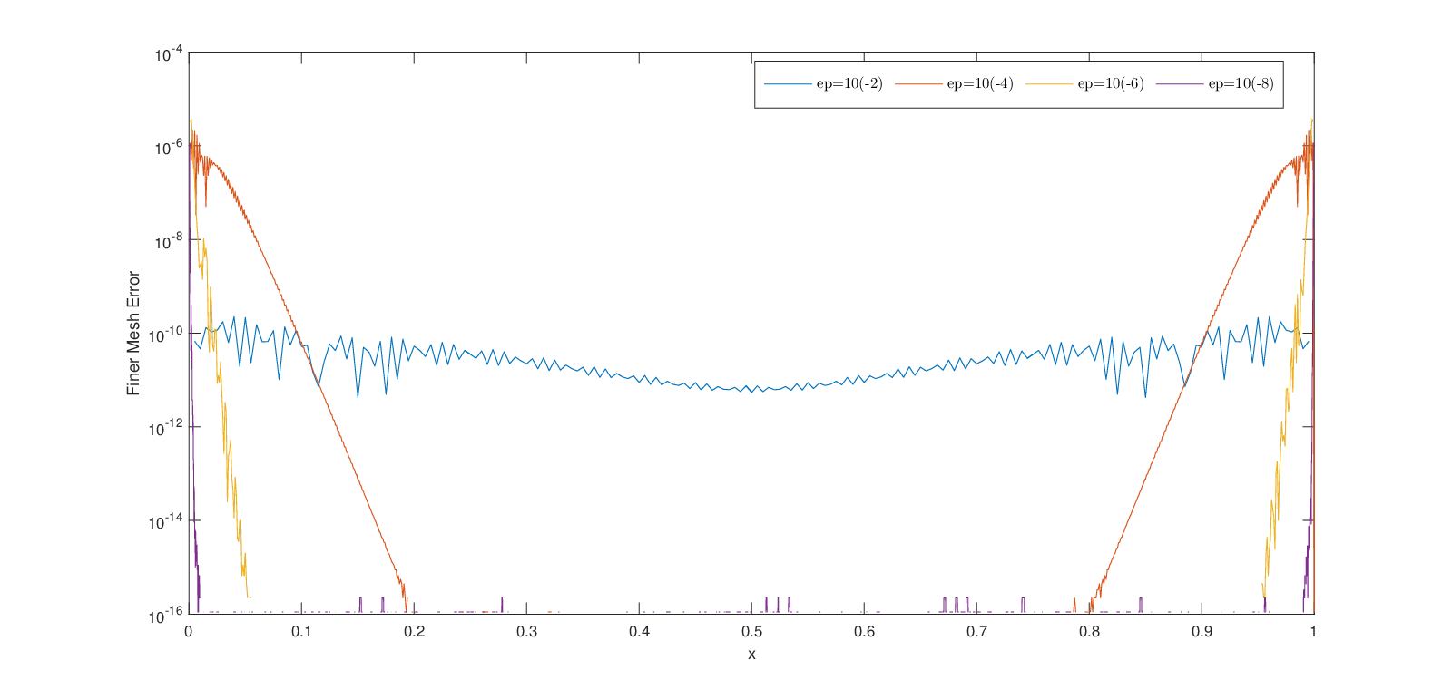
Figure 2: Errors in y1y_{1} approximations of Example 4.1 for various values of ε\varepsilon.
Example 4.2

Consider the system of coupled singularly perturbed reaction-diffusion equations [18]:

{−ε​y1′′​(x)+3​y1​(x)−y2​(x)−y3​(x)=0,−ε​y2′′​(x)−y1​(x)+3​y2​(x)−y3​(x)=1,−ε​y3′′​(x)−y2​(x)+3​y3​(x)=x,y1(0)=y1(1)=0,y2(0)=y2(1)=0,y3(0)=y3(1)=0.\left\{\begin{array}[]{ll}-\varepsilon y_{1}^{\prime\prime}\left(x\right)+3y_{1}\left(x\right)-y_{2}\left(x\right)-y_{3}\left(x\right)=0,\\[8.0pt] -\varepsilon y_{2}^{\prime\prime}\left(x\right)-y_{1}\left(x\right)+3y_{2}\left(x\right)-y_{3}\left(x\right)=1,\\[8.0pt] -\varepsilon y_{3}^{\prime\prime}\left(x\right)-y_{2}\left(x\right)+3y_{3}\left(x\right)=x,\\[8.0pt] y_{1}\left(0\right)=y_{1}\left(1\right)=0,\quad y_{2}\left(0\right)=y_{2}\left(1\right)=0,\quad y_{3}\left(0\right)=y_{3}\left(1\right)=0.\end{array}\right. (4.5)

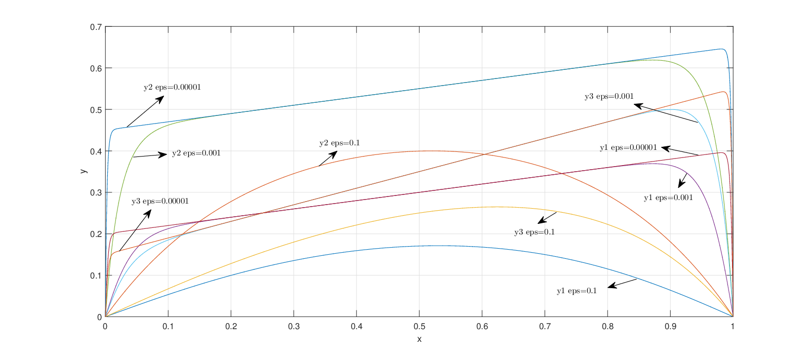
Solution of this problem exhibits boundary layer behavior in all the components y1,y_{1}, y2y_{2} and y3.y_{3}.

Refer to caption
Figure 3: SCEM approximations for Example 4.2 for certain values of ε\varepsilon.
xx y3hybridy_{3}^{\text{hybrid}} for ε=1\varepsilon=1 y3hybridy_{3}^{\text{hybrid}} for ε=0.01\varepsilon=0.01 y3hybridy_{3}^{\text{hybrid}} for ε=0.0001\varepsilon=0.0001
0.0000.000 0.0000000000000000.000000000000000 0.0000000000000000.000000000000000 0.0000000000000000.000000000000000
0.0010.001 0.0002969319142240.000296931914224 0.0015552438680930.001555243868093 0.0119078721303510.011907872130351
0.0030.003 0.0004453954373140.000445395437314 0.0046645687607070.004664568760707 0.0348078832208290.034807883220829
0.0700.070 0.0103378957224620.010337895722462 0.0989948895895990.098994889589599 0.1779465168700410.177946516870041
0.0900.090 0.0132461273871300.013246127387130 0.1217833825197110.121783382519711 0.1859949132583790.185994913258379
0.1000.100 0.0146880762813960.014688076281396 0.1322454609294060.132245460929406 0.1899984305253710.189998430525371
0.3000.300 0.0404164583595000.040416458359500 0.2639673536624640.263967353662464 0.2700000000000000.270000000000000
0.5000.500 0.0556005105022860.055600510502286 0.3482977979678310.348297797967831 0.3500000000000000.350000000000000
0.7000.700 0.0533653737359290.053365373735929 0.4174757457853870.417475745785387 0.4300000000000000.430000000000000
0.9000.900 0.0259827477797000.025982747779700 0.3606709157455800.360670915745580 0.5099968605354330.509996860535433
0.9100.910 0.0237936710585850.023793671058585 0.3442539819063670.344253981906367 0.5139898227091240.513989822709124
0.9300.930 0.0191523627508620.019152362750862 0.3023491983799680.302349198379968 0.5218928258527100.521892825852710
0.9970.997 0.0009177314280120.000917731428012 0.0202883364922930.020288336492293 0.1788127253520100.178812725352010
0.9990.999 0.0003069084784470.000306908478447 0.0068609301767900.006860930176790 0.0679329803445700.067932980344570
1.0001.000 0.0000000000000000.000000000000000 0.0000000000000000.000000000000000 0.0000000000000000.000000000000000
Table 4: Approximations to y3y_{3} of Example 4.2 for various values of ε\varepsilon, and N=1024N=1024.
ε\varepsilon N=64N=64 N=128N=128 N=256N=256 N=512N=512 N=1024N=1024
2−12^{-1} 3.97376​e−083.97376e-08 2.40516​e−092.40516e-09 1.48046​e−101.48046e-10 9.04537​e−129.04537e-12 5.14129​e−135.14129e-13
2−22^{-2} 1.60003​e−071.60003e-07 9.68587​e−099.68587e-09 5.95688​e−105.95688e-10 3.69476​e−113.69476e-11 2.45948​e−122.45948e-12
2−32^{-3} 4.55184​e−074.55184e-07 2.75605​e−082.75605e-08 1.69540​e−091.69540e-09 1.05172​e−101.05172e-10 6.50464​e−126.50464e-12
2−42^{-4} 1.86005​e−061.86005e-06 1.12657​e−071.12657e-07 6.93077​e−096.93077e-09 4.29730​e−104.29730e-10 2.67455​e−112.67455e-11
2−52^{-5} 5.30766​e−065.30766e-06 3.21668​e−073.21668e-07 1.97922​e−081.97922e-08 1.22731​e−091.22731e-09 7.63886​e−117.63886e-11
2−62^{-6} 7.19988​e−057.19988e-05 1.28455​e−061.28455e-06 7.90643​e−087.90643e-08 4.90311​e−094.90311e-09 3.05273​e−103.05273e-10
2−72^{-7} 8.50572​e−058.50572e-05 3.62682​e−063.62682e-06 2.23376​e−072.23376e-07 1.38547​e−081.38547e-08 8.62547​e−108.62547e-10
2−82^{-8} 1.48198​e−041.48198e-04 4.15936​e−054.15936e-05 8.93032​e−078.93032e-07 5.54076​e−085.54076e-08 3.44981​e−093.44981e-09
2−92^{-9} 1.20331​e−041.20331e-04 4.88494​e−054.88494e-05 2.52367​e−062.52367e-06 1.56680​e−071.56680e-07 9.75681​e−099.75681e-09
2−102^{-10} 1.12466​e−051.12466e-05 1.02047​e−041.02047e-04 2.89999​e−052.89999e-05 6.26449​e−076.26449e-07 3.90227​e−083.90227e-08
2−112^{-11} 1.42610​e−051.42610e-05 8.24795​e−058.24795e-05 3.41249​e−053.41249e-05 1.77034​e−061.77034e-06 1.10348​e−071.10348e-07
2−122^{-12} 1.25522​e−041.25522e-04 3.92817​e−063.92817e-06 7.24787​e−057.24787e-05 1.73510​e−051.73510e-05 4.41207​e−074.41207e-07
2−132^{-13} 7.95760​e−057.95760e-05 4.97760​e−064.97760e-06 7.11641​e−057.11641e-05 3.54793​e−053.54793e-05 1.24685​e−061.24685e-06
2−142^{-14} 5.17968​e−055.17968e-05 8.69193​e−058.69193e-05 1.41263​e−061.41263e-06 5.00248​e−055.00248e-05 1.43538​e−051.43538e-05
2−152^{-15} 5.35070​e−065.35070e-06 5.53248​e−055.53248e-05 1.76076​e−061.76076e-06 5.00871​e−055.00871e-05 2.50118​e−052.50118e-05
D3ND_{3}^{N} 1.48198​e−041.48198e-04 1.02047​e−041.02047e-04 7.24787​e−057.24787e-05 5.00871​e−055.00871e-05 2.50118​e−052.50118e-05
p3Np_{3}^{N} 0.53828811570.5382881157 0.49360478620.4936047862 0.53311799570.5331179957 1.00183019691.0018301969 4.79909103504.7990910350
Table 5: D3ND_{3}^{N} and p3Np_{3}^{N} for Example 4.2, for various values of ε\varepsilon and NN.
Refer to caption
Figure 4: Errors in y3y_{3} approximations of Example 4.2 for various values of ε\varepsilon.

5 Conclusion

In this paper, singularly perturbed system of two-point reaction-diffusion type boundary-value problems are examined. In order to obtain good approximations to the solution of these types of problems, a hybrid method which consists of an asymptotic method, known as SCEM and a numerical method based on finite differences given in [7] is proposed. In Section 4, the implementation of the present method is given in detail on the Illustrative Example 4.1. In Table 1, Table 2 and Table 4 numerical results that obtained by the hybrid method and in Table 3 and Table 5 maximum point-wise errors and convergence based on finer mesh strategy are presented. Additionally, approximations for some ε\varepsilon values are given in Figure 1 and Figure 3 to illustrate the layer behavior. Maximum point-wise errors for some ε\varepsilon values are given in Figure 2 and Figure 4. As one can point out from the figures and tables, that the hybrid method gives high-accurate results and well-suited for singularly perturbed system of reaction-diffusion equations.

References

  • [1] Atay MT.,Cengizci S, Eryilmaz A. SCEM approach for singularly perturbed linear turning mid-point problems with an interior layer. New Trends in Mathematical Sciences 2016; 4.1: 115-124.
  • [2] Ayaz, F. Solutions of the system of differential equations by differential transform method. Applied Mathematics and Computation 2004; 147.2: 547-567.
  • [3] Bellew S, O’Riordan E. A parameter robust numerical method for a system of two singularly perturbed convection-diffusion equations. Applied Numerical Mathematics 2004; 51.2: 171-186.
  • [4] Biazar J, Babolian E, Islam R. Solution of the system of ordinary differential equations by Adomian decomposition method. Applied Mathematics and Computation 2004; 147.3: 713-719.
  • [5] Cengizci S, Atay MT, Eryılmaz, A. A uniformly valid approximation algorithm for nonlinear ordinary singular perturbation problems with boundary layer solutions. SpringerPlus 2016; 5.1: 280.
  • [6] Cengizci S, Eryılmaz A. Successive Complementary Expansion Method for Solving Troesch’s Problem as a Singular Perturbation Problem. International Journal of Engineering Mathematics 2015; Article ID 949463.
  • [7] Cousteix J, Mauss J. Asymptotic Analysis and Boundary Layers. Scientific Computation, vol. XVIII, Springer, Berlin, Heidelberg, 2007.
  • [8] Cui M, Geng F. Solving singular two-point boundary value problem in reproducing kernel space. Journal of Computational and Applied Mathematics 2007; 205.1: 6-15.
  • [9] Das, P, Natesan, S. Optimal Error Estimate using Mesh Equidistribution Technique for Singularly Perturbed System of Reaction-Diffusion Boundary-Value Problems, Applied Mathematics and Computation, 2014; 249, 265 - 277.
  • [10] Farrell PA, Hegarty AF, Miller JJH, O’Riordan E, Shishkin GI. Robust Computational Techniques for Boundary Layers, Chapman & Hall/CRC, Boca Raton, 2000.
  • [11] Gracia JL, Lisbona FJ, O’Riordan E. A coupled system of singularly perturbed parabolic reaction-diffusion equations. Advances in Computational Mathematics 2010; 32.1: 43-61.
  • [12] Hirsch, M.W., Smale, S., and Devaney, R.L. Differential Equations, Dynamical Systems, and an Introduction to Chaos, 2004.
  • [13] Kadalbajoo MK, Gupta V. A brief survey on numerical methods for solving singularly perturbed problems,Applied Mathematics and Computation 2010; 217.8: 3641-3716.
  • [14] Kadalbajoo MK, Reddy YN. Numerical treatment of singularly perturbed two point boundary value problems, Applied mathematics and computation 1987; 21.2: 93-110.
  • [15] Kevorkian JK, Cole JD. Multiple scale and singular perturbation methods. Vol. 114. Springer Science & Business Media, 2012.
  • [16] Kumar M. Methods for solving singular perturbation problems arising in science and engineering. Mathematical and Computer Modelling 2011; 54.1-2: 556-575.
  • [17] Kumar M, Mishra HK. Variational iteration method for a singular perturbation boundary value problems. Am J Numer Anal 2014; 2.4: 102-106.
  • [18] Lin R, Stynes M. A balanced finite element method for a system of singularly perturbed reaction-diffusion two-point boundary value problems. Numerical Algorithms 2015; 70.4: 691-707.
  • [19] Linß T, Madden N. A finite element analysis of a coupled system of singularly perturbed reaction-diffusion equations. Applied mathematics and computation 2004; 148.3: 869-880.
  • [20] Linß T. Analysis of an upwind finite-difference scheme for a system of coupled singularly perturbed convection-diffusion equations. Computing 2007; 79.1: 23-32.
  • [21] Matthews S, O’Riordan E, Shishkin GI. A numerical method for a system of singularly perturbed reaction-diffusion equations. Journal of Computational and Applied Mathematics 2002; 145.1: 151-166.
  • [22] Natesan, S, Deb, B.S. A Robust Computational Method for Singularly Perturbed Coupled System of Reaction-Diffusion Boundary-Value Problems, Applied Mathematics and Computation, 2007; 188 (1), 353-364.
  • [23] Mauss J, Cousteix J. Uniformly valid approximation for singular perturbation problems and matching principle. C. R. Mécanique 2002; 330.10: 697-702.
  • [24] Miller JJH, O’Riordan E, Shishkin GI. Fitted numerical methods for singular perturbation problems: error estimates in the maximum norm for linear problems in one and two dimensions. World Scientific, 2012.
  • [25] Paramasivam M, Miller JJH, Valarmathi S. Second order parameter-uniform numerical method for a partially singularly perturbed linear system of reaction-diffusion type. Mathematical Communications 2013; 18.1: 271-295.
  • [26] Robert Jr E. Singular perturbation methods for ordinary differential equations. Vol. 89. Springer Science & Business Media, 2012.
  • [27] Shampine LF, Kierzenka J, Reichelt MW. Solving boundary value problems for ordinary differential equations in MATLAB with bvp4c. Tutorial notes, pp 437-448. http://www.mathworks.com/bvp_tutorial, 2000.
  • [28] Tamilselvan A, Ramanujam N, Shanthi V. A numerical method for singularly perturbed weakly coupled system of two second order ordinary differential equations with discontinuous source term. Journal of computational and Applied Mathematics 2007; 202.2: 203-216.
  • [29] Valanarasu T, Ramanujam N. An asymptotic initial value method for boundary value problems for a system of singularly perturbed second order ordinary differential equations. Applied Mathematics and Computation 2004; 147.1: 227-240.
  • [30] Verhulst F. Methods and applications of singular perturbations: boundary layers and multiple timescale dynamics. Vol. 50. Springer Science & Business Media, 2005.
  • [31] Vigo-Aguiar J, Natesan S. An efficient numerical method for singular perturbation problems. Journal of Computational and Applied Mathematics 2006; 192.1: 132-141.