Analysis of Lur’e dominant systems in the frequency domain
Abstract
Frequency domain analysis of linear time-invariant (LTI) systems in feedback with static nonlinearities is a classical and fruitful topic of nonlinear systems theory. We generalize this approach beyond equilibrium stability analysis with the aim of characterizing feedback systems whose asymptotic behavior is low dimensional. We illustrate the theory with a generalization of the circle criterion for the analysis of multistable and oscillatory Lur’e feedback systems.
keywords
Lur’e systems, dissipativity, circle criterion, multistability, limit cyclesfootnoteinfo]The research leading to these results has received funding from the European Research Council under the Advanced ERC Grant Agreement Switchlet n.670645. , ,
1 Introduction
Feedback systems that admit the representation in Figure 1 became seminal since the formulation of the absolute stability problem by Lur’e and Postnikov [18]. They have stimulated a great deal of research in nonlinear stability theory. Milestones include (i) the formulation of graphical conditions in the complex plane to determine necessary and sufficient conditions for absolute stability (e.g. the Nyquist criterion and the circle criterion), see e.g. [28, 29]; (ii) the equivalence between those frequency-domain conditions and linear matrix inequalities (the KYP lemma) [4]; and (iii) the characterization of input-output properties of nonlinear systems through dissipation inequalities (dissipativity theory [26] and Integral Quadratic Constraints [21]). Collectively, those developments have provided a rich analytical and computational framework to assist the search of a quadratic Lyapunov function in the global stability analysis of the feedback system.

The present paper seeks to mimic this analysis in Lur’e feedback systems that possess more general attractors than a single equilibrium. In particular, we are motivated by the analysis of multistable systems (systems with several stable equilibria) and oscillatory systems (systems with a stable limit cycle). Our analysis is differential: we look for a quadratic storage function that decreases along the solutions of the linearized system along arbitrary trajectories, possibly rescaled in time. When such a storage is positive definite, it is a differential Lyapunov function and serves to prove global contraction to a unique equilibrium [11]. Here we relax the positivity condition of the storage. Instead, we impose that the quadratic form has a given inertia : negative eigenvalues and positive eigenvalues. We use this storage to prove absolute -dominance of the Lur’e system, that is, contraction to a -dimensional attractor for all nonlinearities satisfying a differential sector condition. When , the analysis is relevant to study multistability (the one dimensional attractor being a heteroclinic orbit). When , the analysis is relevant to study limit cycles. For , the analysis boils down to the differential analysis of the absolute stability problem, pioneered by Kalman [16] and studied by many authors since then [15, 17, 22]. The main message of our paper is that the many classical tools developed in absolute stability theory to construct quadratic Lyapunov functions carry over the construction of quadratic storage with a given inertia. This means that the analysis of absolute p-dominance closely resemble the analysis of absolute stability, simply replacing the requirement of positive definiteness of the storage by a requirement on the inertia. The paper is organized as follows: the next section recalls the results of [10] dealing with -dominance in the time domain. Afterwards, the analysis of -dominance in the frequency domain is studied in Section 3, with the extensions of the Nyquist criterion and the Kalman-Yakubovich-Popov lemma for the study of -passivity as main results. These results are applied to the study of Lur’e feedback systems in the differential framework in Section 4, together with the generalization of the circle criterion. Section 5 illustrates the application of the differential framework to the study of low dimensional attractors through some examples. Finally, we end the paper with a brief section presenting conclusions and future research. Notation. Let be a real matrix, we denote the spectrum of by which is a subset of the set of complex numbers denoted by . The sets , denote the half spaces in the complex plane with positive and negative real parts respectively. The inertia of a matrix is a set of three elements containing the number of eigenvalues with positive, zero and negative real parts, respectively, that is, a matrix with inertia has eigenvalues in , eigenvalues on the -axis and eigenvalues in . Let be a complex number, then denotes the complex conjugate of . In the same way, if , then stands for the complex conjugate transpose operator, that is, , where the complex conjugate of a vector is taken element-wise.
2 Dominance in the time domain
2.1 Dominance of linear systems
A linear system
| (1) |
is -dominant if its behavior is characterized by dominant modes and transient modes, that is, if its asymptotic behavior is -dimensional. This property is of special interest if is much smaller than . One characterization of the property is via a matrix inequality with inertia constraints.
Definition 2.1
The linear system (1) is -dominant with rate if and only if there exist a symmetric matrix with inertia and such that
| (2) |
for all . The property is strict if .
The dissipation inequality (2) is equivalent to the linear matrix inequality
| (3) |
which corresponds to a standard Lyapunov inequality for the shifted matrix , with of a given inertia. Following [10, Theorem 1], for the constraint on the inertia of guarantees that the matrix has eigenvalues with strictly positive real part and eigenvalues with strictly negative real part. Indeed, the original linear system has transient modes whose convergence to zero is bounded by the rate . The remaining modes may converge to zero at exponential rate or even diverge. Those modes dominate the system behavior. Dissipativity theory [26] provides an extension of the conic constraint (2) to open systems with the state-space representation
| (4) |
where and .
Definition 2.2
The linear system (4) is -dissipative with rate and supply
| (5) |
if there exists a symmetric matrix with inertia and such that
| (6) |
for all and all . The property is strict if .
(6) is a standard dissipation inequality for the shifted system , . The classical interpretation [27] is that the supply rate bounds the variation of the storage along the trajectories of the shifted system. If the storage is positive definite, dissipativity implies stability if the supply is nonpositive. This internal property is replaced by -dominance in the case of -dissipativity. For instance, following [10] and [9], we observe that (6) is equivalent to the feasibility of the linear matrix inequality
| (7) |
A necessary condition is that the top-left element in (7) is non positive which, for , guarantees -dominance of (1). The supply rate (5) embraces many cases studied in the classical literature of dissipative systems. For example, the case and identifies the class of -passive systems. Likewise, and with correspond to strictly output -passive and strictly input -passive systems, respectively.
2.2 Dominance of nonlinear systems
Dominance is defined for nonlinear systems by making the analysis differential [8, 10, 17], i.e. by requiring dominance of the linearized system equations along arbitrary trajectories. For the nonlinear system
| (8) |
the prolonged system [5]
| (9) |
defines the linearization of the system along any of its trajectories. The intuition is that the variational trajectories capture the nonlinear behavior in an infinitesimal neighborhood of any trajectory , [8, 7].
Definition 2.3
Indeed, (10) is equivalent to finding a uniform solution to the linear matrix inequality
| (11) |
for each . Dominance strongly restricts the asymptotic behavior of the nonlinear system. -dominant systems are contractive [17, 22, 7], thus all bounded trajectories converge to a unique fixed point. -dominant systems are monotone systems [14, 1], their attractors must preserve a suitable order relation, which enforces generic convergence to fixed points. -dominant systems make contact with the property of monotonicity with respect to rank-2 cones, exploited in [25, 24] to characterize periodic attractors. The reader is referred to [9] for a thorough comparison with the literature and for a detailed analysis of the behavior of a -dominant systems. The following results from [9] justifies the interest of this paper for -dominance.
Theorem 2.4
Let (8) be a strictly -dominant system with rate . Then, the flow on any compact -limit set is topologically equivalent to a flow on a compact invariant set of a Lipschitz system in .
The theorem captures the property that the asymptotic behavior of a -dominant system is -dimensional. For , -dominance strongly constrains the possible attractors.
Corollary 2.5
In what follows we will study -dominant systems arising from the interconnection of -dissipative linear systems with static nonlinearities satisfying a differential sector condition. Theorem 2.4 and Corollary 2.5 will be particularly useful to predict the asymptotic behavior of those closed-loop systems.
3 Dominance in the frequency domain
3.1 Nyquist criterion for -dominance
Under the standing assumption of minimal realization, the poles of the transfer function of a strict -dominant system with non-negative rate are separated in two groups. The dominant poles belong to the interior of the Nyquist region
| (12) |
while the remaining poles belong to its complement. This follows directly from the separation of eigenvalues of the matrix into unstable and stable groups, which guarantees that the shifted transfer function has -poles in and poles in . The Nyquist criterion is a cornerstone of control theory for the study of closed loop stability. The principle of the argument relates the Nyquist locus of the open loop system to the position of the poles in closed loop, providing graphical conditions for closed loop stability. A similar approach can be pursued for -dominance. A straightforward application of the principle of the argument adapted to the Nyquist region provides conditions for closed loop -dominance based on the Nyquist locus of the open loop transfer function.
Theorem 3.1 (Nyquist dominance criterion)
Let be the (SISO) transfer function of a strict -dominant system with rate . Then, the closed-loop system is strictly -dominant with rate if and only if the Nyquist plot of computed along the boundary of , encircles the point , -times in the clockwise direction.
Proof of Theorem 3.1. The proof follows from Cauchy’s principle of the argument [19, Section 6.2], by taking and counting the encirclements of the origin as moves along the boundary of . Equivalently, we observe that the Nyquist plot of along the Nyquist path is the same as the Nyquist plot of along the Nyquist path , . Thus, the encirclements can be counted as varies along the -axis.
Define the closed loop transfer function given by a negative feedback loop around with gain . Take
and consider as the ratio of two polynomials . Then, and
Indeed the poles of correspond to the poles of . The zeros of correspond to the shifted closed-loop poles, given by . Hence, the number of clockwise encirclements is the difference between the number of zeros and poles of in , that is, . The result follows.
Theorem 3.1 shows that dominance of the closed loop can be determined from the Nyquist locus of the shifted transfer function . The degree of closed loop dominance is given by the difference between the clockwise encirclements of the locus around minus the number of unstable poles of . The classical Nyquist criterion for stability is recovered from the previous theorem by taking and . We note that the theorem still applies when has either poles or zeros on the -axis, using the standard indentation technique along the boundary of .
Example 3.2
Consider the linear system
| (13) |
The poles of are and . For , has poles in and 1 pole in . The Nyquist plot of along the boundary of is in Figure 2. For any positive , there are no encirclements of the point . Thus, the closed loop system formed by the negative feedback of (13) with any static gain is -dominant with rate .

The Nyquist criterion for dominance provides graphical conditions for dominance of the feedback system. More fundamentally, Theorem 3.1 shows that dominance, like stability, is shaped by feedback. Compensators can be introduced to shape the open loop transfer function with the goal of modulating the degree of dominance of the closed loop system. Likewise, dominance can be made robust, by defining dominance margins in the same way as stability margins.
3.2 Kalman-Yakubovich-Popov lemma
A key feature of dissipativity is the equivalence of the property in the time domain and in the frequency domain, characterized by the celebrated Kalman-Yakubovich-Popov lemma [23]. The same equivalence holds for -dissipativity.
Theorem 3.3 (KYP lemma for -dissipativity)
A linear system is -dissipative with rate and supply (5) if and only if, for all with , its shifted transfer function has poles in and satisfies
| (14) |
Proof of Theorem 14. Sufficiency: Assume that the system is -dissipative, and consider the complex input , . It follows that is a solution of the shifted system , , where . The following identity must then hold (we remove the dependence on for readability):
From this and (7) it follows that
Recalling that is arbitrary, (14) follows.
If the -dissipativity is strict, then (14) is also a strict inequality [2]. For Theorem 14 reduces to the standard KYP lemma, where the matrix is positive semidefinite. A classical result from the theory of passive systems, and , states that the transfer function of a passive system is positive real. For -passivity we still have that
The reader will notice this positive realness property on the Nyquist locus in Figure 2.
3.3 Geometric conditions for -passivity
The Kalman-Yakubovich-Popov lemma provides necessary geometric conditions for -passive systems in terms of the relative degree of the transfer functions and of the position of its zeros. For the next theorem we assume a single-input single-output system.
Theorem 3.4
Let (4) be a SISO -passive system with rate . Then the relative degree of its transfer function is less than or equal to and it satisfies
| (15) |
where,
-
= relative degree of , i.e., .
-
= total number of poles of .
-
= total number of finite zeros of .
-
= number of poles of in .
-
= number of finite zeros of in .
Proof of Theorem 3.4. We first recall that static feedback does not affect neither the relative degree, nor the position of the zeros of a linear system. Secondly, static negative output feedback of a -passive system preserves the -passivity of the closed-loop. Hence, the closed-loop transfer function
is -passive whenever is -passive for any , where , and are polynomials of degree , and respectively. Moreover, as increases, poles of become closer to its zeros, i.e., as . This last fact is commonly used in the construction of the root-locus [6, Chapter 6]. Assuming that is sufficiently large, the phase of approximates to
Because poles of move towards zeros in and is -passive, it follows that roots of must lie in the interior of . As a consequence
and
By Theorem 14, it follows that -passivity of implies for some and for all . Hence,
or equivalently
By noticing that and are all positive integers, the previous condition transforms into (15). To conclude the proof, assume by contradiction that , where , . It follows that the right-hand side of (15) becomes the empty set, and we get the desired contradiction. Therefore, . This ends the proof.
Table 1 shows necessary conditions for -passivity with rate in terms of , for several values of the dominance degree . In the case of classical passivity, that is, -passivity, we recover the well-known necessary condition of passivity: a passive system must be minimum phase () and its relative degree is at most one (). The poles and zeros in Table 1 refer to . In consequence their position in the complex plane depend on the value of .
| 0 | ||||
|---|---|---|---|---|
| 1 | ||||
| 2 | ||||
| 3 | ||||
| 4 | ||||
| 5 | ||||
| 6 | ||||
| 7 |
Example 3.5
Consider a system with real poles, as
| (16) |
and assume for simplicity that . By noticing that has relative degree and , it follows from Table 1 that is only compatible with -passivity and -passivity. For instance, simple computations yield,
| (17) |
Consider . By Theorem 14, a sufficient condition for -passivity of with rate is
| (18) |
Consider now . If
| (19) |
then is -passive. We will return to this example in the next section, to illustrate the design of a bistable system and of a system with a periodic attractor.
4 Differential analysis of Lur’e feedback systems in the frequency domain
4.1 Differential analysis of Lur’e systems
We will now apply the theory of the paper to a differential analysis of Lur’e systems. We look for conditions under which a Lur’e feedback system formed by a linear time-invariant system in feedback interconnection with a memoryless, time-independent nonlinearity
| (20) |
The prolonged system is given by (20) and
| (21) |
In the differential setting the usual sector condition on the nonlinearity is replaced by a sector condition on its linearization. Namely, the absolute -dominance problem consists in finding conditions under which the linear time-invariant system in feedback interconnection with memoryless, time-independent nonlinearity that satisfies the differential sector condition
| (22) |
is -dominant. The usual assumption is that and are matrices such that is symmetric positive definite. We observe that in the scalar case the sector condition (22) is in fact equivalent to require that for all . Indeed, in the differential setting, the sector condition is a restriction on the slope of the nonlinearity. Henceforth, we adopt the notation to denote the sector condition (22).
4.2 Kalman’s conjecture and conditions for -dominance of Lur’e systems
An obvious necessary condition for -dominance of (20) with the differential sector condition is -dominance of the linear system
| (23) |
for any matrix satisfying . A famous conjecture formulated by Kalman in 1957 is that this necessary condition is also sufficient. The following counterexample from [3] shows that Kalman’s conjecture fails in dimension .
Example 4.1
Consider a linear system of the form (20) where
| (24) |
Consider the static nonlinearity , where . belongs to the sector . Furthermore, the closed loop of the linear system with is asymptotically stable for any . Nevertheless, simulations show that for the initial condition the system’s trajectories display an oscillatory behavior, contradicting the stability claimed by the conjecture.
Kalman’s conjecture is an early example of differential analysis. Writing down the conditions of the conjecture within an LMI formulation shows that the condition of asymptotic stability of the linear systems with feedback gains is equivalent to the existence of a family of symmetric positive definite matrices such that
| (25) |
for . The difference between Kalman’s conjecture and (11) for strict -dominance is that (25) does not enforce a constant solution of the LMI. The dominance is only imposed pointwise, allowing for a different matrix for each gain . Indeed, Kalman conjecture provides a necessary condition for -dominance. Searching for a constant solution in (11) enforces a stronger condition than stability; it entails contraction. The breakthrough in the history of absolute stability theory came from the circle criterion, which connects a frequency domain property of the LTI system to a dissipativity property of the nonlinearity. The theorem below provides the analog sufficient condition for the -dominance of Lur’e systems.
Theorem 4.2
Proof of Theorem 4.2. From the strict dissipativity of the linear dynamics we have that the prolonged dynamics satisfies
For , using (26) we get
which shows that (10) holds along the trajectories of the prolonged closed-loop system (20),(21).
Condition (26) is in fact a generalized sector condition for the linearization . In fact, for , and we recover the differential sector condition (22). We also observe that for , and the linear system is -passive and (26) is equivalent to the condition . Indeed, the slope of the nonlinearity belongs to the sector , that is, its linearization is -passive (the nonlinearity is monotone). In this special case, Theorem 4.2 reduces to [10, Proposition 9], which provides a generalization of the passivity theorem to the context of -dissipativity.
4.3 The circle criterion for -dominance
Theorem 4.2 allows for a number of useful reformulations in the frequency domain.
Corollary 4.3
Proof of Corollary 4.3. First note that is the transfer function of
| (29) |
Hence, the fact that has poles in the interior of together with (28) allow us to apply Theorem 14, which guarantees that the prolonged dynamics of (29) satisfies
Note also that
Thus, the result follows from Theorem 4.2.
For , and , belongs to the sector and we recover (and extend to the differential setting) the standard formulation of the Positivity Theorem [13, Theorem 5.18] for . It should also be noted that the nonlinearity always satisfies the sector condition (26) if . Therefore, for , a necessary condition for the -dominance of the closed loop (20) is the dominance of linear system (4). Corollary 4.3 can be further extended via loop transformations, leading to the following reformulation of the circle criterion.
Corollary 4.4 (Multivariable Circle criterion)
Let be the transfer function of (4) and suppose that the nonlinearity satisfies (22) for some matrices such that is symmetric and positive definite. Then, the closed-loop system is strictly -dominant if the transfer function
| (30) |
has -poles in the interior of , poles in the complement of , and
| (31) |
satisfies (28).
Proof of Corollary 4.4. The proof follows directly from the loop transformation depicted in Figure 3 and Corollary 4.3. Indeed, the loop transformation arises by considering . Thus, (22) transforms into
| (32) |
In other words, satisfies (26) with , , and . Furthermore, notice that the feedback of and is equivalent to the one in Figure 3, where is as in (30). Hence, in (27) takes the form
and the result follows by Corollary 4.3.
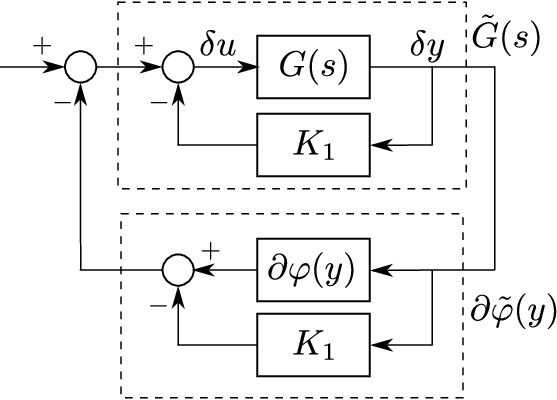
Graphical conditions can be derived for SISO systems. In the next corollary we will use to denote the Nyquist region defined in (12), and to denote the disk in the complex plane given by the set
where and are real constants.
Corollary 4.5
Consider the closed-loop system (20) given by the linear system (4) with transfer function and by a static nonlinearity . (20) is strictly -dominant if
- i)
the nonlinearity satisfies (22);
- ii)
has no poles on the boundary of ;
- iii)
the Nyquist plot of along the boundary of makes encirclements of the point in the clockwise direction, where is the number of poles of in ;
- iv)
one of the following conditions is satisfied
- (a)
and the Nyquist plot of along the boundary of lies outside of the disc .
- (b)
and the Nyquist plot of along the boundary of lies inside the disc .
- (c)
and the Nyquist plot of along the boundary of lies outside the disc .
- (a)
Proof 4.6.
The proof relies on the loop transformation of Figure 3 and Corollary 4.3. Indeed, notice that guarantees that satisfies (26) for , and . Now, define as in (27) but applied to the feedback interconnection of and , that is , where
The well-posedness of follows by . Next, by and Theorem 3.1 it follows that is strictly -dominant. Thus, it remains to prove that satisfies (28) in order to guarantee that all the assumptions of Corollary 4.3 are satisfied and the result follows. In the scalar case (28) is equivalent to
| (33) |
Let and be respectively the real and imaginary parts of , that is, . Straightforward computations reveal that (33) is equivalent to
| (34) |
for all . Now, assuming that , (34) can be rewritten as
which requires that the Nyquist plot of along the boundary of must lie outside the disc , leading to . The other two cases are similar.
The reader will recognize that the above corollaries extend the classical circle criterion to the analysis of attractors that are not necessarily fixed points. The next example shows how to use these tools to give insights on the existence of oscillatory behaviors in Lur’e systems.
Example 4.7.
We revisit Example 3.5 with , for , where , are positive real numbers. Notice that satisfies (22) with and .
Negative feedback: the closed loop is -passive. In fact, looking at the second case in Example 3.5, the transfer function of the linear part is -passive with rate satisfying (19). A direct application of the Corollary 4.5 reveals that the closed loop is -dominant whenever the Nyquist plot of along the boundary of satisfies and for any nonlinearity in the differential sector . For example, setting , and the system parameters , , , , and , it becomes clear that in Corollary 4.5 holds. Furthermore, with the selected values of parameters, it follows that has poles in , hence in Corollary 4.5 asks for encirclements of the point . Figure 4 reveals that the Nyquist plot of along the boundary of lies in , that is, and also hold for any . Hence, the -dominance of the closed-loop with rate follows. Positive feedback: in this case, the addition of the constant multiplier leads us to consider the negative feedback case as above but with . Thus, from the first part of Example 3.5 it follows that the is -passive with rate satisfying (18). From Corollary 4.5, the closed loop is -dominant whenever the Nyquist plot of along the boundary of satisfies and . For example, setting the rate and the system parameters , , , , and , it follows that the open-loop has pole in the interior of and because the Nyquist plot of falls in (see Figure 5), the conditions and hold for any , which proves -dominance of the closed-loop.


5 The asymptotic behavior of dominant Lur’e systems
In the previous sections we have extended a number of classical results to the analysis of -dominance. We will now illustrate how this analysis can be used to analyze the asymptotic behavior of Lur’e systems.
5.1 Contraction analysis (-dominance)
As a first example we briefly revisit the property of global contraction of the vector field, largely studied in the literature (see e.g., [17, 22, 12, 15] and references therein). Strict -dominance implies contraction. Indeed, Theorem 4.2 and its corollaries provide conditions for global contraction. The zero equilibrium of a Lure feedback system is then necessarily globally asymptotically stable.
5.2 Bistability (-dominance)
From Corollary 2.5, strict -dominance is a useful tool for the analysis of bistability. Global bistability of the Lure feedback system (20) is ensured from the following three properties:
- 1.
strict -dominance of the closed loop;
- 2.
boundedness of solutions; and
- 3.
the algebraic equation has three isolated solutions.
As an illustration, consider Example 4.7. Recall that, with positive feedback, any nonlinearity in the differential sector guarantees strict -dominance of the closed loop (20), with rate . This proves the -dominance. Trajectories of the closed-loop system are bounded because the input is by definition bounded and the linear system is BIBO stable. Finally, a graphical argument shows that the algebraic equation has three isolated solutions. In conclusion, we have shown that the closed-loop system formed by (16) in positive feedback interconnection with is globally bistable, that is, every solution converges to one of the three fixed points, out of which one is unstable. Figure 6 confirms the predicted behavior.

The proposed analysis is also useful for control design. If the open-loop system does not have the desired degree of dominance, a controller can be introduced to shape the frequency response in such a way that the assumptions of Corollary 4.5 are met. For illustration, we study the bistability of the Lur’e system arising from the interconnection of
| (35) |
with a saturating input-output characteristic in the differential sector . We consider the case of positive feedback. Note that the open-loop system is not -dominant for any value of rate , since it has dominant complex conjugated poles at . To achieve strict -dominance of the closed loop we enforce strict -dominance of the return ratio by pairing with a controller . Set the desired rate to and observe that has two dominant poles at and one pole at . Take . The Nyquist plot of is depicted in Figure 7. The main idea behind the selection of the controller is to increase the phase change in the Nyquist plot. By adding an unstable pole in the shifted-system, the associated Nyquist plot reflects a change in phase of 180 degrees, at zero frequency. Thus, we can set the value of the gain to achieve encirclements in the counterclockwise direction around the disk . -dominance follows. It is noteworthy that the transfer function of the desired controller reads , which is a simple first-order lag. Now, setting , the same analysis as above shows that the system has three equilibria, that all solutions are bounded and the origin is unstable. Hence, the system is bistable.

5.3 Limit cycle oscillation (-dominance)
To prove the convergence of solutions to a limit cycle in a Lure feedback system, we verify the following three conditions:
- 1.
strict -dominance of the closed loop;
- 2.
boundedness of the solutions;
- 3.
a forward invariant region that does not contain fixed points.
By Corollary 2.5, those three conditions imply that all trajectories with initial condition in the forward invariant region converge to a periodic attractor. Returning to Example 4.7, recall that the negative feedback of with any nonlinearity in the differential sector gives a strictly -dominant closed loop. We conclude that all trajectories that do not converge to the unstable fixed point necessarily converge to a limit cycle. This is illustrated Figure 8.

Remark 5.1.
The analysis of -dominance says nothing about the uniqueness of the limit cycle. As an illustration, we will verify that the system analyzed in Example 4.1 is -dominant, despite the existence of ’hidden’ oscillations. The nonlinearity satisfies the differential sector condition , with , , where . By Corollary 4.5, the closed-loop system is -dominant with rate for all the nonlinearities in the prior sector, see Figure 9.

5.4 Chaotic behavior (-dominance)
Chaotic behaviors may arise for larger dominance degree. Consider the Chua’s circuit described by
It is well known that this Lur’e system shows a chaotic behavior for certain range of parameters and nonlinearity , [20]. In fact, with the parameters , and the nonlinearity the double scroll attractor appears. An application of Corollary 4.5 shows that the interconnection is in fact -dominant with rate . Indeed, considering , the system has two complex eigenvalues in . By Corollary 4.5 it follows that the system is -dominant if the Nyquist plot encloses the disk once in the clockwise direction, as shown in Figure 10. Furthermore, the system is -passive with rate .

6 Conclusions
Dominance analysis provides sufficient conditions for the asymptotic behavior of a nonlinear system to be low-dimensional. For LTI systems, the property is verified by solving a linear matrix inequality and checking the inertia of the solution. The KYP lemma provides a frequency-domain characterization of this property. We have illustrated the potential of the frequency domain characterization in the analysis of Lure’s feedback systems. The analysis provides graphical tests for -dominance such as the circle criterion. More fundamentally, it provides robustness margins very much like in stability analysis. The theory has been illustrated on the analysis of bistable -dominant systems and oscillatory -dominant systems.
References
- [1] D. Angeli and E. Sontag. Monotone control systems. IEEE Transactions on Automatic Control, 48(10):1684 – 1698, 2003.
- [2] V. Balakrishnan and L. Vandenverghe. Semidefinite programming duality and linear time-invariant systems. IEEE Transactions on Automatic Control, 48(1):30–41, 2003.
- [3] V. O. Bragin, V. I. Vagaitsev, N. V. Kuznetsov, and G. A. Leonov. Algorithms for finding hidden oscillations in nonlinear systems. The Aizerman and Kalman conjectures and Chua’s circuits. Journal of Computer and Systems Sciences International, 50(4):511–543, 2011.
- [4] B. Brogliato, R. Lozano, B. Maschke, and O. Egeland. Dissipative Systems Analysis and Control: Theory and Applications. Communications and Control Engineering. Springer Verlag London, 2nd edition, 2007.
- [5] P. Crouch and A. van der Schaft. Variational and Hamiltonian control systems. Lecture notes in control and information sciences. Springer, 1987.
- [6] S. Engelberg. A mathematical introduction to control theory. Imperial College Press, London, 2005.
- [7] F. Forni and R. Sepulchre. A differential Lyapunov framework for contraction analysis. IEEE Transactions on Automatic Control, 59(3):614–628, 2014a.
- [8] F. Forni and R. Sepulchre. Differential analysis of nonlinear systems: revisiting the pendulum example. In Decision and Control, 53rd IEEE Conference on, pages 3848–3859, Los Angeles, USA, Dec 2014b.
- [9] F. Forni and R. Sepulchre. Differential dissipativity theory for dominance analysis. 2017a.
- [10] F. Forni and R. Sepulchre. A dissipativity theorem for -dominant systems. Submitted to the 56th IEEE Conference on Decision and Control (CDC), 2017b.
- [11] F. Forni, R. Sepulchre, and A. J. van der Schaft. On differential passivity of physical systems. In Decision and Control, 52rd IEEE Conference on, pages 6580–6585, Florence, Italy, Dec 2013.
- [12] V. Fromion and G. Scorletti. Connecting nonlinear incremental Lyapunov stability with the linearizations Lyapunov stability. In 44th IEEE Conference on Decision and Control, pages 4736 – 4741, December 2005.
- [13] W. M. Haddad and V. Chellaboina. Nonlinear dynamical systems and control: a Lyapunov-based approach. Princenton University Press, USA, 2008.
- [14] M. Hirsch and H. Smith. Monotone dynamical systems. In P. D. A. Canada and A. Fonda, editors, Handbook of Differential Equations: Ordinary Differential Equations, volume 2, pages 239 – 357. North-Holland, 2006.
- [15] J. Jouffroy and T. I. Fossen. A tutorial on incremental stability analysis using contraction theory. Modeling, Identification and Control, 31(3):93–106, 2010.
- [16] R. E. Kalman. On physical and mathematical mechanisms of instability in nonlinear automatic control systems. J. Appl. Mech. Trans. ASME, 79(3):553–566, 1957.
- [17] W. Lohmiller and J.-J. E. Slotine. On contraction analysis for nonlinear systems. Automatica, 34(6):683–696, 1998.
- [18] A. I. Lur’e and V. N. Postnikov. On the theory of stability of control systems. Applied Mathemtics and Mechanics, 8(3), 1944.
- [19] J. E. Marsden and M. J. Hoffman. Basic complex analysis. W. H. Freeman, New York, third edition, 1999.
- [20] T. Matsumoto, L. O. Chua, and M. Komuro. The double scroll. IEEE Transactions on Circuits and Systems, 32(8):797–818, 1985.
- [21] A. Megretski and A. Rantzer. System analysis via integral quadratic constraints. IEEE Trans. Autom. Control, 42(6):819–830, 1997.
- [22] A. Pavlov, N. Van De Wouw, and H. Nijmeijer. Convergent systems: analysis and synthesis. In Control and observer design for nonlinear finite and infinite dimensional systems, pages 131–146. Springer, 2005.
- [23] A. Rantzer. On the Kalman-Yakubovich-Popov lemma. Systems and Control Letters, 28:7–10, 1996.
- [24] L. Sanchez. Cones of rank 2 and the Poincaré–Bendixson property for a new class of monotone systems. Journal of Differential Equations, 246(5):1978 – 1990, 2009.
- [25] R. Smith. Existence of period orbits of autonomous ordinary differential equations. In Proceedings of the Royal Society of Edinburgh, volume 85A, pages 153–172, 1980.
- [26] J. C. Willems. Dissipative dynamical systems part I: General theory. Archive for rational mechanics and analysis, 45(5):321–351, 1972a.
- [27] J. C. Willems. Dissipative dynamical systems part II: Linear systems with quadratic supply rates. Archive for rational mechanics and analysis, 45(5):352–393, 1972b.
- [28] G. Zames. On the input-output stability of time-varying nonlinear feedback systems part I: Conditions derived using concepts of loop gain, conicity, and positivity. IEEE Transactions on Automatic Control, 11(2):228–238, 1966a.
- [29] G. Zames. On the input-output stability of time-varying nonlinear feedback systems–part II: Conditions involving circles in the frequency plane and sector nonlinearities. IEEE Transactions on Automatic Control, 11(3):465–476, 1966b.