Covers, soap films and BV functions

Giovanni Bellettini Address: Dipartimento di Ingegneria dell’Informazione e Scienze Matematiche, Università di Siena, 53100 Siena, Italy, and International Centre for Theoretical Physics ICTP, Mathematics Section, 34151 Trieste, Italy Email address: bellettini@diism.unisi.it , Maurizio Paolini Address: Dipartimento di Matematica e Fisica, Università Cattolica del Sacro Cuore, 25121 Brescia, Italy Email address: maurizio.paolini@unicatt.it , Franco Pasquarelli Address: Dipartimento di Matematica e Fisica, Università Cattolica del Sacro Cuore, 25121 Brescia, Italy Email address: franco.pasquarelli@unicatt.it and Giuseppe Scianna Address: Dipartimento di Ingegneria dell’Informazione e Scienze Matematiche, Università di Siena, 53100 Siena, Italy Email address: giuseppe.scianna@unisi.it

Date: August 24, 2026

Abstract.

In this paper we review the double covers method with constrained BV functions for solving the classical Plateau’s problem. Next, we carefully analyze some interesting examples of soap films compatible with covers of degree larger than two: in particular, the case of a soap film only partially wetting a space curve, a soap film spanning a cubical frame but having a large tunnel, a soap film that retracts onto its boundary, hence not modelable with the Reifenberg method, and various soap films spanning an octahedral frame.

1. Introduction

In [7] K. Brakke introduced the covering space method for solving a rather large class of one-codimensional Plateau type problems, including the classical case of an area-minimizing surface spanning a knot, a Steiner minimal graph connecting a given number of points in the plane, and an area-minimizing surface spanning a nonsmooth one-dimensional frame such as the one-skeleton of a polyhedron. The method does not impose any topological restriction on the solutions; it relies on the theory of currents and takes into account also unoriented objects. It consists essentially in the construction of a pair of covering spaces, and is based on the minimization of what the author called the soap film mass.

Recenlty, a slightly different approach has been proposed in [2]; it is based on the minimization of the total variation for functions defined on a single covering space and satisfying a suitable contraint on the fibers. Also this method does not impose any topological restriction on the solutions. Moreover, it takes advantage of the full machinery known on the space of BV functions defined on a locally Euclidean manifold: for instance, and remarkably, it allows approximating the considered class of Plateau type problems by $\Gamma$ -convergence. In the forthcoming paper [5] we shall deepen this $\Gamma$ -convergence regularization for finding minimal networks in the plane.

The interest in the covering space method is also illustrated in the recent paper [4], where is shown a triple cover of $\mathbb{R}^{3}\setminus(S\cup C)$ , $S$ a tetrahedral frame and $C$ two disk boundaries, compatible with a soap film spanning $S$ and having higher topological type, more precisely with two tunnels (see Figure 1 in the case of the regular tetrahedron).

Refer to caption — Figure 1. A slightly retouched version of [13, fig. 1.1.1], see also [14, fig. 11.3.2]. This soap film has two tunnels, one clearly visible in the picture. This figure was done by Jean Taylor, following an idea due to Bob Hardt.

The cover described in [4] has the particular feature of being not normal; in addition, it is constructed using the above mentioned disks. Similar disks were firstly introduced in [7] in other examples, and called invisible wires by the author. In the case of the tetrahedron, they play a crucial role. From one side, they are necessary to complete the construction of the triple cover; from the other side, they act as an obstacle. In addition, they allow one to distinguish tight loops around particular edges of the frame $S$ from loops turning far from the edges: this distinction turns out to be crucial for the modelization of a higher genus soap film. The results of [4] strongly suggest that, for a tetrahedron sufficiently elongated in one direction, the higher-genus surface has area strictly less then the conical configuration.

In this paper, for convenience of the reader we recall (Section 2) the double covers method and BV functions for treating the classical Plateau problem. In Section 3 we point out the main modifications of the construction in the case of covers of degree larger than two. Next, in Section 4 we continue the analysis in the spirit of [4], discussing various interesting examples. In Example 4.1 we discuss with some care a classical example due to F.J. Almgren of a soap film only partially wetting an unknotted curve, see also [7]. In Example 4.2 we describe a cover of $\mathbb{R}^{3}\setminus S$ , where $S$ is the one-skeleton of a cube, which is compatible with the soap film depicted in Figure 3. This is obviously not the most common soap film one usually finds in pictures, which has no holes and has triple curves starting in the corners [18, Figure 6]. It is worthwhile to notice that such a soap film has area larger than the area of the soap film in Figure 3. In Example 4.3 we show how to construct a triple cover compatible with the soap film of Figure 5, which is a surface that retracts on its boundary, and therefore for which we cannot apply the Reifenberg method. In Example 4.4 we discuss the case when $S$ is the one-skeleton of an octahedron.

We conclude this introduction by mentioning that calibrations, applied to the covering space method, have been considered in [7], [8] and, more recently, in [9] in connection with the BV approach in dimension two.

2. Double covers of $\Omega\setminus S$

In this section we describe the cut and paste method for constructing a double cover of the base space $M:=\Omega\setminus S$ where, for simplicity, $S$ is a smooth compact embedded two-codimensional manifold without boundary and $\Omega$ is a sufficiently large ball of $\mathbb{R}^{n}$ containing $S$ , $n\geq 2$ . Just to fix ideas, one can consider $n=3$ and $S$ a tame knot or link¹¹ 1 No invisible wires will be taken into account in this section.. Next, to model the area minimization problem with $S$ as boundary datum, we define a minimum problem on a class of BV functions defined on the cover and satisfying a suitable constraint. The projection over the base space of the jump set of a minimizer will be our definition of solution to the Plateau problem; this is a simplified version of the construction described in [2], to which we refer for all details. Before starting the discussion, it is worth to recall that, in more general cases (such as those in Section 4), the cut and paste procedure needs not be the most convenient method to work with. Indeed, the cover can be equivalently described in two other ways. In the first one it is sufficient to declare an orientation of the cut, and a family of permutations of the strata along the cut; this family must be consistent, a condition that is obtained from the local triviality of the cover. The second method is based on an abstract construction, by taking the quotient of the universal cover of $M$ with respect to a subgroup of the fundamental group of $M$ ; at the end of the section we recall this construction, while in Section 4 we shall use both these two latter methods.

In what follows we shall always assume that the cover is trivial in a neighbourhood of $\partial\Omega$ . Hence, in that neighbourhood we can speak without ambiguities of sheet one and sheet two, up to automorphisms of the cover.

2.1. Cut and paste construction of the double cover

We start by defining a cut (also called a cutting surface when $n=3$ ), which is a $(n-1)$ -dimensional compact embedded smooth oriented submanifold $\Sigma\subset\Omega$ with $\partial\Sigma=S$ . Next we glue two copies (the sheets, or strata) of $M:=\Omega\setminus S$ along $\Sigma$ by exchanging the sheets. Equivalently, we associate the permutation $(1\penalty\ 2)$ to $\Sigma$ .²² 2 Note that, being this permutation of order two, fixing an orientation of $\Sigma$ is not necessary and $\Sigma$ could even be nonorientable. For covers of degree larger than two and other type of permutations (see Sections 3 and 4) orientability of $\Sigma$ is necessary.

To figure out the construction, it is convenient to “double” $\Sigma$ , namely to slightly separate two copies of $\Sigma$ having boundary $S$ and meeting only at $S$ ; we call these two copies $\Sigma$ and $\Sigma^{\prime}$ , and we denote by $\mathbf{\Sigma}$ the pair $(\Sigma,\Sigma^{\prime})$ , that we call pair of cuts. The orientability of $\Sigma$ gives a unit normal vector field on $\Sigma\setminus S$ — hence, in particular, a direction to follow in order to “enlarge” the cut, separating its two “faces”. If we call $O\subset\Omega$ (resp. $I\subset\Omega$ ) the open region exterior (resp. interior) to $\Sigma\cup\Sigma^{\prime}$ , we can explicitely describe the gluing procedure as follows:

we let

$D:=\Omega\setminus\Sigma,\qquad D^{\prime}:=\Omega\setminus\Sigma^{\prime},$

and consider³³ 3 In order to be consistent with the permutation $(1\penalty\ 2)$ mentioned above, it is sufficient to rename $(D^{\prime},3)$ and $(D^{\prime},4)$ as $(D^{\prime},1)$ and $(D^{\prime},2)$ .

$\mathcal{X}:=(D,1)\cup(D,2)\cup(D^{\prime},3)\cup(D^{\prime},4);$

we endow $\mathcal{X}$ with the following equivalence relation: given $x,x^{\prime}\in M$ and $j\in\{1,2\}$ , $j^{\prime}\in\{3,4\}$ , $(x,j),(x^{\prime},j^{\prime})\in\mathcal{X}$ , we say that $(x,j)$ is equivalent to $(x^{\prime},j^{\prime})$ if and only if $x=x^{\prime}$ , and one of the following conditions hold:

(2.1)

\begin{cases}&x\in O,\qquad\{j,j^{\prime}\}\in\big\{\{1,3\},\{2,4\}\big\},\\ &x\in I,\qquad\penalty\ \{j,j^{\prime}\}\in\big\{\{1,4\},\{2,3\}\big\}.\end{cases}

We call $Y_{\mathbf{\Sigma}}$ the quotient space of $\mathcal{X}$ by this equivalence relation (endowed with the quotient topology) and $\widetilde{\pi}:\mathcal{X}\to Y_{\mathbf{\Sigma}}$ the projection. The double cover of $M$ is then

(2.2)

\pi_{\mathbf{\Sigma},M}\colon Y_{\mathbf{\Sigma}}\to M

where $\pi_{\mathbf{\Sigma},M}(\widetilde{\pi}(x,j)):=x$ for any $(x,j)\in\mathcal{X}$ , which is well defined, since if $(x,j)\sim(x^{\prime},j^{\prime})$ , then $\pi_{\mathbf{\Sigma},M}(\widetilde{\pi}(x,j))=\pi_{\mathbf{\Sigma},M}(\widetilde{\pi}(x^{\prime},j^{\prime}))$ . If we set $\pi\colon(x,j)\in\mathcal{X}\mapsto x\in M$ , we have the following commutative diagram:

(2.3)

The quotient $Y_{\mathbf{\Sigma}}$ admits a natural structure of differentiable manifold, with four local parametrizations given by $\Psi_{1},\Psi_{2},\Psi_{3},\Psi_{4}$ , where

(2.4)			$\displaystyle\Psi_{j}\colon D\to\widetilde{\pi}\big((D,j)\big),\qquad\Psi_{j}:=\widetilde{\pi}\circ\pi_{\|_{(D,j)}}^{\penalty\ \penalty\ -1},\quad j=1,2,$
(2.4)			$\displaystyle\Psi_{j^{\prime}}\colon D^{\prime}\to\widetilde{\pi}\big((D^{\prime},j^{\prime})\big),\qquad\Psi_{j^{\prime}}:=\widetilde{\pi}\circ\pi_{\|_{(D^{\prime},j^{\prime})}}^{\penalty\ \penalty\ -1},\quad j^{\prime}=3,4.$

It is important here that the transition maps are the identity:

\Psi_{j^{\prime}}^{-1}\circ\Psi_{j}=\mathrm{id}=\Psi_{j}^{-1}\circ\Psi_{j^{\prime}},\qquad j\in\{1,2\},j^{\prime}\in\{3,4\},

the equalities being valid where all members of the equation are defined. Notice that $\Psi_{1}(D)\cup\Psi_{2}(D)=Y_{\mathbf{\Sigma}}\setminus\pi_{\mathbf{\Sigma},M}^{\ -1}(\Sigma\setminus S)$ , and $\Psi_{3}(D^{\prime})\cup\Psi_{4}(D^{\prime})=Y_{\mathbf{\Sigma}}\setminus\pi_{\mathbf{\Sigma},M}^{\ -1}(\Sigma^{\prime}\setminus S)$ .

The local parametrizations allow to read a function $u:Y_{\mathbf{\Sigma}}\to\mathbb{R}$ in charts: for $j=1,2$ and $j^{\prime}=3,4$ we let $v_{j}(u):D\to\mathbb{R}$ , $v_{j^{\prime}}(u):D^{\prime}\to\mathbb{R}$ be

(2.5)

v_{j}(u):=u\circ\Psi_{j},\qquad v_{j^{\prime}}(u):=u\circ\Psi_{j^{\prime}}.

Recalling (2.1), we have

(2.6)

\begin{split}v_{1}(u)=v_{3}(u),\quad&v_{2}(u)=v_{4}(u)\qquad{\rm a.e.\penalty\ in\penalty\ }O,\\ v_{1}(u)=v_{4}(u),\quad&v_{2}(u)=v_{3}(u)\qquad{\rm a.e.\penalty\ in\penalty\ }I.\end{split}

2.2. Total variation on the double cover

The set $Y_{\mathbf{\Sigma}}$ is endowed with the push-forward $\mu$ of the $n$ -dimensional Lebesgue measure $\mathcal{L}^{n}$ in $M$ via the local parametrizations. We set $L^{1}(Y_{\mathbf{\Sigma}}):=L^{1}_{\mu}(Y_{\mathbf{\Sigma}})$ .

We say that $u$ is in $BV(Y_{\mathbf{\Sigma}})$ if its distributional gradient $Du\colon\phi\in C^{1}_{c}(Y_{\mathbf{\Sigma}})\mapsto-\int_{Y_{\mathbf{\Sigma}}}uD\phi\,d\mu\in\mathbb{R}^{n}$ is a bounded vector – valued Radon measure on $Y_{\mathbf{\Sigma}}$ . We denote by $|Du|$ the total variation measure of $Du$ .

Let $u\in BV(Y_{\mathbf{\Sigma}})$ and $E\subseteq Y_{\mathbf{\Sigma}}$ be a Borel set; $E$ can be written as the union of the following four disjoint Borel sets:

(2.7)

E\cap\widetilde{\pi}((D,1)),\;E\cap\widetilde{\pi}((D,2)),\;E\cap\widetilde{\pi}((\Sigma\setminus S,3)),\;E\cap\widetilde{\pi}((\Sigma\setminus S,4)),

and we have

(2.8)		$\displaystyle\|Du\|(E)=$	$\displaystyle\sum_{j=1,2}\|Dv_{j}(u)\|\Big(\pi_{\mathbf{\Sigma},M}\big(E\cap\widetilde{\pi}((D,j))\big)\Big)$
(2.8)			$\displaystyle+\sum_{j^{\prime}=3,4}\|Dv_{j^{\prime}}(u)\|\Big(\pi_{\mathbf{\Sigma},M}\big(E\cap\widetilde{\pi}((\Sigma\setminus S,j^{\prime}))\big)\Big).$

Notice that $\Sigma^{\prime}$ does not appear in (2.7). Choosing $D^{\prime}$ in place of $D$ amounts in considering $\Sigma^{\prime}$ in place of $\Sigma$ and does not change the subsequent discussion.

Example 2.1.

Suppose the simplest case $n=2$ , and $S$ two distinct points $q_{1},q_{2}$ . Let $u\in BV(Y_{\mathbf{\Sigma}})$ be such that $v_{1}(u)$ is equal to $a\in\mathbb{R}$ inside a disk $B$ of radius $r>0$ contained in $I$ (or in $O$ ) and $b\in\mathbb{R}$ outside, and $v_{2}(u)$ is equal to $c\in\mathbb{R}$ in $B$ and $d\in\mathbb{R}$ outside. Then, owing to (2.6),

(2.9)

\begin{split}|Du|(Y_{\mathbf{\Sigma}})=&|Dv_{1}(u)|(B\cap D)+|Dv_{2}(u)|(B\cap D)\\ &+|Dv_{3}(u)|(\Sigma\setminus\{q_{1},q_{2}\})+|Dv_{4}(u)|(\Sigma\setminus\{q_{1},q_{2}\})\\ =&(|b-a|+|d-c|)\penalty\ 2\pi r+2\mathcal{H}^{1}(\Sigma)|d-b|.\end{split}

On the other hand, if $B$ is centered at a point of $\Sigma$ , and $B\cap\Sigma^{\prime}=\emptyset$ , then

(2.10)	$\displaystyle\|Du\|(Y_{\mathbf{\Sigma}})=$	$\displaystyle\|Dv_{1}(u)\|(B\cap D)+\|Dv_{2}(u)\|(B\cap D)$
		$\displaystyle+\|Dv_{3}(u)\|(\Sigma\setminus\{q_{1},q_{2}\})+\|Dv_{4}(u)\|(\Sigma\setminus\{q_{1},q_{2}\})$
	$\displaystyle=$	$\displaystyle\left(\|b-a\|+\|d-c\|\right)\penalty\ 2\pi r+2\|c-a\|\mathcal{H}^{1}(\Sigma\cap B)$
		$\displaystyle+2\|d-b\|\left(\mathcal{H}^{1}(\Sigma)-\mathcal{H}^{1}(\Sigma\cap B)\right).$

If in particular $a=1$ , $b=0$ , $c=0$ , $d=1$ , we have that (2.9) and (2.10) become

|Du|(Y_{\mathbf{\Sigma}})=2\left(2\pi r+\mathcal{H}^{1}(\Sigma)\right).

2.3. The constrained minimum problem on the double cover

We let

BV(Y_{\mathbf{\Sigma}};\{0,1\}):=\Big\{u\in BV(Y_{\mathbf{\Sigma}})\;:\;u(y)\in\{0,1\}{\rm\penalty\ for}\penalty\ \mu\penalty\ {\rm a.e.}\penalty\ y\in Y_{\mathbf{\Sigma}}\Big\}.

The domain of $\mathcal{F}$ is defined⁴⁴ 4 For simplicity we drop the dependence on $\mathbf{\Sigma}$ in the notation. by

D(\mathcal{F}):=\Big\{u\in BV(Y_{\mathbf{\Sigma}};\{0,1\})\;:\sum_{\pi_{\mathbf{\Sigma},M}(y)=x}u(y)=1\text{\penalty\ for a.e.\penalty\ $x$ in\penalty\ }M\Big\},

and

\mathcal{F}(u):=|Du|(Y_{\mathbf{\Sigma}}),\qquad u\in D(\mathcal{F}).

Therefore the values of $u$ on the two points of a fiber are $0$ and $1$ : this is what we call the constraint on the fibers. Hence, for any $u\in D(\mathcal{F})$ we have

(2.11)

v_{1}(u)=1-v_{2}(u)\;\text{a.e.\penalty\ in}\penalty\ D,\qquad v_{3}(u)=1-v_{4}(u)\;\text{a.e.\penalty\ in}\penalty\ D^{\prime}.

For this reason, in formulas (2.12) and (2.15) below the functions $v_{2}(u)$ and $v_{4}(u)$ are not present. Moreover, the following splitting formula holds:

(2.12)

\pi_{\mathbf{\Sigma},M}(J_{u})=\Big(J_{v_{1}(u)}\setminus(\Sigma\setminus S)\Big)\cup\Big(J_{v_{3}(u)}\cap(\Sigma\setminus S)\Big).

Indeed, as in (2.7), let us split $J_{u}$ as the union of the following four disjoint sets:

(2.13)

J_{u}\cap\widetilde{\pi}((D,1)),\;J_{u}\cap\widetilde{\pi}((D,2)),\;J_{u}\cap\widetilde{\pi}((\Sigma\setminus S,3)),\;J_{u}\cap\widetilde{\pi}((\Sigma\setminus S,4)).

By the constraint on the fibers, to each point in the first set of (2.13) there corresponds a unique point in the second set, belonging to the same fiber, and viceversa. A similar correspondence holds between the third and the fourth set. Hence

\pi_{\mathbf{\Sigma},M}(J_{u})=\pi_{\mathbf{\Sigma},M}\Big(J_{u}\cap\widetilde{\pi}((D,1))\Big)\cup\pi_{\mathbf{\Sigma},M}\Big(J_{u}\cap\widetilde{\pi}((\Sigma\setminus S,3))\Big).

By the definitions of $J_{u}$ , $J_{v_{1}(u)}$ and $J_{v_{3}(u)}$ , using also the local parametrizations $\Psi_{1}$ , $\Psi_{3}$ , it follows that $\pi_{\mathbf{\Sigma},M}\big(J_{u}\cap\widetilde{\pi}((D,1))\big)=J_{v_{1}(u)}\setminus(\Sigma\setminus S)$ , and $\pi_{\mathbf{\Sigma},M}\big(J_{u}\cap\widetilde{\pi}((\Sigma\setminus S,3))\big)=J_{v_{3}(u)}\cap(\Sigma\setminus S)$ , and (2.12) follows.

Definition 2.2 (Constrained lifting).

Let $v\in BV(D;\{0,1\})$ . Then the function

(2.14)

u:=\begin{cases}v&\text{in }\Psi_{1}(D),\\ 1-v&\text{in }\Psi_{2}(D),\end{cases}

is in $D(\mathcal{F})$ , and $v_{1}(u)=v$ . We call $u$ the constrained lifting of $v$ .

In particular, when $v$ is identically equal to $1$ (or $0$ ), we have

\pi_{\mathbf{\Sigma},M}(J_{u})=\Sigma\setminus S.

The next result clarifies which is the notion of area we intend to minimize.

Proposition 2.3.

Let $u\in D(\mathcal{F})$ . Then

(2.15)

\begin{split}|Du|(Y_{\mathbf{\Sigma}})=&2\Big(\mathcal{H}^{n-1}(J_{v_{1}(u)}\setminus\Sigma)+\mathcal{H}^{n-1}(J_{v_{3}(u)}\cap\Sigma)\Big)\\ =&2\,\mathcal{H}^{n-1}(\pi_{\mathbf{\Sigma},M}(J_{u})).\end{split}

Proof.

Recall the splitting in (2.8), with the choice $E:=Y_{\mathbf{\Sigma}}$ . By (2.11), we have

(2.16)

|Dv_{1}(u)|(D)=|Dv_{2}(u)|(D),\qquad|Dv_{3}(u)|(\Sigma)=|Dv_{4}(u)|(\Sigma).

By the properties of BV functions we have

(2.17)

|Dv_{1}(u)|(D)=\mathcal{H}^{n-1}(J_{v_{1}(u)}\setminus\Sigma),\quad|Dv_{3}(u)|(\Sigma)=\mathcal{H}^{n-1}(J_{v_{3}(u)}\cap\Sigma).

Substituting (2.17) into (2.8), and recalling (2.16), we get the first equality in (2.15). The second equality is now a consequence of (2.12). ∎

Remark 2.4.

The factor $2$ in (2.15) is obtained by multiplying the absolute value of the difference of the values of $u$ (which gives a factor $1$ ), with the number of the sheets (which gives a factor $2$ ).

A particular case of a result proven in [2] is the following.

Theorem 2.5 (Existence of minimizers).

We have

(2.18)

\inf\Big\{|Du|\big(Y_{\mathbf{\Sigma}}\big)\;:\;u\in D(\mathcal{F})\Big\}=\min\Big\{|Du|\big(Y_{\mathbf{\Sigma}}\big)\;:\;u\in D(\mathcal{F})\Big\}>0.

Positivity follows from (2.20) below, with the choice $A:=\Omega$ . We denote by $u_{\min}$ a minimizer of problem (2.18).

Lemma 2.6.

Let $A\subseteq\Omega$ be a nonempty open set such that $\pi_{\mathbf{\Sigma},M}^{\ -1}(A\setminus S)$ is connected. Then for any $u\in D(\mathcal{F})$ ,

(2.19)

\mathcal{H}^{n-1}\big(A\cap\pi_{\mathbf{\Sigma},M}(J_{u})\big)>0.

Moreover, if $A$ is bounded with Lipschitz boundary, then

(2.20)

\inf\big\{\mathcal{H}^{n-1}\big(A\cap\pi_{\mathbf{\Sigma},M}(J_{u})\big)\;:\;u\in D(\mathcal{F})\big\}>0.

Proof.

By contradiction, suppose that

(2.21)

\mathcal{H}^{n-1}\big(A\cap\pi_{\mathbf{\Sigma},M}(J_{u})\big)=0.

Applying (2.12) to (2.21), we get

(2.22)

0=\mathcal{H}^{n-1}(A\cap(J_{v_{1}(u)}\setminus\Sigma))+\mathcal{H}^{n-1}(A\cap J_{v_{3}(u)}\cap\Sigma).

Now, set $A^{S}:=A\setminus S$ . Applying (2.8) with the choice $E:=\pi_{\mathbf{\Sigma},M}^{-1}(A^{S})$ , we get

(2.23)	$\displaystyle\|Du\|(\pi_{\mathbf{\Sigma},M}^{\ -1}(A^{S}))=$	$\displaystyle 2\|Dv_{1}(u)\|\left(\pi_{\mathbf{\Sigma},M}(\pi_{\mathbf{\Sigma},M}^{\ -1}(A^{S})\cap\widetilde{\pi}((D,1)))\right)$
		$\displaystyle+2\|Dv_{3}(u)\|\left(\pi_{\mathbf{\Sigma},M}(\pi_{\mathbf{\Sigma},M}^{\ -1}(A^{S})\cap\widetilde{\pi}(\Sigma\setminus S,3)))\right)$
	$\displaystyle=$	$\displaystyle 2\,\big(\|Dv_{1}(u)\|\left(A^{S}\setminus\Sigma\right)+\|Dv_{3}(u)\|\left(A^{S}\cap\Sigma\right)\big)$
	$\displaystyle=$	$\displaystyle 2\,\big(\mathcal{H}^{n-1}(A\cap(J_{v_{1}(u)}\setminus\Sigma))+\mathcal{H}^{n-1}(A\cap J_{v_{3}(u)}\cap\Sigma)\big),$

which, coupled with (2.22), implies $|Du|(\pi_{\mathbf{\Sigma},M}^{\ -1}(A^{S}))=0$ . Then $u$ is constant on $\pi_{\mathbf{\Sigma},M}^{\ -1}(A^{S})$ , which contradicts the validity of the constraint on the fibers. This proves (2.19).

Now, let us suppose, still by contradiction, that there exists a sequence $(u_{k})_{k}\subset D(\mathcal{F})$ such that $\lim_{k\to+\infty}\mathcal{H}^{n-1}\big(A\cap\pi_{\mathbf{\Sigma},M}(J_{u_{k}})\big)=0$ . Thanks to the assumption on $A$ , $\pi_{\mathbf{\Sigma},M}^{\ -1}(A^{S})$ is a double nontrivial cover of $A^{S}$ . In particular, for each $k\in\mathbb{N}$ , the restriction $\hat{u}_{k}:={u_{k}}_{|_{\pi_{\mathbf{\Sigma},M}^{\ -1}(A^{S})}}$ is in $BV(\pi_{\mathbf{\Sigma},M}^{\ -1}(A^{S});\{0,1\})$ and satisfies the constraint on the fibers, and reasoning as above, $|D{\hat{u}_{k}}|(\pi_{\mathbf{\Sigma},M}^{\ -1}(A^{S}))=2\mathcal{H}^{n-1}(A\cap\pi_{\mathbf{\Sigma},M}(J_{u_{k}}))$ . By compactness, up to a not relabelled subsequence, there exists $\hat{u}\in BV_{\mathrm{constr}}(\pi_{\mathbf{\Sigma},M}^{\ -1}(A^{S});\{0,1\})$ such that $\hat{u}_{k}\to u$ in $L^{1}(\pi_{\mathbf{\Sigma},M}^{\ -1}(A^{S}))$ , and by lower semicontinuity,

|D\hat{u}|(\pi_{\mathbf{\Sigma},M}^{\ -1}(A^{S}))\leq\liminf_{k\to+\infty}|D{\hat{u}_{k}}|(\pi_{\mathbf{\Sigma},M}^{\ -1}(A^{S}))=2\lim_{k\to+\infty}\mathcal{H}^{n-1}\big(A\cap\pi_{\mathbf{\Sigma},M}(J_{u_{k}})\big)=0.

Hence $\hat{u}$ is constant on $\pi_{\mathbf{\Sigma},M}^{\ -1}(A^{S})$ , contradicting the constraint on the fibers. ∎

Lemma 2.6 shows, in particular, that the nontrivial topology of the cover coupled with the constraint on the fibers forces $u$ to jump in suitable open sets. As a further consequence of Lemma 2.6, the boundary datum $S$ is attained by any constrained function on the cover, in the following sense.

Corollary 2.7.

Let $u\in D(\mathcal{F})$ . Then

(2.24)

\overline{\pi_{\mathbf{\Sigma},M}(J_{u})}\setminus\pi_{\mathbf{\Sigma},M}(J_{u})\supseteq S.

Proof.

The relation $S\cap\pi_{\mathbf{\Sigma},M}(J_{u})=\emptyset$ is trivial, recall also (2.12). Now, suppose by contradiction that there exists a point $p\in S\setminus\overline{\pi_{\mathbf{\Sigma},M}(J_{u})}$ . Take an open ball $B$ centered at $p$ , with $B\subset\Omega\setminus\overline{\pi_{\mathbf{\Sigma},M}(J_{u})}$ , and apply Lemma 2.6 with the choice $A:=B$ . Then, since $A\cap\pi_{\mathbf{\Sigma},M}(J_{u})=\emptyset$ , we end up with a contradiction with (2.19). ∎

If $2\leq n\leq 7$ and $u$ is a minimizer, it is possible to show that equality holds in (2.24) [2].

The definition of solution to the Plateau problem in the sense of double covers⁵⁵ 5 An analog definition can be given for covers of degree larger than two. is as follows.

Definition 2.8 (Constrained double – cover solutions).

We call

\pi_{\mathbf{\Sigma},M}(J_{u_{\rm min}})

a constrained double – cover solution (in $\Omega$ ) to Plateau’s problem with boundary $S$ .

We say that a portion $P$ of $S$ is wetted if $\overline{\pi_{\mathbf{\Sigma},M}(J_{u_{\rm min}})}\supseteq P$ , see also Section 4.

2.4. Independence of the pair of cuts

In this section we show that constrained double – cover solutions are independent of admissible cuts. A different proof of such an independence is given in Proposition 2.13.

Let us recall the definition of unoriented linking number, see for instance [6, Section 3.17] or [11, Section 5.2].

Definition 2.9.

Let $\rho\in C^{1}(\mathbb{S}^{1};\mathbb{R}^{n}\setminus S)$ be transverse to $\Sigma$ . The unoriented linking number between $\rho$ and $S$ is defined as

(2.25)

\mathrm{link}_{2}(\rho;S):=\begin{cases}0&{\rm if}\penalty\ \#(\rho^{-1}(\Sigma)){\rm\penalty\ is\penalty\ even},\\ 1&{\rm if}\penalty\ \#(\rho^{-1}(\Sigma)){\rm\penalty\ is\penalty\ odd}.\end{cases}

The right hand side of (2.25) turns out to be independent of the cut $\Sigma$ . When $\rho$ is just continuous, the unoriented linking number is defined using a $C^{1}$ loop homotopic to $\rho$ and not intersecting $S$ [11].

Theorem 2.10.

Let $\mathbf{\Sigma}=(\Sigma,\Sigma^{\prime})$ , $\mathbf{\Gamma}=(\Gamma,\Gamma^{\prime})$ be two pairs of cuts. Let $u\in BV(Y_{\mathbf{\Sigma}};\{0,1\})$ satisfies the constraint on the fibers. Then there exists $u^{\prime}\in BV(Y_{\mathbf{\Gamma}};\{0,1\})$ satisfying the constraint on the fibers such that, up to a $\mathcal{H}^{n-1}$ – negligible set,

(2.26)

\pi_{\mathbf{\Sigma},M}(J_{u})=\pi_{\mathbf{\Gamma},M}(J_{u^{\prime}}).

Proof.

Before giving the proof, we explain in a rough way the idea. First we fix a “base point” $x_{0}$ and count the parity of the number of intersections with the various manifolds $\Sigma,\Sigma^{\prime},\Gamma,\Gamma^{\prime}$ . Next, we construct $u^{\prime}$ so that $u^{\prime}$ coincides with $u$ when calculated on $(x,j)$ for $j=1,2$ , provided that the parity of the number of intersections with $\Sigma$ coincides with the parity of the number of intersections with $\Gamma$ , while $u^{\prime}$ coincides with $1-u$ when calculated on $(x,j)$ for $j=1,2$ , provided that the parity of the number of intersections with $\Sigma$ differs with the parity of the number of intersections with $\Gamma$ . Similarly, $u^{\prime}$ coincides with $u$ when calculated on $(x,j^{\prime})$ for $j^{\prime}=3,4$ , provided that the parity of the number of intersections with $\Sigma^{\prime}$ coincides with the parity of the number of intersections with $\Gamma^{\prime}$ , while $u^{\prime}$ coincides with $1-u$ when calculated on $(x,j^{\prime})$ for $j^{\prime}=3,4$ , provided that the parity of the number of intersections with $\Sigma^{\prime}$ differs with the parity of the number of intersections with $\Gamma^{\prime}$ .

Let us now come to the proof. Without loss of generality, we can suppose that $\Sigma\neq\Gamma$ . Fix $x_{0}\in M\setminus(\Sigma\cup\Gamma)$ . Let $x\in M\setminus(\Sigma\cup\Gamma)$ , and let $\gamma_{x}\in C^{1}([0,1];M)$ be such that $\gamma_{x}(0)=x_{0}$ , $\gamma_{x}(1)=x$ , and $\gamma_{x}$ is transverse both to $\Sigma$ and to $\Gamma$ ; such a $\gamma_{x}$ will be called an admissible path from $x_{0}$ to $x$ . We set

{\mathit{h}}(\gamma_{x};\Sigma,\Gamma):=\#(\gamma_{x}^{-1}(\Sigma))+\#(\gamma_{x}^{-1}(\Gamma)).

If we consider another admissible path $\lambda_{x}$ from $x_{0}$ to $x$ , we have that $h(\gamma_{x};\Sigma,\Gamma)$ and $h(\lambda_{x};\Sigma,\Gamma)$ have the same parity. Indeed, let $\rho$ be the closed curve going from $x_{0}$ to $x$ following $\gamma_{x}$ , and then backward from $x$ to $x_{0}$ along $\lambda_{x}$ . Recalling that ${\rm link}_{2}(\rho;\Sigma)={\rm link}_{2}(\rho;\Gamma)$ , it follows that ${\mathit{h}}(\gamma_{x};\Sigma,\Gamma)+{\mathit{h}}(\lambda_{x};\Sigma,\Gamma)=\#(\rho^{-1}(\Sigma))+\#(\rho^{-1}(\Gamma))$ is even. We are then allowed to set

(2.27)

h(x;\Sigma,\Gamma):=\begin{cases}0&{\rm if}\penalty\ {\mathit{h}}(\gamma_{x};\Sigma,\Gamma)\penalty\ {\rm is\penalty\ even},\\ 1&{\rm if}\penalty\ {\mathit{h}}(\gamma_{x};\Sigma,\Gamma)\penalty\ {\rm is\penalty\ odd},\end{cases}

for any admissible $\gamma_{x}$ from $x_{0}$ to $x$ ⁶⁶ 6 Once $x_{0}$ is fixed, the function $h$ allows to define an “exterior” and an “interior” of $\Sigma\cup\Gamma$ , even when $\Sigma$ and $\Gamma$ intersect on a set of positive $\mathcal{H}^{n-1}$ – measure..

Set $\mathcal{Q}:=\{x\in M\setminus(\Sigma\cup\Gamma)\;:\;h(x;\Sigma,\Gamma)=0\}$ , which is an open set, with $\partial\mathcal{Q}\subseteq\Sigma\cup\Gamma$ ; moreover $\mathcal{Q}$ has finite perimeter in $\Omega$ by [3, Proposition 3.62]. Define

v_{1}^{\prime}:=\begin{cases}v_{1}(u)\quad&\text{in }\mathcal{Q},\\ 1-v_{1}(u)\quad&\text{in }\Omega\setminus\mathcal{Q}.\end{cases}

From [3, Theorem 3.84] it follows that $v_{1}^{\prime}\in BV(\Omega;\{0,1\})$ . It also follows⁷⁷ 7 Indeed, let $x\in J_{v_{1}^{\prime}}\setminus(\Sigma\cup\Gamma)$ and let $\gamma_{x}$ be an admissible path from $x_{0}$ to $x$ . Let $B(x)$ be an open ball centered at $x$ and disjoint from $\Sigma\cup\Gamma$ ; in particular, every $z\in B(x)$ can be reached by a path obtained attaching to $\gamma_{x}$ the segment between $x$ and $z$ ; notice that such a path $\gamma_{z}$ is admissible from $x_{0}$ to $z$ , and ${\mathit{h}}(\gamma_{z};\Sigma,\Gamma)={\mathit{h}}(\gamma_{x};\Sigma,\Gamma)$ . Therefore, either $v_{1}^{\prime}=v_{1}(u)$ in $B(x)$ or $v_{1}^{\prime}=1-v_{1}(u)$ in $B(x)$ , which implies $x\in J_{v_{1}(u)}$ . Hence $J_{v_{1}^{\prime}}\setminus(\Sigma\cup\Gamma)\subseteq J_{v_{1}(u)}\setminus(\Sigma\cup\Gamma)$ . Similarly, also the converse inclusion holds, and (2.28) follows. that

(2.28)

J_{v_{1}^{\prime}}\setminus(\Sigma\cup\Gamma)=J_{v_{1}(u)}\setminus(\Sigma\cup\Gamma).

We define $u^{\prime}\in BV_{\mathrm{constr}}(Y_{\mathbf{\Gamma}};\{0,1\})$ as the constrained lifting of $v_{1}^{\prime}$ when $D$ is replaced by $\Omega\setminus\Gamma$ .

Recalling also (2.6), set

v_{3}^{\prime}:=\begin{cases}v_{1}^{\prime}&{\rm in\penalty\ the\penalty\ exterior\penalty\ region\penalty\ }{\rm\penalty\ to\penalty\ }\Gamma\cup\Gamma^{\prime},\\ 1-v_{1}^{\prime}&{\rm in\penalty\ the\penalty\ interior\penalty\ region\penalty\ }{\rm\penalty\ to\penalty\ }\Gamma\cup\Gamma^{\prime}.\end{cases}

Notice that $v^{\prime}_{3}\in BV(\Omega;\{0,1\})$ . By construction, we have

v_{1}^{\prime}=v_{1}(u^{\prime}),\qquad v_{3}^{\prime}=v_{3}(u^{\prime}).

We claim that $u^{\prime}$ satisfies (2.26). From (2.12) we have

\pi_{\mathbf{\Gamma},M}(J_{u^{\prime}})=\big(J_{v_{1}^{\prime}}\setminus(\Gamma\setminus S)\big)\cup\big(J_{v_{3}^{\prime}}\cap(\Gamma\setminus S)\big),

and our proof is concluded provided we show that, up to a $\mathcal{H}^{n-1}$ – negligible set,

(2.29)

\big(J_{v_{1}^{\prime}}\setminus\Gamma\big)\cup\big(J_{v_{3}^{\prime}}\cap\Gamma\big)=\big(J_{v_{1}(u)}\setminus\Sigma)\cup\big(J_{v_{3}(u)}\cap\Sigma\big).

Let us split the left hand side of (2.29) as follows:

(2.30)

\begin{split}J_{v_{1}^{\prime}}\setminus\Gamma&=\Big((J_{v_{1}^{\prime}}\cap\Sigma)\setminus\Gamma\Big)\cup\Big(J_{v_{1}^{\prime}}\setminus(\Sigma\cup\Gamma)\Big),\\ J_{v_{3}^{\prime}}\cap\Gamma&=\Big(J_{v_{3}^{\prime}}\cap\Sigma\cap\Gamma\Big)\cup\Big((J_{v_{3}^{\prime}}\cap\Gamma)\setminus\Sigma\Big).\end{split}

Let us show that, up to a $\mathcal{H}^{n-1}$ – negligible set,

(2.31)

(J_{v_{1}^{\prime}}\cap\Sigma)\setminus\Gamma=(J_{v_{3}(u)}\cap\Sigma)\setminus\Gamma.

Let $x\in(J_{v_{1}^{\prime}}\cap\Sigma)\setminus\Gamma$ . Up to a $\mathcal{H}^{n-1}$ -- negligible set⁸⁸ 8 Here we use again [3, Theorem 3.84]., we can assume that the approximate tangent spaces to $J_{v_{1}^{\prime}}$ and $\Sigma$ at $x$ coincide. Let $B(x)$ be an open ball centered at $x$ , not intersecting $\Gamma$ , and such that $B(x)\setminus\Sigma$ consists of two connected components. The same argument used in the proof of (2.28) shows that on one component $v_{1}^{\prime}=v_{1}(u)$ , while on the other $v_{1}^{\prime}=1-v_{1}(u)$ . Since $x\in J_{v_{1}^{\prime}}$ , we have

x\notin J_{v_{1}(u)}.

On the other hand, by (2.6), in one component we have $v_{1}(u)=v_{3}(u)$ , while in the other component $v_{3}(u)=v_{2}(u)=1-v_{1}(u)$ (where in the last equality we used (2.11)). Thus, $x\in J_{v_{3}(u)}$ . So, up to a $\mathcal{H}^{n-1}$ – negligible set, $(J_{v_{1}^{\prime}}\cap\Sigma)\setminus\Gamma\subseteq(J_{v_{3}(u)}\cap\Sigma)\setminus\Gamma$ . Arguing similarly for the other inclusion, we get (2.31).

The same argument applies also to prove that, up to a $\mathcal{H}^{n-1}$ – negligible set,

(2.32)

J_{v_{3}^{\prime}}\cap\Sigma\cap\Gamma=J_{v_{3}(u)}\cap\Sigma\cap\Gamma,\quad

and

(2.33)

(J_{v_{3}^{\prime}}\cap\Gamma)\setminus\Sigma=(J_{v_{1}(u)}\cap\Gamma)\setminus\Sigma.

From (2.28) – (2.33), we finally get (2.29). ∎

Corollary 2.11 (Independence).

The minimal value in (2.18) is independent of the pair $\mathbf{\Sigma}$ of cuts.

Proof.

Let $\mathbf{\Sigma}$ , $\mathbf{\Gamma}$ be two pairs of cuts. Let $u_{\min}\in D(\mathcal{F})$ be a function realizing the minimal value, call it $\mathscr{A}(\mathbf{\Sigma})$ . Let $u^{\prime}\in BV(Y_{\mathbf{\Gamma}};\{0,1\})$ be the function satisfying the constraint on the fibers given by Theorem 2.10 applied with $u=u_{{\rm min}}$ . Then, by (2.15) and (2.26), we have

\mathscr{A}(\mathbf{\Gamma})\leq 2\mathcal{H}^{n-1}(\pi_{\mathbf{\Gamma},M}(J_{u^{\prime}}))=2\mathcal{H}^{n-1}(\pi_{\mathbf{\Sigma},M}(J_{{u_{\min}}}))=\mathscr{A}(\mathbf{\Sigma}).

Arguing similarly for the converse inequality, we get $\mathscr{A}(\mathbf{\Gamma})=\mathscr{A}(\mathbf{\Sigma})$ . ∎

In view of Corollary 2.11, we often skip the symbol $\mathbf{\Sigma}$ in the notation of the cover, and on the minimal value of the area. Moreover, we often set

p:=\pi_{\mathbf{\Sigma},M}.

The relations between a constrained double-cover solution and other notions of solution to the Plateau problem can be found in [2].

2.5. Abstract construction of the double cover

The construction of the abstract cover is standard [10]: fix $x_{0}\in M$ , and set $C_{x_{0}}([0,1];M):=\{\gamma\in C\big([0,1];M\big)\;:\;\gamma(0)=x_{0}\}$ . For $\gamma\in C_{x_{0}}([0,1];M)$ , let $[\gamma]$ be the class of paths in $C_{x_{0}}([0,1];M)$ which are homotopic to $\gamma$ with fixed endpoints. We recall that the universal cover of $M$ is the pair $(\widetilde{M},\mathfrak{p})$ , where $\widetilde{M}:=\big\{[\gamma]\ :\ \gamma\in C_{x_{0}}([0,1];M)\big\}$ and $\mathfrak{p}\colon[\gamma]\in\widetilde{M}\mapsto\mathfrak{p}([\gamma]):=\gamma(1)\in M$ . The topology of $\widetilde{M}$ is defined as follows: consider the family $\mathcal{U}:=\{B\subseteq M\;:\;B\text{ open ball}\}$ , which is a basis of open sets of $M$ . For $B\in\mathcal{U}$ , and for $[\gamma]\in\widetilde{M}$ such that $\gamma(1)\in B$ , define

U_{[\gamma],B}:=\big\{[\gamma\lambda]\;:\;\lambda\in C([0,1];B),\;\lambda(0)=\gamma(1)\big\}.

Then a basis for the topology of $\widetilde{M}$ is given by $\widetilde{\mathcal{U}}:=\{U_{[\gamma],B}\;:\;B\in\mathcal{U},\;[\gamma]\in\widetilde{M},\,\gamma(1)\in B\}.$

Let $\pi_{1}(M,x_{0})$ be the fundamental group of $M$ with base point $x_{0}$ , and let

H:=\{[\rho]\in\pi_{1}(M,x_{0})\;:\;\mathrm{link}_{2}(\rho;S)=0\},

which is a normal subgroup of $\pi_{1}(M,x_{0})$ of index two.

For $\gamma\in C_{x_{0}}([0,1];M)$ , set $\bar{\gamma}(t):=\gamma(1-t)$ for all $t\in[0,1]$ . Associated with $H$ , we can consider the following equivalence relation $\sim_{H}$ on $\widetilde{M}$ : for $[\gamma],[\lambda]\in\widetilde{M}$ ,

[\gamma]\sim_{H}[\lambda]\iff\gamma(1)=\lambda(1),\quad\mathrm{link}_{2}(\gamma\bar{\lambda};S)=0.

We denote by $[\gamma]_{H}$ the equivalence class of $[\gamma]\in\widetilde{M}$ induced by $\sim_{H}$ , and we set

M_{H}:=\widetilde{M}/\sim_{H}.

Letting $\widetilde{\mathfrak{p}}_{H}\colon\widetilde{M}\to M_{H}$ be the canonical projection induced by $\sim_{H}$ , we endow $M_{H}$ with the corresponding quotient topology. We set $\mathfrak{p}_{H,M}\colon[\gamma]_{H}\in M_{H}\mapsto\gamma(1)\in M$ , so that we have the following commutative diagram

(2.34)

and the pair $(M_{H},\mathfrak{p}_{H,M})$ is a cover of $M$ , see [10, Proposition 1.36].

Let $(Y,\pi_{Y})$ be a cover of $M$ , and let $y_{0}\in\pi_{Y}^{-1}(x_{0})$ . By $(\pi_{Y})_{*}\colon\pi_{1}(Y,y_{0})\to\pi_{1}(M,x_{0})$ we denote the homomorphism defined as $(\pi_{Y})_{*}([\varrho]):=[\pi_{Y}\circ\varrho]$ . By [10, Proposition 1.36], we have

(2.35)

(\mathfrak{p}_{H,M})_{*}(\pi_{1}(M_{H},[x_{0}]_{H}))=H,

where $\pi_{1}(M_{H},[x_{0}]_{H})$ is the fundamental group of $M_{H}$ with base point the equivalence class $[x_{0}]_{H}$ of the constant loop $x_{0}$ .

Proposition 2.12.

Let $\mathbf{\Sigma}$ be a pair of cuts. Then $Y_{\mathbf{\Sigma}}$ and $M_{H}$ are homeomorphic.

Proof.

By [10, p. 28], we can assume that $x_{0}\notin\Sigma\cup\Sigma^{\prime}$ . Now, let $y_{0}\in\pi_{\mathbf{\Sigma},M}^{-1}(x_{0})$ and $[\varrho]\in\pi_{1}(Y_{\mathbf{\Sigma}},y_{0})$ . Then, $[\varrho]$ changes sheet in $Y_{\mathbf{\Sigma}}$ an even (or zero) number of times; therefore, assuming without loss of generality $\varrho$ of class $C^{1}$ and transverse to $\Sigma$ , recalling also (2.25), we have

0\equiv\#\big((\pi_{\mathbf{\Sigma},M}\circ\varrho)^{-1}(\Sigma)\big)\equiv\mathrm{link}_{2}(\pi_{\mathbf{\Sigma},M}\circ\varrho;S)\ \ \;(\mathrm{mod}\penalty\ 2),

which implies $\pi_{\mathbf{\Sigma},M}\circ\varrho\in H$ . Hence, $(\pi_{\mathbf{\Sigma},M})_{*}\big(\pi_{1}(Y_{\mathbf{\Sigma}},y_{0})\big)\leq H$ , and since $H$ and $(\pi_{\mathbf{\Sigma},M})_{*}\big(\pi_{1}(Y_{\mathbf{\Sigma}},y_{0})\big)$ have the same index, they must coincide. From (2.35), we deduce

(\mathfrak{p}_{H,M})_{*}(\pi_{1}(M_{H},[x_{0}]_{H}))=(\pi_{\mathbf{\Sigma},M})_{*}\big(\pi_{1}(Y_{\mathbf{\Sigma}},y_{0})\big).

By [10, Proposition 1.37], the proof is complete. ∎

The homeomorphism between the two covers, which we denote

(2.36)

f_{\mathbf{\Sigma}}\colon M_{H}\to Y_{\mathbf{\Sigma}},

is given for instance in the proof of [10, Proposition 1.33]: for $[\gamma]_{H}\in M_{H}$ , let $\beta\in C([0,1];M_{H})$ be a path from $[x_{0}]_{H}$ to $[\gamma]_{H}$ ; we uniquely lift $\mathfrak{p}_{H,M}\circ\beta$ to a path in $Y_{\mathbf{\Sigma}}$ with base point $y_{0}$ . Then, $f_{\mathbf{\Sigma}}([\gamma]_{H})$ is defined as the endpoint of the lifted path, which turns out to be independent of $\beta$ .

Let us define the distance $d_{M_{H}}$ on $M_{H}$ as follows: for $[\gamma]_{H},$ $[{\lambda}]_{H}\in M_{H}$ ,

(2.37)

d_{M_{H}}([\gamma]_{H},[\lambda]_{H}):=\inf_{\beta}\sup\big\{\sum_{l}|\mathfrak{p}_{H,M}(\beta(t_{l}))-\mathfrak{p}_{H,M}(\beta(t_{l-1}))|\;:\;(t_{l})_{l}\in\mathrm{Part}(\beta)\big\},

where the infimum runs among all $\beta\in C([0,1];M_{H})$ connecting $[\gamma]_{H}$ and $[\lambda]_{H}$ ; for any such $\beta$ , $\mathrm{Part}(\beta)$ denotes the collection of all finite partitions $(t_{l})_{l}$ of $[0,1]$ such that, for every $l$ , there exist $[\gamma_{l}]\in\widetilde{M}$ and a ball $B_{l}\subseteq M$ with $U_{[\gamma_{l}],B_{l}}\in\widetilde{\mathcal{U}}$ such that $\beta([t_{l-1},t_{l}])\subset\widetilde{\mathfrak{p}}_{H}(U_{[\gamma_{l}],B_{l}})$ .

Symmetry, positivity, and the triangular inequality of $d_{M_{H}}$ are direct consequences of the definition. Let us show that $d_{M_{H}}([\gamma]_{H},[{\lambda}]_{H})=0$ implies $[\gamma]_{H}=[{\lambda}]_{H}$ . Clearly, we have $\gamma(1)={\lambda}(1)$ . Fix $\epsilon>0$ , and let $\beta\in C([0,1],M_{H})$ , $N\in\mathbb{N}$ , $(t_{l})_{l}\in\mathrm{Part}(\beta)$ , $l\in\{1,\dots,N\}$ , be such that $\sum_{l=1}^{N}|\mathfrak{p}_{H,M}(\beta(t_{l}))-\mathfrak{p}_{H,M}(\beta(t_{l-1}))|\leq\epsilon$ . In particular, for $\epsilon>0$ sufficiently small, the closed curve $\rho$ defined as⁹⁹ 9 Here by $[\![x,x^{\prime}]\!]$ we mean the path corresponding to the segment from $x$ to $x^{\prime}$ , for every $x,\,x^{\prime}\in M$ .

\rho:=[\![\gamma(1),\mathfrak{p}_{H,M}(\beta(t_{1}))]\!]\cdots[\![\mathfrak{p}_{H,M}(\beta(t_{N-1})),\lambda(1)]\!]

is contractible in $M$ , which implies that

(2.38)

\mathrm{link}_{2}(\rho;S)=0.

By definition of ${\rm Part}(\beta)$ , for every $l\in\{1,\dots,N\}$ there exist $\lambda_{l,1}$ , $\lambda_{l,2}\in C([0,1];B_{l})$ , with $\lambda_{l,1}(0)=\lambda_{l,2}(0)=\gamma_{l}(1)$ , and such that $\beta(t_{l-1})=[\gamma_{l}\lambda_{l,1}]_{H}$ , $\beta(t_{l})=[\gamma_{l}\lambda_{l,2}]_{H}$ ; notice that, since $[\gamma_{l-1}\lambda_{l-1,2}]_{H}=\beta(t_{l-1})=[\gamma_{l}\lambda_{l,1}]_{H}$ , we have

(2.39)

\mathrm{link}_{2}(\gamma_{l-1}\lambda_{l-1,2}\bar{\lambda}_{l,1}\bar{\gamma}_{l};S)=0.

Set $\rho_{l}:=\gamma_{l}\lambda_{l,1}[\![\lambda_{l,1}(1),\lambda_{l,2}(1)]\!]\bar{\lambda}_{l,2}\bar{\gamma}_{l},$ which is a closed curve in $M$ . In particular,

(2.40)

\mathrm{link}_{2}(\rho_{l};S)=\mathrm{link}_{2}(\lambda_{l,1}[\![\lambda_{l,1}(1),\lambda_{l,2}(1)]\!]\bar{\lambda}_{l,2};S)=0,

where last equality follows recalling that $B_{l}$ is contractible in $M$ .

Coupling (2.38), (2.39) and (2.40), we get

\begin{split}\mathrm{link}_{2}(\gamma{\bar{\lambda}};S)=&\mathrm{link}_{2}(\gamma_{0}\lambda_{0,1}\bar{\lambda}_{N,2}\bar{\lambda};S)\\ =&\sum_{l=1}^{N}\Big(\mathrm{link}_{2}(\rho_{l};S)+\mathrm{link}_{2}(\gamma_{l-1}\lambda_{l-1,2}\bar{\lambda}_{l,1}\bar{\gamma}_{l};S)\Big)+\mathrm{link}_{2}(\rho;S)=0.\end{split}

Hence $[\gamma]\sim_{H}{[\lambda]}$ , and the conclusion follows.

Now, we are in the position to establish the isometry bewteen the two covers. We endow $Y_{\mathbf{\Sigma}}$ with the distance $d_{Y_{\mathbf{\Sigma}}}$ defined as follows: for any $y$ , $y^{\prime}\in Y_{\mathbf{\Sigma}}$ , we set

(2.41)

d_{Y_{\mathbf{\Sigma}}}\big(y,y^{\prime}\big)=\inf_{\eta}\ \sup\big\{\sum_{l}|\pi_{{\bf\Sigma},M}(\eta(t_{l}))-\pi_{{\bf\Sigma},M}(\eta(t_{l-1}))|\ :\ (t_{l})_{l}\in\mathrm{Part}(\eta)\big\},

where the infimum runs among all $\eta\in C([0,1];Y_{\mathbf{\Sigma}})$ connecting $y$ and $y^{\prime}$ , and $\mathrm{Part}(\eta)$ is the family of all finite partitions $(t_{l})_{l}$ of $[0,1]$ such that, for every $l$ , $\eta([t_{l-1},t_{l}])$ is contained in a single chart of $Y_{\mathbf{\Sigma}}$ .

Proposition 2.13 (Isometry).

The map $f_{\mathbf{\Sigma}}$ in (2.36) is an isometry between $(M_{H},d_{M_{H}})$ and $(Y_{\mathbf{\Sigma}},d_{Y_{\mathbf{\Sigma}}})$ .

Proof.

Let $[\gamma]_{H}$ , $[\lambda]_{H}\in M_{H}$ . For $\epsilon>0$ , let $\beta\in C([0,1];M_{H})$ be a path from $[\gamma]_{H}$ to $[\lambda]_{H}$ , realizing the infimum in (2.37) up to a contribution of order $\epsilon$ . Now, set $\eta:=f_{\mathbf{\Sigma}}\circ\beta$ ; accordingly to (2.41), let $(t_{l})_{l}\in\mathrm{Part}(\eta)$ be such that

d_{Y_{\mathbf{\Sigma}}}(f_{\mathbf{\Sigma}}([\gamma]_{H}),f_{\mathbf{\Sigma}}([\lambda]_{H}))\leq\sum_{l}|\pi_{{\bf\Sigma},M}(\eta(t_{l}))-\pi_{{\bf\Sigma},M}(\eta(t_{l-1}))|+\epsilon.

Clearly, it is not restrictive to assume that, for every $l$ , $\pi_{\mathbf{\Sigma},M}(\eta([t_{l-1},t_{l}]))\subset B_{l}$ , for some open ball $B_{l}\subset M$ . Therefore, accordingly to (2.37), we have $(t_{l})_{l}\in\mathrm{Part}(\beta)$ ; hence, for every $l$ ,

|\pi_{\mathbf{\Sigma},M}(\eta(t_{l}))-\pi_{\mathbf{\Sigma},M}(\eta(t_{l-1}))|=|\mathfrak{p}_{H,M}(\beta(t_{l}))-\mathfrak{p}_{H,M}(\beta(t_{l-1}))|,

which implies

d_{Y_{\mathbf{\Sigma}}}(f_{\mathbf{\Sigma}}([\gamma]_{H}),f_{\mathbf{\Sigma}}([\lambda]_{H}))\leq d_{M_{H}}([\gamma]_{H},[\lambda]_{H})+2\epsilon.

By the arbitrariness of $\epsilon$ , we get $d_{Y_{\mathbf{\Sigma}}}(f_{\mathbf{\Sigma}}([\gamma]_{H}),f_{\mathbf{\Sigma}}([\lambda]_{H}))\leq d_{M_{H}}([\gamma]_{H},[\lambda]_{H})$ . Similarly, we get the converse inequality. ∎

Once we have to minimize a functional defined on some functional domain, the metric structure (and not only its topology) of the cover becomes relevant: the distance function on $Y$ is locally euclidean, and the two methods described above give isometric covers.

We conclude this section remarking that a large part of what we have described can be generalized [2]:

$\bullet$

to a cover of $\mathbb{R}^{n}\setminus S$ having more then two sheets. Allowing three or more sheets has the interesting by-product of modelling singularities in soap films such as triple junctions (in the plane), or triple curves (in space), quadruple points, etc.
$\bullet$

when $S$ is not smooth, for instance $S$ the one-skeleton of a polyhedron.

We refer to [7], [2] and [4] for a more complete description for covers of any (finite) degree.

3. Covers of degree larger than two

The use of covers $p:=\pi_{\mathbf{\Sigma},M}:Y\to M$ of degree larger than two, coupled with vector-valued BV-functions defined on $Y$ and satisfying a suitable constraint, is of interest since for instance:

$\bullet$

when $n=2$ , one can model, among others, the Steiner minimal graph problem connecting a finite number $k\geq 3$ of points in the plane [2];
$\bullet$

when $n=3$ , one can consider configurations with singularities (triple curves, quadruple points etc.), in particular when $S$ is the one-dimensional skeleton of a polyhedron;
$\bullet$

choosing carefully the cover, it is possible to model soap films with higher topological genus, as in the example of the one-skeleton of a tetrahedron¹⁰¹⁰ 10 The triple cover constructed in [4] used to realize a soap film with two tunnels is not normal. Roughly, this means that one of the three sheets is treated in a special way; this is also related to the Dirichlet condition imposed on the cover in correspondence of the boundary of $\Omega$ . discussed in [4]: the resulting soap film seems not to be modelable using the Reifenberg approach [17].

Some remarks to be pointed out are the following:

$\bullet$

in the construction of the cover, and to model interesting situations, it frequently happens to make use¹¹¹¹ 11 Invisible wires can be useful also for covers of degree two. of what the author of [7] called “invisible wires”: these may have various applications, such as making globally compatible the cover, or also acting as an obstacle (see also Section 4). They are called invisible wires because the soap film should be supposed to wet the initial wireframe $S$ , but not to wet the invisible wires, so that their actual position becomes relevant. Proving that a soap film has no convenience to wet the invisible wires for special choices of their position, seems to be an open problem, not discussed in [7]. We refer to [4] for more.
$\bullet$

Instead of describing explicitely the cut and past procedure (as in Section 2) and the parametrizing maps (which becomes more and more complicated as the degree of the cover increases) now it is often convenient to construct the cover first by orienting all portions¹²¹² 12 It is worth noticing that it may happen that now the cut surface is immersed, and not embedded. of the cut, then declaring in a consistent global way the permutations for gluing the sheets along the cut, and finally to use the local triviality of the cover, in order to check the consistency of the gluing. Already in the case of triple covers, a relevant fact is the use of permutations with fixed points.
$\bullet$

Another useful way to describe the cover is the abstract construction (already considered in Section 2.5 for double covers): one has to suitably quotient the universal cover with a subgroup of the fundamental group of the complement of $S$ ¹³¹³ 13 or, if necessary, of the union of $S$ and the invisible wires.. A clear advantage of this approach is its independence of any cut, a fact that, with the cut and past procedure, requires a proof.
$\bullet$

BV-functions defined on $Y$ could be vector valued, as in [2]. Suppose for simplicity to consider a triple cover; then one choice is to work with BV-functions $u:Y\to\{\alpha,\beta,\gamma\}$ , where $\alpha,\beta,\gamma$ are the vertices of an equilateral triangle of $\mathbb{R}^{2}$ , having its barycenter at the origin. If $x$ is any point of $M$ and $p^{-1}(x)=\{y_{1},y_{2},y_{3}\}$ is the fiber over $x$ , then we require $\{u(y_{1}),u(y_{2}),u(y_{3})\}=\{\alpha,\beta,\gamma\}$ . Clearly, the constraint now reads as $\sum_{i=1}^{3}u(y_{i})=0$ .

Another choice (made also in [4]) is, instead, the following. Again, suppose for simplicity to consider a triple cover. We can consider BV-functions $u:Y\to\{0,1\}$ , so that if $x$ is any point of $M$ and $p^{-1}(x)=\{y_{1},y_{2},y_{3}\}$ is the fiber over $x$ , then we require the constraint $\sum_{i=1}^{3}u(y_{i})=1$ . Other choices of the constraint are conceivable, but we do not want to pursue this issue in the present paper.

Once we have specified the domain of the area functional, i.e., a class of constrained BV-functions $u$ , the variational problem becomes, as in Section 2, to minimize the total variation of $u$ ¹⁴¹⁴ 14 In the case of $u(y)\in\{\alpha,\beta,\gamma\}$ , the total variation is using the Frobenius norm $|T|=\sqrt{\sum(t_{ij})^{2}}$ on matrices $T=(t_{ij})$ .. This turns out to be the $(n-1)$ -dimensional Hausdorff measure of the projection $p(J_{u})$ of the jump set $J_{u}$ of $u$ , times a positive constant $c$ , related to the codomain of $u$ and possibly to the number of sheets. For instance, for $u(y)\in\{\alpha,\beta,\gamma\}$ as above, then $c=3\ell$ , where $\ell=|\beta-\alpha|$ . For $u(y)\in\{0,1\}$ , then $c=2$ .

In the next section we construct triple covers, in some interesting cases not considered in [4], and only partially considered in [7].

4. Examples

In this section all covers are of degree three; moreover, we consider BV functions $u:Y\to\{0,1\}$ with the constraint that the sum of the values of $u$ on the three points of each fiber equals $1$ .

We start with the example of Figure 2, due to F.J. Almgren [1, Fig. 1.9].

Example 4.1 (A partially wetted curve).

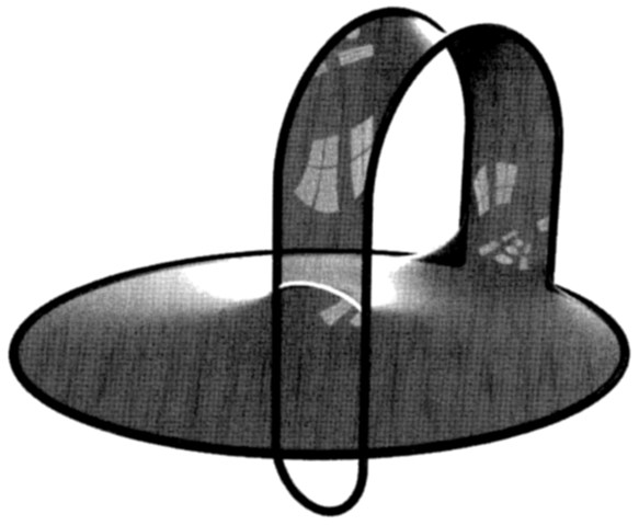
Let $S$ be the (unknotted) bold curve in Figure 2 (left). We want to construct a cover of $\mathbb{R}^{3}\setminus S$ compatible with the soap film in Figure 2 (right), where the lower part is not wetted. The presence of the triple curve suggests to use a cover of degree at least three, and indeed three will suffice. Removal of the unknotted curve from $\mathbb{R}^{3}$ leaves a set with infinite cyclic fundamental group (isomorphic to $\mathbb{Z}$ ).

The only possible cover with three sheets that can be constructed on such a base space would necessarily imply a cyclic permutation of the three points of the fiber when looping around the lower portion of the curve, forcing an undesired wetting. Similarly to the construction described in [4] and in the same spirit as in many of the examples in [7], we then add an “invisible wire” in the form of a loop circling the pair of nearby portions of $S$ in the upper part. This is represented by the dotted loop $C$ in Figure 2 (left). The base space $M$ is then defined as $\mathbb{R}^{3}\setminus(S\cup C)$ .

A cut and past construction of the cover $p:Y\to M$ can now be defined by cutting $M$ along two surfaces bounded by $S$ and by $C$ respectively. The first one resembles the film of Figure 2 (right), but it has a selfintersection along the dashed (lower) segment and continues below the disk-like portion touching the whole of $S$ ; the second one is a small disk bounded by $C$ , intersecting the first cutting surface along the dashed segment. We now take three copies, numbered $1,2,3$ , of the cutted version of $M$ and glue them along the cutting surfaces according to given permutations of the three sheets, that we now describe.

The permutation along the lower portion of $S$ is chosen as $(2\penalty\ 3)$ , namely stratum 1 glues with itself, while strata 2 and 3 get exchanged. This choice is justified because we do not want to force wetting of that portion, indeed a function in $D(\mathcal{F})$ defined equal to $1$ in sheet $1$ does not jump along a tight loop around that part of $S$ . This choice in turn requires that we fix the Dirichlet-type condition $u=1$ out of a sufficiently large ball on stratum $1$ of the cover.

The permutations on the remaining parts of the cut can then be chosen consistently as follows:

$(2\penalty\ 3)$

(as already described) in the lower tongue-like portion of the surface bordered by $S$ ;
$(2\penalty\ 3)$

when crossing the disk-like surface bordered by $C$ ;
$(1\penalty\ 2)$

when crossing the large disk-like portion of the surface bordered by $S$ ;
$(1\penalty\ 3)$

when crossing the ribbon-like portion of the surfaces between the two dashed crossing curves.

Note that corresponding to portions of the surface that are wetting the bold curve, stratum $1$ is exchanged with a different stratum.

It is a direct check that with this definition the local triviality of the triple cover around the triple curves, namely that a small loop around the dashed curves must be contractible in $M$ , is satisfied. This check consists in showing that the composition of the three permutations associated with the crossings must produce the identity: $(2\penalty\ 3)(1\penalty\ 2)^{-1}(1\penalty\ 3)^{-1}(1\penalty\ 2)=()$ . The construction is actually unique up to exchange of sheets $2$ and $3$ .

The fundamental group $\pi_{1}(M)$ of $M$ is readily seen to be free of rank $2$ . It can be generated by the two Wirtinger generators schematically denoted by $a$ and $b$ in Figure 2 left. We can then finitely present $\pi_{1}(M)$ with two generators and no relation as

\pi_{1}(M)=<a,b;>.

An abstract construction of the cover can be obtained by considering the homomorphism $\varphi:\pi_{1}(M)\to\mathcal{S}_{3}$ (permutations of the set $\{1,2,3\}$ ) defined by the position $\varphi(a)=(1\penalty\ 2)$ , $\varphi(b)=(2\penalty\ 3)$ and then defining the subgroup $H<\pi_{1}(M)$ as

H=\{w\in\pi_{1}(M):\varphi(w):1\mapsto 1\}.

It contains all reduced words $w\in\pi_{1}(M)$ whose image under $\varphi$ is either the identity $()\in\mathcal{S}_{3}$ or the transposition $(2\penalty\ 3)$ . It is a direct check that $H$ has index $3$ in $\pi_{1}(M)$ and that it is not normal.

As discussed in [4] for the example of the tetrahedral wire, also in this example we cannot exclude a priori that a minimizing surface wets the invisible wire: we have already remarked that this is a difficulty present in any example constructed using invisible wires.

Finally, we recall that soap films that partially wet any knotted curve have been proven to exist in [16].

The soap film of the next example can be found for instance in [12, pag. 85 and Fig. 4.14].

Example 4.2 (Soap film with triple curves on a cubical frame).

Let $S$ be the one-dimensional skeleton of the cube (Figure 3). We want to construct a cover of $M=\mathbb{R}^{3}\setminus S$ which is compatible with the soap film in Figure 3; note that here the soap film wets all the edges of the skeleton.

Figure 4. Left: orientation of the cut (the faces of the cube), and permutations of the sheets along the cut. Right: the Wirtinger presentation of the fundamental group of the complement of the one-skeleton of a cube.

Again, we want to model a soap film with triple curves, but not with quadruple points, and indeed, as we shall see, a triple cover of $M$ will suffice. Also, there will be no need of any invisible wire. First of all, we orient the three pairs of opposite faces of the cube from the exterior to the interior, as in Figure 4 (left). It turns out that we can make use of the cyclic permutations of $\{1,2,3\}$ . We imagine a cut along the six faces of the cube, and we associate the same permutation to opposite faces: the identity permutation $()$ is associated to the frontal and back faces, in order to model the presence of the tunnel. The three powers $(),(1\penalty\ 2\penalty\ 3),(1\penalty\ 3\penalty\ 2)$ of the cyclic permutation $(1\penalty\ 2\penalty\ 3)$ are depicted in Figure 4. The presence of the identity permutation on a pair of opposite faces has the effect of actually not having a cut there. On the other hand, a tight loop around an edge turns out in the composition of a power of $(1\penalty\ 2\penalty\ 3)$ with the inverse of a different power of $(1\penalty\ 2\penalty\ 3)$ , so that the result is either $(1\penalty\ 2\penalty\ 3)$ or $(1\penalty\ 3\penalty\ 2)$ , hence a permutation without fixed points, which forces to wet that edge.

Observe that a curve entering a face and exiting from the opposite one produces the identical permutation of the strata of the cover, hence it does not necessarily has to meet the projection of the jump set of a function $u$ .

The fundamental group of $M$ turns out to be a free group of rank $5$ , and it can be generated by the elements of $\pi_{1}(M)$ schematically displayed in Figure 4 (right) as $a$ , $b$ , $c$ , $d$ , $e$ ; the corresponding Wirtinger presentation is

\pi_{1}(M)=<a,b,c,d,e;>

(five generators and no relations). Observe that the orientation of the edges in the figure is chosen such that all five generators loop positively around the corresponding edge and result in the permutation $(1\penalty\ 2\penalty\ 3)$ of the three sheets when compared with the cut/paste construction. This allows an abstract definition of the cover by considering the homomorphism $\varphi:\pi_{1}(M)\to\mathcal{S}_{3}$ that maps all five generators onto the cyclic permutatioon $(1\penalty\ 2\penalty\ 3)$ and take the normal subgroup $H<\pi_{1}(M)$ , kernel of $\varphi$ . A word $w\in\pi_{1}(M)$ belongs to $H$ whenever the exponent sum with respect to all generators is a multiple of $3$ .

The abstract construction shows that this cover is normal. Note that this construction is invariant (up to isomorphisms) under the symmetry group of the cube, hence a minimizer will not be unique unless it is invariant under such symmetry group, which we do not expect to be true in view of the film displayed in Figure 3.

Minimizers with this topology were also obtained by real experiments [12].

The next example (Figure 5, found by J.F. Adams in [17, Appendix]) concerns a soap film which retracts to its boundary.

Example 4.3.

Let $S$ be the curve of Figure 5: we would like to consider the soap film of the figure as a cut, but in order to construct a consistent triple cover, this is not sufficient. Indeed, we add an invisible wire in the form of a loop $C$ circling around the Moëbius strip on the right; next we consider as a cut the union of the soap film in the figure and a disk bounded by $C$ . Of course, this cut has a selfintersection along a diamater of the disk. Now, take as usual three copies $1,2,3$ of the cutting surface and glue them using the permutations as follows:

$(2\penalty\ 3)$ when crossing the disk bounded by $C$ ;
$(1\penalty\ 2\penalty\ 3)$ on the remaining part of the cut.

Observe that the part of the cut on the right hand side is not orientable: the invisible wire acts in such a way to revert the cyclic permutation $(1\penalty\ 2\penalty\ 3)$ when crossing the disk.

It turns out that a presentation of the fundamental group of $M=\mathbb{R}^{3}\setminus(S\cup C)$ is

\pi_{1}(M)=<a,b;abab=baba>,

where $a$ corresponds to a small loop circling around $S$ , and $b$ corresponds to a short loop circling around the invisible wire $C$ .

The abstract definition of the cover is obtained by considering the homomorphism $\varphi:\pi_{1}(M)\to\mathcal{S}_{3}$ that maps $a$ to $(1\penalty\ 2\penalty\ 3)$ and $b$ to $(2\penalty\ 3)$ ¹⁵¹⁵ 15 One verifies that $\varphi$ is well defined with respect to the relation of the presentation.. A word belongs to $H<\pi_{1}(M)$ whenever it consists of the words of $\pi_{1}(M)$ that are mapped through $\varphi$ in a permutation of $\{1,2,3\}$ which fixes $1$ : namely, either the identity $()$ or the transposition $(2\penalty\ 3)$ .

Example 4.4.

Let $S$ be the one-skeleton of a regular octahedron. The fundamental group of $M=\mathbb{R}^{3}\setminus S$ is a free group of rank $5$ . After suitable orientation, each of the $12$ edges of the octahedron can be associated to an element of $\pi_{1}(M)$ corresponding to a loop from the base point (at infinity) that circles once in the positive sense around it.

Imposing a strong wetting condition [4] at all edges for a cover with three sheets amounts in forcing the permutation of sheets corresponding to a positive loop around that edge to be either $(1\penalty\ 2\penalty\ 3)$ or its inverse $(1\penalty\ 3\penalty\ 2)$ . Upon possibly reversing the orientation of some edge we can assume all such permutations to be $(1\penalty\ 2\penalty\ 3)$ .

Local triviality of the cover at points near a vertex then corresponds in requiring that exactly two of the four edges concurring at that vertex to be “incoming”, the other two being “outgoing”.

A choice of the orientation of the edges consistent with the requirement above corresponds to travel clockwise along the boundary edges of four of the eight faces selected in a checkerboard fashion. The resulting soap film in Figure 6 (top-left) simply consists in those four faces or on the four remaining faces.

Another consistent choice of orientation consists in travelling around the three diametral squares in a selected direction. Two relative minimizers corresponding to this choice are shown in Figure 6 (top-right and bottom), the latter consists in a tube-shaped surface with six lunettes attached along six triple curves.

It turns out that there are at least two other non isomorphic $3$ -sheeted covers of the same base space, which however seem not to provide minimizers different from the ones described above.

References

[1] F.J. Almgren, Jr. Plateau’s Problem. An Invitation to Vairfold Geometry, Revised Edition. Student Mathematical Library vol. 13, Amer. Math. Soc., 2001.
[2] S. Amato, G. Bellettini, M. Paolini: Constrained $BV$ functions on covering spaces for minimal networks and Plateau’s type problems, Adv. Calc. Var. 10 (2017), 25–47.
[3] L. Ambrosio, N. Fusco, and D. Pallara, Functions of Bounded Variation and Free Discontinuity Problems, Oxford Math. Monogr., Oxford, 2000.
[4] G. Bellettini, M. Paolini, F. Pasquarelli, Triple covers and a non-simply connected surface spanning an elongated tetrahedron and beating the cone, submitted.
[5] G. Bellettini, M. Paolini, F. Pasquarelli, G. Scianna, Singularly perturbed minimal networks using covering spaces, paper in preparation.
[6] R. Bott, and L. W. Tu, Differential Forms in Algebraic Topology, Springer – Verlag, New York, 1982.
[7] K. Brakke, Soap films and covering spaces, J. Geom. Anal. 5 (1995), 445-514.
[8] K. Brakke, Numerical solution of soap film dual problems, Exp. Math. 4 (1995), 269-287.
[9] M. Carioni, A. Pluda, Calibrations for minimal networks in a covering space setting, arXiv:1707.01448v1.
[10] A. E. Hatcher, Algebraic Topology, Cambridge University Press, Cambridge, 2001.
[11] M. W. Hirsch, Differential Topology, Springer – Verlag, New York, 1976.
[12] C. Isenberg, The Science of Soap Films and Soap Bubbles, Dover Publications, Inc., New York, 1992.
[13] G. Lawlor, F. Morgan, Paired calibrations applied to soap films, immiscible fluids, and surfaces or networks minimizing other norms, Pacific J. Math. 166 (1994), 55–83.
[14] F. Morgan, Geometric Measure Theory: A Beginners Guide, Elsevier Science, 2008.
[15] F. Morgan, Soap films and mathematics, Proc. Symp. Pure Math. 54 (1993), 375–380.
[16] H.R. Parks, Soap-film-like minimal surfaces spanning knots, J. Geom. Anal. 2 (1992), 267–290.
[17] E.R. Reifenberg, Solution of the Plateau problem for m-dimensional surfaces of varying topological type, Acta Math. 104 (1960), 1–92 (Appendix by J. Frank Adams).
[18] J. Taylor, The structure of singularities in soap-bubble-like and soap-film-like minimal surfaces, Ann. Math. 103 (1976), 489–539.

(2.8)		$\displaystyle\|Du\|(E)=$	$\displaystyle\sum_{j=1,2}\|Dv_{j}(u)\|\Big(\pi_{\mathbf{\Sigma},M}\big(E\cap\widetilde{\pi}((D,j))\big)\Big)$
(2.8)			$\displaystyle+\sum_{j^{\prime}=3,4}\|Dv_{j^{\prime}}(u)\|\Big(\pi_{\mathbf{\Sigma},M}\big(E\cap\widetilde{\pi}((\Sigma\setminus S,j^{\prime}))\big)\Big).$

(2.10)	$\displaystyle\|Du\|(Y_{\mathbf{\Sigma}})=$	$\displaystyle\|Dv_{1}(u)\|(B\cap D)+\|Dv_{2}(u)\|(B\cap D)$
		$\displaystyle+\|Dv_{3}(u)\|(\Sigma\setminus\{q_{1},q_{2}\})+\|Dv_{4}(u)\|(\Sigma\setminus\{q_{1},q_{2}\})$
	$\displaystyle=$	$\displaystyle\left(\|b-a\|+\|d-c\|\right)\penalty\ 2\pi r+2\|c-a\|\mathcal{H}^{1}(\Sigma\cap B)$
		$\displaystyle+2\|d-b\|\left(\mathcal{H}^{1}(\Sigma)-\mathcal{H}^{1}(\Sigma\cap B)\right).$

Covers, soap films and BV functions

Abstract.

1. Introduction

2. Double covers of Ω∖S\Omega\setminus S

2.1. Cut and paste construction of the double cover

2.2. Total variation on the double cover

Example 2.1.

2.3. The constrained minimum problem on the double cover

Definition 2.2 (Constrained lifting).

Proposition 2.3.

Proof.

Remark 2.4.

Theorem 2.5 (Existence of minimizers).

Lemma 2.6.

Proof.

Corollary 2.7.

Proof.

Definition 2.8 (Constrained double – cover solutions).

2.4. Independence of the pair of cuts

Definition 2.9.

Theorem 2.10.

Proof.

Corollary 2.11 (Independence).

Proof.

2.5. Abstract construction of the double cover

Proposition 2.12.

Proof.

Proposition 2.13 (Isometry).

Proof.

3. Covers of degree larger than two

4. Examples

Example 4.1 (A partially wetted curve).

Example 4.2 (Soap film with triple curves on a cubical frame).

Example 4.3.

Example 4.4.

References

2. Double covers of $\Omega\setminus S$