跳到论文正文
W Papers独立论文阅读器 arXiv:1710.01566 论文正文 计算阅读时间 · 0%
引用这篇论文根据当前论文元数据生成,正式投稿前建议核对。


License: arXiv.org perpetual non-exclusive license
arXiv:1710.01566v1 [math.AP] 04 Oct 2017

First-order, stationary mean-field games with congestionThanks:  The authors were partially supported by King Abdullah University of Science and Technology (KAUST) baseline and start-up funds.

David Evangelista D. Evangelista King Abdullah University of Science and Technology (KAUST), CEMSE Division , Thuwal 23955-6900. Saudi Arabia, and KAUST SRI, Center for Uncertainty Quantification in Computational Science and Engineering. Email address: david.evangelista@kaust.edu.sa , Rita Ferreira R. Ferreira King Abdullah University of Science and Technology (KAUST), CEMSE Division, Thuwal 23955-6900. Saudi Arabia, and KAUST SRI, Center for Uncertainty Quantification in Computational Science and Engineering. Email address: rita.ferreira@kaust.edu.sa , Diogo A. Gomes D. A. Gomes King Abdullah University of Science and Technology (KAUST), CEMSE Division, Thuwal 23955-6900. Saudi Arabia, and KAUST SRI, Center for Uncertainty Quantification in Computational Science and Engineering. Email address: diogo.gomes@kaust.edu.sa , Levon Nurbekyan L. Nurbekyan King Abdullah University of Science and Technology (KAUST), CEMSE Division, Thuwal 23955-6900. Saudi Arabia, and KAUST SRI, Center for Uncertainty Quantification in Computational Science and Engineering. Email address: levon.nurbekyan@kaust.edu.sa and Vardan Voskanyan V. Voskanyan King Abdullah University of Science and Technology (KAUST), CEMSE Division, Thuwal 23955-6900. Saudi Arabia, and KAUST SRI, Center for Uncertainty Quantification in Computational Science and Engineering. Email address: vardan.voskanyan@kaust.edu.sa
Date: August 24, 2026
Abstract.

Mean-field games (MFGs) are models for large populations of competing rational agents that seek to optimize a suitable functional. In the case of congestion, this functional takes into account the difficulty of moving in high-density areas.

Here, we study stationary MFGs with congestion with quadratic or power-like Hamiltonians. First, using explicit examples, we illustrate two main difficulties: the lack of classical solutions and the existence of areas with vanishing density. Our main contribution is a new variational formulation for MFGs with congestion. This formulation was not previously known, and, thanks to it, we prove the existence and uniqueness of solutions. Finally, we consider applications to numerical methods.

Key words and phrases: 
Mean-Field Game; Congestion; Calculus of Variations
2010 Mathematics Subject Classification
35J47, 35A01

1. Introduction

Mean-field games (MFGs) is a branch of game theory that studies systems with a large number of competing agents. These games were introduced in [28, 29, 30] (see also [31]) and [26, 27] motivated by problems arising in population dynamics, mathematical economics, social sciences, and engineering. MFGs have been the focus of intense study in the last few years and substantial progress has been achieved. Congestion problems, which arise in models where the motion of agents in high-density regions is expensive, are a challenging class of MFGs. Many MFGs are determined by a system of a Hamilton–Jacobi equation coupled with a transport or Fokker–Planck equation. In congestion problems, these equations have singularities and, thus, their analysis requires particular care.

Here, we study first-order stationary MFGs with congestion. Our main example is the system

(1.1) {|P+D​u|γγ​mα+V⁡(x)=g⁡(m)+H¯−div⁡(m1−α​|P+D​u|γ−2​(P+D​u))=0,\begin{cases}\frac{|P+Du|^{\gamma}}{\gamma m^{\alpha}}+V(x)=g(m)+{\overline{H}}\\ -\operatorname{div}(m^{1-\alpha}|P+Du|^{\gamma-2}(P+Du))=0,\end{cases}

where xx takes values on the dd-dimensional torus, 𝕋d{\mathbb{T}}^{d}, and the unknowns are u,m:𝕋d→ℝu,m:{\mathbb{T}}^{d}\to{\mathbb{R}} and H¯∈ℝ{\overline{H}}\in{\mathbb{R}}, with m⩾0m\geqslant 0 and ∫𝕋dm​𝑑x=1\int_{{\mathbb{T}}^{d}}m\,dx=1. Here, 1⩽α⩽γ<∞1\leqslant\alpha\leqslant\gamma<\infty, V:𝕋d→ℝV:{\mathbb{T}}^{d}\to{\mathbb{R}}, V∈C∞​(𝕋d)V\in C^{\infty}({\mathbb{T}}^{d}), and g:ℝ+→ℝg:{\mathbb{R}}^{+}\to{\mathbb{R}} with g​(m)=G′​(m)g(m)=G^{\prime}(m) for some convex function G:ℝ0+→ℝG:{\mathbb{R}}_{0}^{+}\to{\mathbb{R}} with G∈C∞​(ℝ+)∩C⁡(ℝ0+)G\in C^{\infty}({\mathbb{R}}^{+})\cap C({\mathbb{R}}_{0}^{+}). In particular, the convexity of GG gives that gg is monotonically increasing.

The preceding MFG is a model where agents incur in a large cost if moving in regions with a high agent density. The constant −H¯-{\overline{H}} is the average cost per unit of time corresponding to the Lagrangian

L⁡(x,v,m)=mα​|v|γ′γ′+v⋅P−V⁡(x)+g⁡(m),L(x,v,m)=m^{\alpha}\frac{|v|^{\gamma^{\prime}}}{\gamma^{\prime}}+v\cdot P-V(x)+g(m),

where 1γ+1γ′=1\frac{1}{\gamma}+\frac{1}{\gamma^{\prime}}=1. More precisely, the typical agent seeks to minimize the long-time average cost

limT→∞1T​∫0T(mα​|𝐱˙​(s)|γ′γ′+𝐱˙​(s)⋅P−V⁡(𝐱⁡(s))+g⁡(m⁡(𝐱⁡(s))))​𝑑s.\lim_{T\to\infty}\frac{1}{T}\int_{0}^{T}\bigg(m^{\alpha}\frac{|\dot{\bf x}(s)|^{\gamma^{\prime}}}{\gamma^{\prime}}+\dot{\bf x}(s)\cdot P-V({\bf x}(s))+g(m({\bf x}(s)))\bigg)ds.

Due to this optimization process, agents avoid moving in high-density regions. Further, because gg is increasing, agents prefer to remain in low-density regions rather than in high-density regions. Finally, we observe that PP determines the preferred direction of motion.

In the stationary case, the theory for second-order MFGs without singularities is well understood. For example, the papers [20, 18, 16, 34, 19] address the existence of classical solutions and weak solutions were examined in [4]. In dimension one, a characterization of solutions for stationary MFGs was developed in [15] (including non-monotone MFGs) and, in the case of congestion, in [14, 33]. The theory of weak solutions was considered in [11], where a general existence result was proven using a monotonicity argument. The monotonicity structure that many MFGs enjoy has important applications to numerical methods, see [2]. A review of MFG models can be found in [21] and a survey of regularity results in [17].

The congestion problem was first introduced in [31] where a uniqueness condition was established. Next, the existence problem for stationary MFGs with congestion, positive viscosity, and a quadratic Hamiltonian was proved in [13]. Subsequently, this problem was examined in more generality in [9]. The time-dependent case was considered in [22] (classical solutions) and [23] (weak solutions). Later, [1] examined weak solutions for time-dependent problems.

Apart from the results in [11], the one-dimensional examples in [14, 33], and the radial cases in [10], little is known about first-order MFGs with congestion. The critical difficulties stem from two issues: first-order Hamilton–Jacobi equations provide little a priori regularity; second, because the transport equation is a first-order equation, we cannot use Harnack-type results and, thus, we cannot bound mm by below by a positive constant. Indeed, as we show in Section 2.1, mm can vanish. In many MFG problems, the regularity follows from a priori bounds that combine both equations in (1.1). Here, with standard methods, we can only get relatively weak bounds, see Remark 3.6. For example, if 0<α⩽10<\alpha\leqslant 1, then there exists a constant, CC, such that for any regular enough solution of (1.1), we have

∫𝕋d[(|P+D​u|γmα)​(1+m)+(m−1)​g​(m)]​𝑑x⩽C.\int_{{\mathbb{T}}^{d}}\left[\left(\frac{|P+Du|^{\gamma}}{m^{\alpha}}\right)(1+m)+(m-1)g(m)\right]dx\leqslant C.

In Section 3, we examine a priori bounds for a class of MFGs that generalize (1.1).

While the bounds from Section 3 are interesting on their own, they are not enough to prove the existence of solutions. In the case of MFGs without congestion, a number of variational principles have been proposed, see [28, 31]. These are not only of independent interest but also have important applications, see, for example, [36] for a study of efficiency loss in oscillator synchronization games, the recent results in [5] where variational principles are used to prove the existence of solutions for first-order MFGs, and [3] where optimal transport methods are used to examine constrained MFGs, which is an alternative approach to model congestion. Hard congestion problems can be modeled by variational problems, see for example [35] or [6]. However, soft-congestion models such as (1.1) do not fit this framework. In Section 4, we study a new variational problem for which (1.1) is the corresponding Euler–Lagrange equation. More concretely, let G:ℝ0+→ℝG:{\mathbb{R}}_{0}^{+}\to{\mathbb{R}} with G′=gG^{\prime}=g. Then, (1.1) is the Euler–Lagrange equation of the functional

(1.2) J⁡[u,m]=∫𝕋d(|P+D​u|γγ⁡(α−1)​mα−1−V​m+G⁡(m))​𝑑x;J[u,m]=\int_{{\mathbb{T}}^{d}}\left(\frac{|P+Du|^{\gamma}}{\gamma(\alpha-1)m^{\alpha-1}}-Vm+G(m)\right)dx;

that is, if (u,m)(u,m), with u,m:𝕋d→ℝu,m:{\mathbb{T}}^{d}\to{\mathbb{R}} and m>0m>0, is a smooth enough minimizer of JJ under the constraint

∫𝕋dm​𝑑x=1,\int_{{\mathbb{T}}^{d}}m\,dx=1,

then (u,m)(u,m) solves (1.1). The existence of a minimizer of (1.2) is addressed as follows. First, the α=1\alpha=1 case is examined in Section 2.2. The 1<α<γ1<\alpha<\gamma case and the case where α=γ\alpha=\gamma with g=mθg=m^{\theta}, θ>0\theta>0, are addressed in Theorem 4.6. Finally, the α=γ\alpha=\gamma with more general assumptions on gg case is considered in Theorem 4.8. The uniqueness of a solution is shown in Theorem 4.9. Our new variational principle provides a new construction of weak solutions for MFGs that does not rely on the high-order regularizations in [11] nor requires ellipticity as in [16, 18, 19, 20, 34]. Moreover, our methods suggest an alternative computational approach for stationary MFGs with congestion that complements the existing ones, see [2].

Our variational methods do not apply for 0<α<10<\alpha<1 nor to second-order MFGs. Sections 5 and 6 are devoted to the study of these cases. In Section 5, we examine first-order MFGs with 0<α<10<\alpha<1 in the two-dimensional case. There, we perform a change of variables for which our variational methods can be used. Next, in Section 6, we study various cases where we can reduce second-order MFG systems to scalar equations. Moreover, we show that these equations are equivalent to Euler–Lagrange equations of suitable functionals. Finally, in Sections 7–9, we use our results to develop numerical methods for MFGs.

2. Some explicit examples

Before developing the general theory, we consider three examples that illustrate some of the properties of (1.1). First, we prove that (1.1) may fail to have classical solutions. Next, we examine the critical congestion case, α=1\alpha=1. In this case, uu is constant and the existence of solutions to (1.1) can be addressed by solving algebraic equations.

2.1. Lack of classical solutions

In general, (1.1) may not have classical solutions. To illustrate this behavior, we consider the case when P=0,P=0, where the analysis is elementary. Here, to simplify the presentation, we take γ=2\gamma=2 and g⁡(m)=mg(m)=m, but the analysis is similar for the general case. By adding a constant to VV, we can assume without loss of generality that

(2.1) ∫𝕋dV​𝑑x=0.\int_{{\mathbb{T}}^{d}}\,Vdx=0.

In this case, (1.1) becomes

(2.2) {|D​u|22​mα+V⁡(x)=m+H¯−div⁡(m1−α​D​u)=0.\begin{cases}\frac{|Du|^{2}}{2m^{\alpha}}+V(x)=m+{\overline{H}}\\ -\operatorname{div}(m^{1-\alpha}Du)=0.\end{cases}

Now, we assume that (u,m,H¯)(u,m,\overline{H}) is a classical solution to (2.2) with m>0m>0 and ∫𝕋dm​𝑑x=1\int_{{\mathbb{T}}^{d}}m\,dx=1. Then, multiplying the second equation by uu and integrating over 𝕋d{\mathbb{T}}^{d}, we have

∫𝕋dm1−α​|D​u|2​𝑑x=0.\int_{{\mathbb{T}}^{d}}m^{1-\alpha}|Du|^{2}\,dx=0.

Hence, because mm does not vanish, uu is constant. Accordingly, the first equation in (2.2) becomes

m=−H¯+V⁡(x).m=-{\overline{H}}+V(x).

Using ∫𝕋dm​𝑑x=1\int_{{\mathbb{T}}^{d}}m\,dx=1 and (2.1), we obtain

(2.3) m=1+V⁡(x).m=1+V(x).

However, without further assumptions, 1+V1+V may take negative values and, thus, (1.1) may not have a classical solution with m>0m>0.

For a general MFG of the form

{mα​H​(D​umα,x)=g⁡(m)+H¯div⁡(Dp​H​(D​umα,x)​m)=0\begin{cases}m^{\alpha}H(\frac{Du}{m^{\alpha}},x)=g(m)+{\overline{H}}\\ \operatorname{div}(D_{p}H(\frac{Du}{m^{\alpha}},x)m)=0\end{cases}

with a Hamiltonian H:ℝd×𝕋d→ℝH:{\mathbb{R}}^{d}\times{\mathbb{T}}^{d}\to{\mathbb{R}} satisfying Dp​H​(p,x)​p>0D_{p}H(p,x)p>0 for p∈ℝd\{0}p\in{\mathbb{R}}^{d}\backslash\{0\}, a similar argument yields uu constant.

2.2. Critical congestion α=1\alpha=1

If α=1\alpha=1 and γ=2\gamma=2, the second equation in (1.1) becomes Δ​u=0\Delta u=0. Hence, uu is constant. Therefore, the first equation in (1.1) is the following algebraic equation for mm:

|P|22​m−g⁡(m)=H¯−V⁡(x).\frac{|P|^{2}}{2m}-g(m)={\overline{H}}-V(x).

Suppose that gg is increasing and that P≠0P\neq 0. Then, for each xx and for each fixed H¯{\overline{H}}, the preceding equation has at most one solution, m⁡(x)>0m(x)>0. Furthermore, the constant H¯{\overline{H}} is determined by the normalization condition on mm.

The γ≠2\gamma\neq 2 case is similar; the second equation in (1.1) is

div⁡(|P+D​u|γ−2​(P+D​u))=0.\operatorname{div}(|P+Du|^{\gamma-2}(P+Du))=0.

The prior equation is the γ\gamma-Laplacian equation for the function P⋅x+u⁡(x)P\cdot x+u(x) and, again, uu is constant due to the periodicity.

3. Some formal a priori bounds

In this section, we prove some a priori bounds for the following more general version of (1.1):

(3.1) {mα¯​H​(P+D​umα¯)+V⁡(x)=g⁡(m)+H¯−div⁡(m​Dp​H​(P+D​umα¯))=0,\begin{cases}m^{\bar{\alpha}}H\big(\frac{P+Du}{m^{\bar{\alpha}}}\big)+V(x)=g(m)+{\overline{H}}\\ -\operatorname{div}\left(mD_{p}H\big(\frac{P+Du}{m^{\bar{\alpha}}}\big)\right)=0,\end{cases}

where H:ℝd→ℝH:{\mathbb{R}}^{d}\to{\mathbb{R}} is the Hamiltonian and α¯\bar{\alpha} is the congestion parameter. We note that for

(3.2) H⁡(p)=|p|γγ,H(p)=\frac{|p|^{\gamma}}{\gamma},

(3.1) reduces to (1.1) by setting α¯:=αγ−1{\bar{\alpha}}:=\frac{\alpha}{\gamma-1}.

The bounds established next give partial regularity for solutions of (1.1). Unfortunately, this regularity is not sufficient to ensure the existence of solutions. We examine the existence of solutions in the next section using methods from the calculus of variations.

As before, we assume that:

Assumption 1.

The congestion parameter, α¯{\bar{\alpha}}, is non-negative, V∈C∞​(𝕋d)V\in C^{\infty}({\mathbb{T}}^{d}), and g:ℝ+→ℝg:{\mathbb{R}}^{+}\to{\mathbb{R}} is a C∞C^{\infty} monotonically increasing function.

Regarding the Hamiltonian, we work under the following assumptions:

Assumption 2.

The Hamiltonian, H:ℝd→ℝH:{\mathbb{R}}^{d}\to{\mathbb{R}}, is a C∞C^{\infty} function. Moreover, there exists a constant, C>0C>0, such that

Dp​H​(p)⋅p−H⁡(p)⩾1C​H​(p)−CD_{p}H(p)\cdot p-H(p)\geqslant\frac{1}{C}H(p)-C

for all p∈ℝdp\in\mathbb{R}^{d}.

Assumption 3.

There exist γ>1\gamma>1 and a constant, C>0C>0, such that

1C​|p|γ−C⩽H⁡(p)⩽C⁡(|p|γ+1)\frac{1}{C}|p|^{\gamma}-C\leqslant H(p)\leqslant C\big(|p|^{\gamma}+1\big)

for all p∈ℝdp\in\mathbb{R}^{d}.

Remark 3.1.

Note that Assumptions 2 and 3 imply that there exists a constant, C~>0\tilde{C}>0, such that

Dp​H​(p)⋅p−H⁡(p)⩾1C~​|p|γ−C~D_{p}H(p)\cdot p-H(p)\geqslant\frac{1}{\tilde{C}}|p|^{\gamma}-\tilde{C}

for all p∈ℝdp\in\mathbb{R}^{d}.

Assumption 4.

For all δ>0\delta>0, there exists a constant, Cδ>0C_{\delta}>0, such that

|Dp​H​(p)|⩽Cδ+δ​H​(p)|D_{p}H(p)|\leqslant C_{\delta}+\delta H(p)

for all p∈ℝdp\in\mathbb{R}^{d}.

Assumption 5.

There exists a constant, C>0C>0, such that

|Dp​H​(p)|⩽C⁡(|p|γ−1+1)|D_{p}H(p)|\leqslant C(|p|^{\gamma-1}+1)

for all p∈ℝdp\in\mathbb{R}^{d}.

Assumption 6.

There exist a constant, ε∈(0,1)\varepsilon\in(0,1), such that for any symmetric matrix M∈ℝd×dM\in{\mathbb{R}}^{d\times d} and vector p∈ℝdp\in{\mathbb{R}}^{d}, we have

α¯​|Dp​p2​H​(p)​M|2​|p|2⩽4​(1−ε)​(Dp​H​(p)⋅p−H⁡(p))​tr⁡(Dp​p2​H​(p)​M​M),\bar{\alpha}|D^{2}_{pp}H(p)M|^{2}|p|^{2}\leqslant 4(1-\varepsilon)(D_{p}H(p)\cdot p-H(p))\operatorname{tr}(D^{2}_{pp}H(p)MM),

where |A|=supx≠0|A​x||x||A|=\sup\limits_{x\neq 0}\frac{|Ax|}{|x|} for a matrix AA.

The preceding assumptions are similar to the ones in [9], where examples of Hamiltonians satisfying them are discussed. For example, it is not hard to check that H⁡(p)=|p|γγ+b⋅pH(p)=\frac{|p|^{\gamma}}{\gamma}+b\cdot p with b∈ℝdb\in{\mathbb{R}}^{d} satisfies the prior assumptions, including Assumption 6 for α¯<4/γ\bar{\alpha}<4/{\gamma} and γ∈[1,2]\gamma\in[1,2].

Next, we prove two a priori estimates for solutions of (3.1), the first of which holds only for α¯⩽1{\bar{\alpha}}\leqslant 1.

Proposition 3.2.

Suppose that Assumptions 1–4 hold and that α¯⩽1{\bar{\alpha}}\leqslant 1. Then, there exists a constant, C>0C>0, such that, for any smooth solution of (3.1), (u,m,H¯)(u,m,{\overline{H}}) with m>0m>0 and ∫𝕋dm​𝑑x=1\int_{{\mathbb{T}}^{d}}m\,dx=1, we have

(3.3) ∫𝕋d[|P+D​umα¯|γ​(mα¯+mα¯+1)+(m−1)​g​(m)]​dx⩽C⁡(1+∫𝕋dmα¯+1​dx).\displaystyle\int_{{\mathbb{T}}^{d}}\left[\Big|\frac{P+Du}{m^{\bar{\alpha}}}\Big|^{\gamma}(m^{\bar{\alpha}}+m^{\bar{\alpha}+1})+(m-1)g(m)\right]dx\leqslant C\bigg(1+\int_{{\mathbb{T}}^{d}}m^{\bar{\alpha}+1}\,dx\bigg).
Remark 3.3.

We observe that for several examples of gg, (3.3) has encoded better integrability conditions. For instance, if there exist c>0c>0 and θ>α¯\theta>\bar{\alpha} such that 1c​mθ−c⩽g⁡(m)⩽c⁡(1+mθ)\frac{1}{c}m^{\theta}-c\leqslant g(m)\leqslant c(1+m^{\theta}) in the previous proposition, then (3.3) can be replaced by

(3.4) ∫𝕋d[|P+D​umα¯|γ​(mα¯+mα¯+1)+mθ+1]​dx⩽C.\displaystyle\int_{{\mathbb{T}}^{d}}\left[\Big|\frac{P+Du}{m^{\bar{\alpha}}}\Big|^{\gamma}(m^{\bar{\alpha}}+m^{\bar{\alpha}+1})+m^{\theta+1}\right]dx\leqslant C.
Proof of Proposition 3.2.

Subtracting the first equation in (3.1) multiplied by (m−1)(m-1) from the second equation in (3.1) multiplied by uu first, and then integrating the resulting equation over 𝕋d{\mathbb{T}}^{d}, we obtain

(3.5) ∫𝕋dmα¯+1​(Dp​H​(P+D​umα¯)⋅P+D​umα¯−H⁡(P+D​umα¯))​𝑑x+∫𝕋dmα¯​H​(P+D​umα¯)​𝑑x\displaystyle\int_{{\mathbb{T}}^{d}}m^{\bar{\alpha}+1}\bigg(D_{p}H\Big(\frac{P+Du}{m^{\bar{\alpha}}}\Big)\cdot\frac{P+Du}{m^{\bar{\alpha}}}-H\Big(\frac{P+Du}{m^{\bar{\alpha}}}\Big)\bigg)dx+\int_{{\mathbb{T}}^{d}}m^{\bar{\alpha}}H\Big(\frac{P+Du}{m^{\bar{\alpha}}}\Big)\,dx
−∫𝕋dmDpH(P+D​umα¯)⋅Pdx+∫𝕋d(m−1)g(m)dx=∫𝕋dV(x)(m−1)dx⩽2∥V∥∞,\displaystyle-\int_{{\mathbb{T}}^{d}}mD_{p}H\Big(\frac{P+Du}{m^{\bar{\alpha}}}\Big)\cdot P\,dx+\int_{{\mathbb{T}}^{d}}(m-1)g(m)\,dx=\int_{{\mathbb{T}}^{d}}V(x)(m-1)\,dx\leqslant 2\|V\|_{\infty},

where we used integration by parts and the condition ∫𝕋dm​𝑑x=1\int_{{\mathbb{T}}^{d}}m\,dx=1.

By Remark 3.1, we have

∫𝕋dmα¯+1​(Dp​H​(P+D​umα¯)⋅P+D​umα¯−H⁡(P+D​umα¯))​𝑑x\displaystyle\int_{{\mathbb{T}}^{d}}m^{\bar{\alpha}+1}\bigg(D_{p}H\Big(\frac{P+Du}{m^{\bar{\alpha}}}\Big)\cdot\frac{P+Du}{m^{\bar{\alpha}}}-H\Big(\frac{P+Du}{m^{\bar{\alpha}}}\Big)\bigg)dx
⩾1C~​∫𝕋dmα¯+1​|P+D​umα¯|γ​𝑑x−C~​∫𝕋dmα¯+1​𝑑x.\displaystyle\quad\geqslant\frac{1}{\tilde{C}}\int_{{\mathbb{T}}^{d}}m^{\bar{\alpha}+1}\Big|\frac{P+Du}{m^{\bar{\alpha}}}\Big|^{\gamma}\,dx-\tilde{C}\int_{{\mathbb{T}}^{d}}m^{\bar{\alpha}+1}\,dx.

Moreover, by Assumption 3, we have

(3.6) ∫𝕋dmα¯​H​(P+D​umα¯)​dx⩾1C​∫𝕋dmα¯​|P+D​umα¯|γ​dx−C​∫𝕋dmα¯​dx.\displaystyle\int_{{\mathbb{T}}^{d}}m^{\bar{\alpha}}H\Big(\frac{P+Du}{m^{\bar{\alpha}}}\Big)\,dx\geqslant\frac{1}{C}\int_{{\mathbb{T}}^{d}}m^{\bar{\alpha}}\Big|\frac{P+Du}{m^{\bar{\alpha}}}\Big|^{\gamma}\,dx-C\int_{{\mathbb{T}}^{d}}m^{\bar{\alpha}}\,dx.

Next, using Assumptions 3 and 4 with δ=12​C​(C~+C)​|P|\delta=\frac{1}{2C(\tilde{C}+C)|P|} and recalling that ∫𝕋dm​𝑑x=1\int_{{\mathbb{T}}^{d}}m\,dx=1, we can find a constant, C¯>0\bar{C}>0, such that

(3.7) −∫𝕋dmDpH(P+D​umα¯)⋅Pdx⩾−12​(C+C~)∫𝕋dm|P+D​umα¯|γdx−C¯.\displaystyle-\int_{{\mathbb{T}}^{d}}mD_{p}H\Big(\frac{P+Du}{m^{\bar{\alpha}}}\Big)\cdot P\,dx\geqslant-\frac{1}{2(C+\tilde{C})}\int_{{\mathbb{T}}^{d}}m\Big|\frac{P+Du}{m^{\bar{\alpha}}}\Big|^{\gamma}\,dx-\bar{C}.

Finally, we observe that if 0<α¯⩽10<{\bar{\alpha}}\leqslant 1, then m⩽mα¯m\leqslant m^{\bar{\alpha}} if m⩽1m\leqslant 1 and m⩽mα¯+1m\leqslant m^{{\bar{\alpha}}+1} if m⩾1m\geqslant 1. Hence,

−12​(C+C~)∫𝕋dm|P+D​umα¯|γdx\displaystyle-\frac{1}{2(C+\tilde{C})}\int_{{\mathbb{T}}^{d}}m\Big|\frac{P+Du}{m^{\bar{\alpha}}}\Big|^{\gamma}\,dx
⩾−12​C∫𝕋dmα¯|P+D​umα¯|γdx−12​C~∫𝕋dmα¯+1|P+D​umα¯|γdx,\displaystyle\geqslant-\frac{1}{2C}\int_{{\mathbb{T}}^{d}}m^{\bar{\alpha}}\Big|\frac{P+Du}{m^{\bar{\alpha}}}\Big|^{\gamma}\,dx-\frac{1}{2\tilde{C}}\int_{{\mathbb{T}}^{d}}m^{{\bar{\alpha}}+1}\Big|\frac{P+Du}{m^{\bar{\alpha}}}\Big|^{\gamma}\,dx,

which, together with (3.5)–(3.7) and the estimate mα¯⩽mα¯+1+1m^{\bar{\alpha}}\leqslant m^{{\bar{\alpha}}+1}+1, yields (3.3). ∎

Proposition 3.4.

Suppose that Assumptions 1–3 and Assumption 5 hold. Then, there exists a constant, C>0C>0, such that, for any smooth solution, (u,m,H¯)(u,m,{\overline{H}}), of (3.1) with m>0m>0 and ∫𝕋dm​𝑑x=1\int_{{\mathbb{T}}^{d}}m\,dx=1, we have

(3.8) ∫𝕋d[|P+D​umα¯|γ​(mα¯+mα¯+1)+(m−1)​g​(m)]​dx⩽C⁡(1+∫𝕋dm1−α¯​(γ−1)​dx).\displaystyle\int_{{\mathbb{T}}^{d}}\left[\Big|\frac{P+Du}{m^{\bar{\alpha}}}\Big|^{\gamma}(m^{\bar{\alpha}}+m^{\bar{\alpha}+1})+(m-1)g(m)\right]dx\leqslant C\bigg(1+\int_{{\mathbb{T}}^{d}}m^{1-\bar{\alpha}(\gamma-1)}\,dx\bigg).
Proof.

We proceed exactly as in the proof of Proposition 3.2 up to the estimate (3.7). Here, to estimate the term on the left-hand side of (3.7), we argue as follows. Using Assumption 5 and the condition ∫𝕋dm​𝑑x=1\int_{{\mathbb{T}}^{d}}m\,dx=1 first, and then the fact that |p|γ−1⩽12​C~​C​|P|​|p|γ+C¯|p|^{\gamma-1}\leqslant\frac{1}{2\tilde{C}C|P|}|p|^{\gamma}+\bar{C} for all p∈ℝdp\in{\mathbb{R}}^{d} and for some positive constant C¯\bar{C} independent of pp, we obtain

(3.9) −∫𝕋dmDpH(P+D​umα¯)⋅Pdx\displaystyle-\int_{{\mathbb{T}}^{d}}mD_{p}H\Big(\frac{P+Du}{m^{\bar{\alpha}}}\Big)\cdot P\,dx
⩾\displaystyle\geqslant −C|P|∫𝕋dm1+α¯​|P+D​u|γ−1mα¯​γ​dx−C​|P|\displaystyle-C|P|\int_{{\mathbb{T}}^{d}}m^{1+{\bar{\alpha}}}\frac{|P+Du|^{\gamma-1}}{m^{{\bar{\alpha}}\gamma}}\,dx-C|P|
⩾\displaystyle\geqslant −12​C~∫𝕋dm1+α¯|P+D​umα¯|γdx−C|P|(1+C¯∫𝕋dm1−α¯​(γ−1)dx).\displaystyle-\frac{1}{2\tilde{C}}\int_{{\mathbb{T}}^{d}}m^{1+{\bar{\alpha}}}\Big|\frac{P+Du}{m^{\bar{\alpha}}}\Big|^{\gamma}\,dx-C|P|\bigg(1+\bar{C}\int_{{\mathbb{T}}^{d}}m^{1-\bar{\alpha}(\gamma-1)}\,dx\bigg).

From (3.5)–(3.6), (3.9), and using the estimate mα¯⩽mα¯+1+1m^{\bar{\alpha}}\leqslant m^{{\bar{\alpha}}+1}+1, we deduce (3.8). ∎

Remark 3.5.

If α¯​(γ−1)⩽1{\bar{\alpha}}(\gamma-1)\leqslant 1 and, for instance, there exist c>0c>0 and θ>0\theta>0 such that 1c​mθ−c⩽g⁡(m)⩽c⁡(1+mθ)\frac{1}{c}m^{\theta}-c\leqslant g(m)\leqslant c(1+m^{\theta}) in the previous proposition, then (3.8) can be replaced by (3.4).

Remark 3.6.

As we mentioned before, (3.1) reduces to (1.1) for α¯=αγ−1{\bar{\alpha}}=\frac{\alpha}{\gamma-1} and HH given by (3.2). In this case, the condition 0<α¯⩽10<{\bar{\alpha}}\leqslant 1 is equivalent to 0<α⩽γ−10<\alpha\leqslant\gamma-1, while α¯​(γ−1)⩽1{\bar{\alpha}}(\gamma-1)\leqslant 1 is equivalent to 0<α⩽10<\alpha\leqslant 1. For α\alpha and γ\gamma in this range, Propositions 3.2 and 3.4 and Remarks 3.3 and 3.5 provide a priori estimates for smooth solutions of (1.1).

The following proposition gives an a priori second-order estimate.

Proposition 3.7.

Suppose that Assumptions 1 and 6 hold. Then, there exists a constant, C>0C>0, such that, for any smooth solution of (3.1), (u,m,H¯)(u,m,{\overline{H}}) with m>0m>0 and ∫𝕋dm​𝑑x=1\int_{{\mathbb{T}}^{d}}m\,dx=1, we have

(3.10) ∫𝕋dtr⁡(Dp​p2​H​(P+D​umα¯)​D2​u​D2​u)​m1−α¯​𝑑x+∫𝕋dg′​(m)​|D​m|2​𝑑x⩽C.\int_{{\mathbb{T}}^{d}}\operatorname{tr}\Big(D^{2}_{pp}H\Big(\frac{P+Du}{m^{\bar{\alpha}}}\Big)D^{2}uD^{2}u\Big)m^{1-{\bar{\alpha}}}\,dx+\int_{{\mathbb{T}}^{d}}g^{\prime}(m)|Dm|^{2}\,dx\leqslant C.
Proof.

For simplicity, we omit the argument, P+D​umα¯\frac{P+Du}{m^{\bar{\alpha}}}, of the Hamiltonian and its derivatives. Differentiating the first equation in (3.1) with respect to xkx_{k} and using Einstein summation convention, we have

(3.11) α¯​mα¯−1​mxk​H+Dpi​H​uxi​xk−α¯​(Pi+uxi)​Dpi​H​mxkm+Vxk​(x)=g′​(m)​mxk.{\bar{\alpha}}m^{{\bar{\alpha}}-1}m_{x_{k}}H+D_{p_{i}}Hu_{x_{i}x_{k}}-{\bar{\alpha}}\frac{(P_{i}+u_{x_{i}})D_{p_{i}}Hm_{x_{k}}}{m}+V_{x_{k}}(x)=g^{\prime}(m)m_{x_{k}}.

Next, we note that

(Dpi​H​uxi​xk)xk=Dpi​pj2​H​uxj​xk​uxi​xkmα¯−α¯​Dpi​pj2​H​(Pj+uxj)​mxk​uxi​xkmα¯+1+Dpi​H​(uxk​xk)xi.(D_{p_{i}}Hu_{x_{i}x_{k}})_{x_{k}}=\frac{D^{2}_{p_{i}p_{j}}Hu_{x_{j}x_{k}}u_{x_{i}x_{k}}}{m^{\bar{\alpha}}}-\frac{{\bar{\alpha}}D^{2}_{p_{i}p_{j}}H(P_{j}+u_{x_{j}})m_{x_{k}}u_{x_{i}x_{k}}}{m^{{\bar{\alpha}}+1}}+D_{p_{i}}H(u_{x_{k}x_{k}})_{x_{i}}.

By differentiating (3.11) with respect to xkx_{k} and using the previous equality, we obtain

(3.12) (α¯​mα¯−1​mxk​H)xk+Dpi​pj2​H​uxj​xk​uxi​xkmα¯−α¯​Dpi​pj2​H​(Pj+uxj)​mxk​uxi​xkmα¯+1+Dpi​H​(uxk​xk)xi−(α¯​(Pi+uxi)​Dpi​H​mxkm)xk+Vxk​xk​(x)=(g′​(m)​mxk)xk.\displaystyle\begin{split}({\bar{\alpha}}m^{{\bar{\alpha}}-1}m_{x_{k}}H)_{x_{k}}+&\frac{D^{2}_{p_{i}p_{j}}Hu_{x_{j}x_{k}}u_{x_{i}x_{k}}}{m^{\bar{\alpha}}}-\frac{{\bar{\alpha}}D^{2}_{p_{i}p_{j}}H(P_{j}+u_{x_{j}})m_{x_{k}}u_{x_{i}x_{k}}}{m^{{\bar{\alpha}}+1}}\\ +D_{p_{i}}H(u_{x_{k}x_{k}})_{x_{i}}&-\left({\bar{\alpha}}\frac{(P_{i}+u_{x_{i}})D_{p_{i}}Hm_{x_{k}}}{m}\right)_{x_{k}}+V_{x_{k}x_{k}}(x)=(g^{\prime}(m)m_{x_{k}})_{x_{k}}.\end{split}

Now, we multiply the second equation in (3.1) by uxk​xku_{x_{k}x_{k}} and integrate by parts. Accordingly, we get the identity

0=∫𝕋d−div(mDpH)uxk​xkdx=∫𝕋dmDpiH(uxk​xk)xidx.0=\int_{{\mathbb{T}}^{d}}-\operatorname{div}(mD_{p}H)u_{x_{k}x_{k}}\,dx=\int_{{\mathbb{T}}^{d}}mD_{p_{i}}H(u_{x_{k}x_{k}})_{x_{i}}\,dx.

Next, we multiply (3.12) by mm, integrate by parts, and use the prior identity to derive

∫𝕋dtr⁡(Dp​p2​H​D2​u​D2​u)​m1−α¯​𝑑x+∫𝕋dg′​(m)​|D​m|2​𝑑x\displaystyle\int_{{\mathbb{T}}^{d}}\operatorname{tr}(D^{2}_{pp}HD^{2}uD^{2}u)m^{1-{\bar{\alpha}}}\,dx+\int_{{\mathbb{T}}^{d}}g^{\prime}(m)|Dm|^{2}\,dx
⩽∫𝕋dα¯​mα¯−1​H​|D​m|2​𝑑x−∫𝕋dα¯​(P+D​u)⋅Dp​H​|D​m|2m​𝑑x−∫𝕋dm​Δ​V​𝑑x\displaystyle\quad\leqslant\int_{{\mathbb{T}}^{d}}{\bar{\alpha}}m^{{\bar{\alpha}}-1}H|Dm|^{2}\,dx-\int_{{\mathbb{T}}^{d}}{\bar{\alpha}}\frac{(P+Du)\cdot D_{p}H|Dm|^{2}}{m}\,dx-\int_{{\mathbb{T}}^{d}}m\Delta V\,dx
+∫𝕋dα¯​|Dp​p2​H​D2​u​‖P+D​u‖​D​m|mα¯dx\displaystyle\qquad+\int_{{\mathbb{T}}^{d}}\frac{{\bar{\alpha}}|D^{2}_{pp}HD^{2}u||P+Du||Dm|}{m^{{\bar{\alpha}}}}\,dx
⩽∫𝕋dα¯​mα¯−1​|D​m|2​(H−Dp​H⋅P+D​umα¯)​𝑑x+∫𝕋dα¯​|Dp​p2​H​D2​u​‖P+D​u‖​D​m|mα¯​𝑑x\displaystyle\quad\leqslant\int_{{\mathbb{T}}^{d}}{\bar{\alpha}}m^{{\bar{\alpha}}-1}|Dm|^{2}\left(H-D_{p}H\cdot\frac{P+Du}{m^{\bar{\alpha}}}\right)dx+\int_{{\mathbb{T}}^{d}}\frac{{\bar{\alpha}}|D^{2}_{pp}HD^{2}u||P+Du||Dm|}{m^{{\bar{\alpha}}}}dx
+‖V‖C2​(𝕋d),\displaystyle\qquad+\|V\|_{C^{2}({\mathbb{T}}^{d})},

where in the last inequality we used that mm is a probability density. Setting Q:=P+D​umα¯Q:=\frac{P+Du}{m^{\bar{\alpha}}} and C:=‖V‖C2​(𝕋d)C:=\|V\|_{C^{2}({\mathbb{T}}^{d})}, so far we proved that

(3.13) ∫𝕋dtr⁡(Dp​p2​H​(Q)​D2​u​D2​u)​m1−α¯​𝑑x+∫𝕋dg′​(m)​|D​m|2​𝑑x\displaystyle\int_{{\mathbb{T}}^{d}}\operatorname{tr}(D^{2}_{pp}H(Q)D^{2}uD^{2}u)m^{1-{\bar{\alpha}}}\,dx+\int_{{\mathbb{T}}^{d}}g^{\prime}(m)|Dm|^{2}\,dx
⩽∫𝕋dα¯​mα¯−1​|D​m|2​(H⁡(Q)−Dp​H​(Q)⋅Q)​dx+∫𝕋dα¯​|Dp​p2​H​(Q)​D2​u|​|Q||D​m|dx+C.\displaystyle\leqslant\int_{{\mathbb{T}}^{d}}{\bar{\alpha}}m^{{\bar{\alpha}}-1}|Dm|^{2}\left(H(Q)-D_{p}H(Q)\cdot Q\right)\,dx+\int_{{\mathbb{T}}^{d}}{\bar{\alpha}}|D^{2}_{pp}H(Q)D^{2}u||Q||Dm|dx+C.

Finally, from Assumption 6 and Cauchy’s inequality, we have

α¯​|Dp​p2​H​(Q)​D2​u​‖Q‖​D​m|\displaystyle{\bar{\alpha}}|D_{pp}^{2}H(Q)D^{2}u||Q||Dm|
⩽2​α¯​(Dp​H​(Q)⋅Q−H⁡(Q))​mα¯−12​|D​m|​(1−ε)​tr⁡(Dp​p2​H​(Q)​D2​u​D2​u)​m1−α¯2\displaystyle\quad\leqslant 2{\bar{\alpha}}\sqrt{(D_{p}H(Q)\cdot Q-H(Q))}m^{\frac{{\bar{\alpha}}-1}{2}}|Dm|\sqrt{(1-\varepsilon)\operatorname{tr}(D^{2}_{pp}H(Q)D^{2}uD^{2}u)}m^{\frac{1-{\bar{\alpha}}}{2}}
⩽α¯​(Dp​H​(Q)⋅Q−H⁡(Q))​mα¯−1​|D​m|2+(1−ε)​tr⁡(Dp​p2​H​(Q)​D2​u​D2​u)​m1−α¯,\displaystyle\quad\leqslant\bar{\alpha}(D_{p}H(Q)\cdot Q-H(Q))m^{\bar{\alpha}-1}|Dm|^{2}+(1-\varepsilon)\operatorname{tr}(D_{pp}^{2}H(Q)D^{2}uD^{2}u)m^{1-{\bar{\alpha}}},

which together with (3.13) gives

∫𝕋dε​tr⁡(Dp​p2​H​(Q)​D2​u​D2​u)​m1−α¯​𝑑x+∫𝕋dg′​(m)​|D​m|2​𝑑x⩽C.∎\int_{{\mathbb{T}}^{d}}\varepsilon\operatorname{tr}(D^{2}_{pp}H(Q)D^{2}uD^{2}u)m^{1-{\bar{\alpha}}}dx+\int_{{\mathbb{T}}^{d}}g^{\prime}(m)|Dm|^{2}dx\leqslant C.\qed

It is worth mentioning that the estimate (3.10) is an analog of the second-order estimates proved in [29]. For g⁡(m)=mθg(m)=m^{\theta}, (3.10) can be combined with the Sobolev theorem to yield improved integrability for mm.

4. A variational problem

In this section, we study a minimization problem associated with the functional in (1.2), JJ. To incorporate the case in which mm is zero on a set of positive measure, we consider the following extension of JJ. Let J¯\bar{J} be the functional defined by

(4.1) J¯​[u,m]=∫𝕋d[f¯​(∇u,m)−V​m+G⁡(m)]​𝑑x,\bar{J}[u,m]=\int_{{\mathbb{T}}^{d}}\left[\bar{f}(\nabla u,m)-Vm+G(m)\right]dx,

where, for (p,m)∈ℝd×ℝ0+(p,m)\in{\mathbb{R}}^{d}\times{\mathbb{R}}^{+}_{0},

(4.2) f¯(p,m)={|P+p|γγ⁡(α−1)​mα−1if m≠0,+∞if ​m=0​ and ​p≠−P,0if m=0 and p=−P.\displaystyle\bar{f}(p,m)=\begin{cases}\frac{|P+p|^{\gamma}}{\gamma(\alpha-1)m^{\alpha-1}}&\text{if }m\not=0,\\ +\infty&\text{if }m=0\text{ and }p\not=-P,\\ 0&\text{if }m=0\text{ and }p=-P.\end{cases}

We aim at proving the existence and uniqueness of solutions to the variational problem

(4.3) min(u,m)∈𝒜q,r⁡J¯​[u,m],\min_{(u,m)\in{\mathcal{A}}_{q,r}}\bar{J}[u,m],

where J¯\bar{J} is given by (4.1) and 𝒜q,r{\mathcal{A}}_{q,r} is the set

𝒜q,r={(u,m)∈W1,q(𝕋d)×Lr(𝕋d):∫𝕋dudx=0,∫𝕋dmdx=1,m⩾0},{\mathcal{A}}_{q,r}=\left\{(u,m)\in W^{1,q}({\mathbb{T}}^{d})\times L^{r}({\mathbb{T}}^{d}):\int_{{\mathbb{T}}^{d}}u\,dx=0,\int_{{\mathbb{T}}^{d}}m\,dx=1,m\geqslant 0\right\},

with q⩾1q\geqslant 1 and r⩾1r\geqslant 1 to be chosen later.

To this end, we prove in Section 4.1 that f¯\bar{f} is convex and lower semi-continuous. These properties entail the sequential, weakly lower semi-continuity of J¯\bar{J} in an appropriate function space. This result is a key ingredient in the proof of the existence of solutions to (4.3), which is presented in Section 4.2. Next, in Section 4.3, we discuss the uniqueness of these solutions. Finally, in Section 4.4, we further characterize the solutions in the P=0P=0 case. This characterization will be useful to validate our numerical methods in Sections 7–9.

4.1. Lower semi-continuity properties of J¯\bar{J}

Here, we study the lower semi-continuity of the functional J¯\bar{J} given by (4.1). We first prove that f¯\bar{f} defined in (4.2) is convex and lower semi-continuous.

Lemma 4.1.

Suppose that 1<α⩽γ1<\alpha\leqslant\gamma. Then, f¯\bar{f} given by (4.2) is convex and lower semi-continuous in ℝd×ℝ0+{\mathbb{R}}^{d}\times{\mathbb{R}}^{+}_{0}.

Proof.

We begin by proving that f¯\bar{f} is convex in ℝd×ℝ+{\mathbb{R}}^{d}\times{\mathbb{R}}^{+}. Without loss of generality, we assume that P=0P=0. Fix α\alpha and γ\gamma such that 1<α⩽γ1<\alpha\leqslant\gamma, and set κ1=γ−α+1\kappa_{1}=\gamma-\alpha+1 and κ2=γγ−α+1\kappa_{2}=\frac{\gamma}{\gamma-\alpha+1}. Note that 1⩽κ1<γ1\leqslant\kappa_{1}<\gamma and 1<κ2⩽γ1<\kappa_{2}\leqslant\gamma. Moreover, for (p,m)∈ℝd×ℝ+(p,m)\in{\mathbb{R}}^{d}\times{\mathbb{R}}^{+}, we may rewrite f¯\bar{f} as

f¯​(p,m)=1γ⁡(α−1)​(m​|pm|κ2)κ1=ϕ⁡(m​ψ​(pm)),\bar{f}(p,m)=\frac{1}{\gamma(\alpha-1)}\left(m\left|\frac{p}{m}\right|^{\kappa_{2}}\right)^{\kappa_{1}}=\phi\left(m\,\psi\left(\frac{p}{m}\right)\right),

where ϕ⁡(t)=1γ⁡(α−1)​tκ1\phi(t)=\frac{1}{\gamma(\alpha-1)}t^{\kappa_{1}} for t∈ℝ0+t\in{\mathbb{R}}^{+}_{0} and ψ⁡(p)=|p|κ2\psi(p)=|p|^{\kappa_{2}} for p∈ℝdp\in{\mathbb{R}}^{d}. Because ψ\psi is a convex function in ℝd{\mathbb{R}}^{d}, its perspective function, defined by ψ¯​(p,m)=m​ψ​(pm)\bar{\psi}(p,m)=m\,\psi\left(\frac{p}{m}\right), is convex in ℝd×ℝ+{\mathbb{R}}^{d}\times{\mathbb{R}}^{+} (see, for instance, [8, Lemma 2]). Because ϕ\phi is an increasing convex function in ℝ0+{\mathbb{R}}^{+}_{0}, f¯\bar{f} is a convex function in ℝd×ℝ+{\mathbb{R}}^{d}\times{\mathbb{R}}^{+}.

Next, we prove that f¯\bar{f} is convex in ℝd×ℝ0+{\mathbb{R}}^{d}\times{\mathbb{R}}^{+}_{0}. Let λ∈(0,1)\lambda\in(0,1), p1,p2∈ℝdp_{1},\,p_{2}\in{\mathbb{R}}^{d}, m1,m2∈ℝ0+m_{1},\,m_{2}\in{\mathbb{R}}^{+}_{0}. We want to show that

(4.4) f¯​(λ⁡(p1,m1)+(1−λ)​(p2,m2))⩽λ​f¯​(p1,m1)+(1−λ)​f¯​(p2,m2).\displaystyle\bar{f}(\lambda(p_{1},m_{1})+(1-\lambda)(p_{2},m_{2}))\leqslant\lambda\bar{f}(p_{1},m_{1})+(1-\lambda)\bar{f}(p_{2},m_{2}).

We are only left to prove that (4.4) holds when either m1=0m_{1}=0 or m2=0m_{2}=0. Consider first the m1=0m_{1}=0 case. If p1≠−Pp_{1}\not=-P or m2=0m_{2}=0 and p2≠−Pp_{2}\not=-P, then the right-hand side of (4.4) equals to ∞\infty; thus, (4.4) holds in these sub-cases. If p1=−Pp_{1}=-P and p2=−Pp_{2}=-P, then (4.4) reduces to the condition 0⩽00\leqslant 0; thus, (4.4) holds in this sub-case. Finally, if p1=−Pp_{1}=-P, p2≠−Pp_{2}\not=-P, and m2≠0m_{2}\not=0, then (4.4) reduces to the condition (1−λ)γ−α⩽1(1-\lambda)^{\gamma-\alpha}\leqslant 1; thus, (4.4) also holds in this sub-case because 1−λ∈(0,1)1-\lambda\in(0,1) and γ−α⩾0\gamma-\alpha\geqslant 0. The m2=0m_{2}=0 case is analogous.

Finally, we prove that f¯\bar{f} is lower semi-continuous in ℝd×ℝ0+{\mathbb{R}}^{d}\times{\mathbb{R}}^{+}_{0}. This amounts to showing that if (p,m),(pj,mj)∈ℝd×ℝ0+(p,m),\,(p_{j},m_{j})\in{\mathbb{R}}^{d}\times{\mathbb{R}}^{+}_{0}, j∈ℕj\in{\mathbb{N}}, are such that (pj,mj)→(p,m)(p_{j},m_{j})\to(p,m) in ℝd×ℝ0+{\mathbb{R}}^{d}\times{\mathbb{R}}^{+}_{0} as j→∞j\to\infty, then

(4.5) f¯​(p,m)⩽lim infj→∞f¯​(pj,mj).\displaystyle\bar{f}(p,m)\leqslant\liminf_{j\to\infty}\bar{f}(p_{j},m_{j}).

Because f¯\bar{f} is convex in ℝd×ℝ0+{\mathbb{R}}^{d}\times{\mathbb{R}}^{+}_{0}, it is continuous in the interior of its effective domain. Thus, we are left to prove that (4.5) holds when m=0m=0.

Assume that m=0m=0. If p=−Pp=-P, then (4.5) holds because f¯​(m,p)=f¯​(0,−P)=0\bar{f}(m,p)=\bar{f}(0,-P)=0 in this case. If p≠−Pp\not=-P, then pj≠−Pp_{j}\not=-P for all j∈ℕj\in{\mathbb{N}} sufficiently large. For any such jj, we have

f¯(pj,mj)={|P+pj|γγ⁡(α−1)​mjα−1if mj≠0,+∞if ​mj=0.\displaystyle\bar{f}(p_{j},m_{j})=\begin{cases}\frac{|P+p_{j}|^{\gamma}}{\gamma(\alpha-1)m_{j}^{\alpha-1}}&\text{if }m_{j}\not=0,\\ +\infty&\text{if }m_{j}=0.\end{cases}

Define S={j∈ℕ:mj≠0}S=\{j\in{\mathbb{N}}\!:\,m_{j}\not=0\}. If SS has finite cardinality, then f¯​(pj,mj)=∞\bar{f}(p_{j},m_{j})=\infty for all j∈ℕj\in{\mathbb{N}} sufficiently large; thus (4.5) holds. If SS has infinite cardinality, then

lim infj→∞f¯​(pj,mj)=lim infj→∞j∈Sf¯​(pj,mj)=lim infj→∞j∈S|P+pj|γγ⁡(α−1)​mjα−1=|P+p|γ0+=∞;\liminf_{j\to\infty}\bar{f}(p_{j},m_{j})=\liminf_{j\to\infty\atop j\in S}\bar{f}(p_{j},m_{j})=\liminf_{j\to\infty\atop j\in S}\frac{|P+p_{j}|^{\gamma}}{\gamma(\alpha-1)m_{j}^{\alpha-1}}=\frac{|P+p|^{\gamma}}{0^{+}}=\infty;

thus, (4.5) holds. ∎

The following proposition is a simple consequence of [12, Theorem 5.14] and is closely related to the sequential, weakly lower semi-continuity of J¯\bar{J}.

Proposition 4.2.

Let f¯\bar{f} be the function given by (4.2) with 1<α⩽γ1<\alpha\leqslant\gamma. Then, the functional

(v1,v2)∈L1​(𝕋d,ℝd)×L1​(𝕋d,ℝ0+)↦∫𝕋d[f¯​(v1​(x),v2​(x))+G⁡(v2​(x))]​𝑑x(v_{1},v_{2})\in L^{1}({\mathbb{T}}^{d};{\mathbb{R}}^{d})\times L^{1}({\mathbb{T}}^{d};{\mathbb{R}}^{+}_{0})\mapsto\int_{{\mathbb{T}}^{d}}\left[\bar{f}(v_{1}(x),v_{2}(x))+G(v_{2}(x))\right]\,dx

is sequentially lower semi-continuous with respect to the weak convergence in L1​(𝕋d)×L1​(𝕋d,ℝ0+)L^{1}({\mathbb{T}}^{d})\times L^{1}({\mathbb{T}}^{d};{\mathbb{R}}^{+}_{0}).

Proof.

Because GG is a real-valued, convex function on ℝ0+{\mathbb{R}}^{+}_{0}, we have G⁡(m)⩾−C0​(1+m)G(m)\geqslant-C_{0}(1+m) for all m∈ℝ0+m\in{\mathbb{R}}^{+}_{0} and for some positive constant C0C_{0} independent of mm. Then, by Lemma 4.1 and the non-negativeness of f¯\bar{f}, the mapping

(p,m)∈ℝd×ℝ0+↦f¯​(p,m)+G⁡(m)\displaystyle(p,m)\in{\mathbb{R}}^{d}\times{\mathbb{R}}^{+}_{0}\mapsto\bar{f}(p,m)+G(m)

is convex and lower semi-continuous in ℝd×ℝ0+{\mathbb{R}}^{d}\times{\mathbb{R}}^{+}_{0} and bounded from below by −C0​(1+|m|)-C_{0}(1+|m|) for all (p,m)∈ℝd×ℝ0+(p,m)\in{\mathbb{R}}^{d}\times{\mathbb{R}}^{+}_{0}. Consequently, Proposition 4.2 is an immediate consequence of [12, Theorem 5.14]. ∎

As a simple corollary to the previous proposition, we obtain the following lower semi-continuity result on J¯\bar{J}.

Corollary 4.3.

Let q,r,r′⩾1q,\,r,r^{\prime}\geqslant 1 be such that 1r+1r′=1\frac{1}{r}+\frac{1}{r^{\prime}}=1. Then, the functional J¯\bar{J} given by (4.1) with V∈Lr′​(𝕋d)V\in L^{r^{\prime}}({\mathbb{T}}^{d}) is sequentially, weakly lower semi-continuous in W1,q​(𝕋d)×Lr​(𝕋d,ℝ0+)W^{1,q}({\mathbb{T}}^{d})\times L^{r}({\mathbb{T}}^{d};{\mathbb{R}}^{+}_{0}).

Proof.

We observe first that the functional

m↦∫𝕋dV⁡(x)​m​(x)​𝑑x\displaystyle m\mapsto\int_{{\mathbb{T}}^{d}}V(x)m(x)\,dx

is continuous with respect to the weak convergence in Lr​(𝕋d)L^{r}({\mathbb{T}}^{d}) because V∈Lr′​(𝕋d)V\in L^{r^{\prime}}({\mathbb{T}}^{d}). To conclude, we invoke Proposition 4.2 and recall that because 𝕋d{\mathbb{T}}^{d} is compact, sequential weak lower semi-continuity in L1×L1L^{1}\times L^{1} implies sequential weak lower semi-continuity in Lq×LrL^{q}\times L^{r}. ∎

Next, we prove the lower semi-continuity in the sense of measures of the first integral term in J¯\bar{J}. This result will be useful to proving existence of solutions to (4.3) when α=γ\alpha=\gamma.

We recall that if (X,𝔐)(X,\mathfrak{M}) is a measurable space and ϑ:𝔐→ℝn\vartheta:\mathfrak{M}\to{\mathbb{R}}^{n} is a vectorial measure, then the total variation of ϑ\vartheta is the measure ‖ϑ‖:𝔐→[0,∞)\|\vartheta\|:\mathfrak{M}\to[0,\infty) defined for all E⊂𝔐E\subset\mathfrak{M} by

(4.6) ‖ϑ‖​(E)=sup{∑i=1∞|ϑ⁡(Ei)|:{Ei}⊂𝔐​ is a partition of ​E}.\displaystyle\|\vartheta\|(E)=\sup\bigg\{\sum_{i=1}^{\infty}|\vartheta(E_{i})|\!:\,\{E_{i}\}\subset\mathfrak{M}\text{ is a partition of }E\bigg\}.

Moreover, given E~∈𝔐\tilde{E}\in\mathfrak{M}, we denote by ϑ⌊E~\vartheta\lfloor\tilde{E} the restriction of ϑ\vartheta to E~\tilde{E}, which is the measure given by (ϑ⌊E~)(E)=ϑ(E∩E~)\big(\vartheta\lfloor\tilde{E}\big)(E)=\vartheta(E\cap\tilde{E}) for E∈𝔐E\in\mathfrak{M}.

Remark 4.4.

Observe that if (X,𝔐)(X,\mathfrak{M}) is a measurable space and ϑ:𝔐→ℝn\vartheta:\mathfrak{M}\to{\mathbb{R}}^{n} is a vectorial measure, then

1n​∑j=1n‖ϑj‖​(E)⩽‖ϑ‖​(E)⩽∑j=1n‖ϑj‖​(E)\displaystyle\frac{1}{n}\sum_{j=1}^{n}\|\vartheta_{j}\|(E)\leqslant\|\vartheta\|(E)\leqslant\sum_{j=1}^{n}\|\vartheta_{j}\|(E)

for all E⊂𝔐E\subset\mathfrak{M}, where each ‖ϑj‖​(E)\|\vartheta_{j}\|(E) is given by (4.6) (with n=1n=1).

In what follows, ℒd\mathcal{L}^{d} stands for the dd-dimensional Lebesgue measure.

Proposition 4.5.

Let f¯\bar{f} be the function given by (4.2) with α=γ\alpha=\gamma. If (v1n,v2n)n∈ℕ⊂L1​(𝕋d,ℝd)×L1​(𝕋d,ℝ0+)(v_{1}^{n},v_{2}^{n})_{n\in{\mathbb{N}}}\subset L^{1}({\mathbb{T}}^{d};{\mathbb{R}}^{d})\times L^{1}({\mathbb{T}}^{d};{\mathbb{R}}^{+}_{0}) and ϑ∈ℳ⁡(𝕋d,ℝd×ℝ0+)\vartheta\in{\mathcal{M}}({\mathbb{T}}^{d};{\mathbb{R}}^{d}\times{\mathbb{R}}^{+}_{0}) are such that

(v1n,v2n)ℒd⌊𝕋d⇀⋆ϑweakly-⋆ in ℳ(𝕋d;ℝd×ℝ+0),\displaystyle(v_{1}^{n},v_{2}^{n})\mathcal{L}^{d}\lfloor{{\mathbb{T}}^{d}}\mathrel{\mathop{\kern 0.0pt\rightharpoonup}\limits^{\hskip-1.70717pt\star}}\vartheta\kern 5.0pt\text{weakly-$\star$ in }{\mathcal{M}}({\mathbb{T}}^{d};{\mathbb{R}}^{d}\times{\mathbb{R}}^{+}_{0}),

then

lim infn→∞∫𝕋df¯​(v1n​(x),v2n​(x))​dx⩾∫𝕋df¯​(d​ϑd​ℒd​(x))​dx+∫𝕋df¯∞​(d​ϑsd​‖ϑs‖​(x))​d​‖ϑs‖​(x),\displaystyle\liminf_{n\to\infty}\int_{{\mathbb{T}}^{d}}\bar{f}(v_{1}^{n}(x),v_{2}^{n}(x))\,dx\geqslant\int_{{\mathbb{T}}^{d}}\bar{f}\left(\frac{d\vartheta}{d\mathcal{L}^{d}}(x)\right)dx+\int_{{\mathbb{T}}^{d}}\bar{f}^{\infty}\left(\frac{d\vartheta_{s}}{d\|\vartheta_{s}\|}(x)\right)d\|\vartheta_{s}\|(x),

where ϑ=d​ϑd​ℒdℒd⌊𝕋d+ϑs\vartheta=\frac{d\vartheta}{d\mathcal{L}^{d}}\mathcal{L}^{d}\lfloor{\mathbb{T}}^{d}+\vartheta_{s} is the Lebesgue–Besicovitch decomposition of ϑ\vartheta with respect to the dd-dimensional Lebesgue measure, d​ϑsd​‖ϑs‖\frac{d\vartheta_{s}}{d\|\vartheta_{s}\|} is the Radon–Nikodym derivative of ϑs\vartheta_{s} with respect to its total variation, and f¯∞:ℝd×ℝ0+→[0,∞]\bar{f}^{\infty}:{\mathbb{R}}^{d}\times{\mathbb{R}}^{+}_{0}\to[0,\infty] is the recession function of f¯\bar{f}; that is, for (p,m)∈ℝd×ℝ0+(p,m)\in{\mathbb{R}}^{d}\times{\mathbb{R}}^{+}_{0},

(4.7) f¯∞(p,m)={|p|γγ⁡(γ−1)​mγ−1if m≠0,+∞if m=0 and p≠0,0if m=0 and p=0.\displaystyle\bar{f}^{\infty}(p,m)=\begin{cases}\frac{|p|^{\gamma}}{\gamma(\gamma-1)m^{\gamma-1}}&\text{if }m\not=0,\\ +\infty&\text{if }m=0\text{ and }p\not=0,\\ 0&\text{if }m=0\text{ and }p=0.\end{cases}
Proof.

In view of Remark 4.4, [12, Theorem 5.19] holds when we consider the total variation defined by (4.6) (compare with [12, Definition 1.183]). To conclude, it suffices to use [12, Theorem 4.70] to characterize the recession function of f¯\bar{f}, taking into account that f¯\bar{f} is proper, convex, and lower semi-continuous on ℝd×ℝ0+{\mathbb{R}}^{d}\times{\mathbb{R}}^{+}_{0}. Thus, we obtain

f¯∞​(p,m)=limt→∞f¯​((−P,0)+t⁡(p,m))−f¯​(−P,0)t,\displaystyle\bar{f}^{\infty}(p,m)=\lim_{t\to\infty}\frac{\bar{f}((-P,0)+t(p,m))-\bar{f}(-P,0)}{t},

from which we derive (4.7). ∎

4.2. Existence of solutions

Here, we examine the existence of solutions to the minimization problem (4.3). From Theorems 4.6 and 4.8 below, it follows that for all 1<α⩽γ1<\alpha\leqslant\gamma, there exists a solution to this problem.

Theorem 4.6.

Assume that V∈L∞​(𝕋d)V\in L^{\infty}({\mathbb{T}}^{d}) and

  • (𝒢\mathcal{G}1)

    GG is coercive; that is, limz→+∞G⁡(z)z=+∞\displaystyle\lim_{z\to+\infty}\frac{G(z)}{z}=+\infty.

Then, the minimization problem (4.3) has a solution (u,m)∈𝒜γ/α,1(u,m)\in{\mathcal{A}}_{\gamma/\alpha,1} for all 1<α<γ1<\alpha<\gamma. Moreover, if

  • (𝒢\mathcal{G}2)

    there exist positive constants, θ\theta and CC, such that G⁡(z)⩾1C​zθ+1−C​ for all ​z>0,\displaystyle G(z)\geqslant\frac{1}{C}z^{\theta+1}-C\text{ for all }z>0,

then the minimization problem (4.3) has a solution (u,m)∈𝒜γ⁡(1+θ)/(α+θ),1+θ(u,m)\in{\mathcal{A}}_{{\gamma(1+\theta)}/{(\alpha+\theta)},1+\theta} for all 1<α⩽γ1<\alpha\leqslant\gamma.

Proof.

We start by observing that for any q⩾1q\geqslant 1 and r⩾1r\geqslant 1, we have

(4.8) −sup𝕋dV+G(1)⩽inf(u,m)∈𝒜q,rJ¯[u,m]⩽|P|γγ⁡(α−1)+∥V∥L1​(𝕋d)+G(1),-\sup_{{\mathbb{T}}^{d}}V+G(1)\leqslant\inf_{(u,m)\in{\mathcal{A}}_{q,r}}\bar{J}[u,m]\leqslant\frac{|P|^{\gamma}}{\gamma(\alpha-1)}+\|V\|_{L^{1}({\mathbb{T}}^{d})}+G(1),

using the condition ∫𝕋dm​𝑑x=1\int_{{\mathbb{T}}^{d}}m\,dx=1, the convexity of GG together with Jensen’s inequality, and the non-negativeness of f¯\bar{f} to obtain the lower bound; to obtain the upper bound, we use u=0u=0 and m=1m=1 as test functions.

Let 1<α⩽γ1<\alpha\leqslant\gamma, and set q=γαq=\tfrac{\gamma}{\alpha} and r=1r=1. Let (un,mn)n∈ℕ⊂𝒜q,1(u_{n},m_{n})_{n\in{\mathbb{N}}}\subset{\mathcal{A}}_{q,1} be an infimizing sequence for (4.3); that is, a sequence (un,mn)n∈ℕ⊂𝒜q,1(u_{n},m_{n})_{n\in{\mathbb{N}}}\subset{\mathcal{A}}_{q,1} such that

(4.9) lim infn→∞J¯​[un,mn]=inf(u,m)∈𝒜q,1J¯​[u,m].\displaystyle\liminf_{n\to\infty}\bar{J}[u_{n},m_{n}]=\inf_{(u,m)\in{\mathcal{A}}_{q,1}}\bar{J}[u,m].

Extracting a subsequence if necessary, we may assume that the lower limit on the left-hand side of (4.9) is a limit and, in view of (4.8),

supn∈ℕ|J¯​[un,mn]|⩽C\displaystyle\sup_{n\in{\mathbb{N}}}\left|\bar{J}[u_{n},m_{n}]\right|\leqslant C

for some positive constant CC. This estimate, the condition ∫𝕋dmn​𝑑x=1\int_{{\mathbb{T}}^{d}}m_{n}\,dx=1, and the non-negativeness of f¯\bar{f} and of ∫𝕋d[G⁡(mn)−G⁡(1)]​𝑑x\int_{{\mathbb{T}}^{d}}\left[G(m_{n})-G(1)\right]dx yield

(4.10) ∫𝕋df¯​(∇un,mn)​dx⩽C+|G⁡(1)|+‖V‖∞​ and ​∫𝕋dG⁡(mn)​dx⩽C+2|G⁡(1)|+‖V‖∞\displaystyle\int_{{\mathbb{T}}^{d}}\bar{f}(\nabla u_{n},m_{n})\,dx\leqslant C+|G(1)|+\|V\|_{\infty}\kern 5.0pt\text{ and }\int_{{\mathbb{T}}^{d}}G(m_{n})\,dx\leqslant C+2|G(1)|+\|V\|_{\infty}

for all n∈ℕn\in{\mathbb{N}}. Recalling the definition of f¯\bar{f}, the first condition in (4.10) implies that mn>0m_{n}>0 a.e.​ in Un={x∈𝕋d:∇un≠−P}U_{n}=\{x\in{\mathbb{T}}^{d}\!:\,\nabla u_{n}\not=-P\} and

∫𝕋df¯​(∇un,mn)​dx=∫Un|P+∇un|γγ⁡(α−1)​mnα−1​dx⩽C+|G⁡(1)|+‖V‖∞.\displaystyle\int_{{\mathbb{T}}^{d}}\bar{f}(\nabla u_{n},m_{n})\,dx=\int_{U_{n}}\frac{|P+\nabla u_{n}|^{\gamma}}{\gamma(\alpha-1)m_{n}^{\alpha-1}}\,dx\leqslant C+|G(1)|+\|V\|_{\infty}.

Recalling that q=γαq=\tfrac{\gamma}{\alpha} and using the preceding estimate and Young’s inequality, we obtain

(4.11) ∫𝕋d|P+∇un|q​𝑑x\displaystyle\int_{{\mathbb{T}}^{d}}|P+\nabla u_{n}|^{q}\,dx =∫Un|P+∇un|γα​𝑑x=∫Un|P+∇un|γαmnα−1α​mnα−1α​𝑑x\displaystyle=\int_{U_{n}}|P+\nabla u_{n}|^{\frac{\gamma}{\alpha}}\,dx=\int_{U_{n}}\frac{|P+\nabla u_{n}|^{\frac{\gamma}{\alpha}}}{m_{n}^{\frac{\alpha-1}{\alpha}}}m_{n}^{\frac{\alpha-1}{\alpha}}\,dx
⩽1α​∫Un|P+∇un|γmnα−1​𝑑x+α−1α​∫𝕋dmn​𝑑x\displaystyle\leqslant\frac{1}{\alpha}\int_{U_{n}}\frac{|P+\nabla u_{n}|^{\gamma}}{m_{n}^{\alpha-1}}\,dx+\frac{\alpha-1}{\alpha}\int_{{\mathbb{T}}^{d}}m_{n}\,dx
⩽α−1α​[γ⁡(C+|G⁡(1)|+‖V‖∞)+1].\displaystyle\leqslant\frac{\alpha-1}{\alpha}\left[\gamma(C+|G(1)|+\|V\|_{\infty})+1\right].

Assume now that GG satisfies (𝒢\mathcal{G}1) and that α<γ\alpha<\gamma. Note that q>1q>1 in this case. Extracting a subsequence if necessary, from (4.11) together with Poincaré–Wirtinger’s inequality and from the second estimate in (4.10) together with (𝒢\mathcal{G}1) and De la Vallée Poussin’s criterion, there exists (u¯,m¯)∈𝒜q,1(\bar{u},\bar{m})\in{\mathcal{A}}_{q,1} such that

un⇀u¯​ weakly in ​W1,q​(𝕋d)​ and ​mn⇀m¯​ weakly in ​L1​(𝕋d).\displaystyle u_{n}\rightharpoonup\bar{u}\text{ weakly in }W^{1,q}({\mathbb{T}}^{d})\kern 5.0pt\text{ and }\kern 5.0ptm_{n}\rightharpoonup\bar{m}\text{ weakly in }L^{1}({\mathbb{T}}^{d}).

Thus, invoking Corollary 4.3, we have

inf(u,m)∈𝒜q,1J¯​[u,m]⩽J¯​[u¯,m¯]\displaystyle\inf_{(u,m)\in{\mathcal{A}}_{q,1}}\bar{J}[u,m]\leqslant\bar{J}[\bar{u},\bar{m}] ⩽lim infn→∞J¯​[un,mn]=inf(u,m)∈𝒜q,1J¯​[u,m].\displaystyle\leqslant\liminf_{n\to\infty}\bar{J}[u_{n},m_{n}]=\inf_{(u,m)\in{\mathcal{A}}_{q,1}}\bar{J}[u,m].

Hence, recalling that q=γ/αq=\gamma/\alpha, we conclude that (u¯,m¯)∈𝒜γ/α,1(\bar{u},\bar{m})\in{\mathcal{A}}_{\gamma/\alpha,1} satisfies

J¯​[u¯,m¯]=min(u,m)∈𝒜γ/α,1⁡J¯​[u,m].\displaystyle\bar{J}[\bar{u},\bar{m}]=\min_{(u,m)\in{\mathcal{A}}_{\gamma/\alpha,1}}\bar{J}[u,m].

Assume now that (𝒢\mathcal{G}2) holds. Then, in particular, (𝒢\mathcal{G}1) holds. Let 1<α⩽γ1<\alpha\leqslant\gamma, and set q=γ⁡(1+θ)/(α+θ)q=\gamma({1+\theta})/({\alpha+\theta}) and r=1+θr=1+\theta; note that q>γα⩾1q>\tfrac{\gamma}{\alpha}\geqslant 1. Let (un,mn)n∈ℕ⊂𝒜q,r(u_{n},m_{n})_{n\in{\mathbb{N}}}\subset{\mathcal{A}}_{q,r} be an infimizing sequence for (4.3). Arguing as above, we conclude that (4.10) holds. Hence, using the definition of f¯\bar{f} and (𝒢\mathcal{G}2), we obtain

(4.12) supn∈ℕ∫Un|P+∇un|γmnα−1dx<∞ and ∫𝕋dmnθ+1dx<∞,\displaystyle\sup_{n\in{\mathbb{N}}}\int_{U_{n}}\frac{|P+\nabla u_{n}|^{\gamma}}{m_{n}^{\alpha-1}}\,dx<\infty\kern 5.0pt\text{ and }\kern 5.0pt\int_{{\mathbb{T}}^{d}}m_{n}^{\theta+1}\,dx<\infty,

where, as before, Un={x∈𝕋d:∇un≠−P}U_{n}=\{x\in{\mathbb{T}}^{d}\!:\,\nabla u_{n}\not=-P\} and mn>0m_{n}>0 a.e.​ in UnU_{n}.

Set a=(α−1)​(1+θ)α+θa=\frac{(\alpha-1)(1+\theta)}{\alpha+\theta}, b=α+θ1+θb=\frac{\alpha+\theta}{1+\theta}, and b′=bb−1=α+θα−1b^{\prime}=\frac{b}{b-1}=\frac{\alpha+\theta}{\alpha-1}. Note that b,b′>1b,\,b^{\prime}>1, a​b=α−1ab=\alpha-1, q​b=γqb=\gamma, and a​b′=rab^{\prime}=r. Then, arguing as in (4.11) and using (4.12), we obtain

supn∈ℕ∫𝕋d|P+∇un|q​𝑑x\displaystyle\sup_{n\in{\mathbb{N}}}\int_{{\mathbb{T}}^{d}}|P+\nabla u_{n}|^{q}\,dx =supn∈ℕ(∫Un|P+∇un|qmna​mna​dx)\displaystyle=\sup_{n\in{\mathbb{N}}}\left(\int_{U_{n}}\frac{|P+\nabla u_{n}|^{q}}{m_{n}^{a}}m_{n}^{a}\,dx\right)
⩽supn∈ℕ(1b​∫Un|P+∇un|q​bmna​b​dx+1b′​∫𝕋dmna​b′​dx)<∞.\displaystyle\leqslant\sup_{n\in{\mathbb{N}}}\left(\frac{1}{b}\int_{U_{n}}\frac{|P+\nabla u_{n}|^{qb}}{m_{n}^{ab}}\,dx+\frac{1}{b^{\prime}}\int_{{\mathbb{T}}^{d}}m_{n}^{ab^{\prime}}\,dx\right)<\infty.

Reasoning once more as in the preceding case, we conclude that there exists (u¯,m¯)∈𝒜γ⁡(1+θ)/(α+θ),1+θ(\bar{u},\bar{m})\in{\mathcal{A}}_{{\gamma(1+\theta)}/{(\alpha+\theta)},1+\theta} satisfying

J¯​[u¯,m¯]=min(u,m)∈𝒜γ⁡(1+θ)/(α+θ),1+θ⁡J¯​[u,m].∎\begin{aligned} \bar{J}[\bar{u},\bar{m}]=\min_{(u,m)\in{\mathcal{A}}_{{\gamma(1+\theta)}/{(\alpha+\theta)},1+\theta}}\bar{J}[u,m].\end{aligned}\qed
Remark 4.7.

If (𝒢\mathcal{G}2) holds, then Theorem 4.6 remains valid under the weaker assumption V∈Lθ+1θ​(𝕋d)V\in L^{\frac{\theta+1}{\theta}}({\mathbb{T}}^{d}) with sup𝕋dV∈ℝ\sup_{{\mathbb{T}}^{d}}V\in{\mathbb{R}}.

Before proving the existence of solutions in the case in which α=γ\alpha=\gamma and GG satisfies Assumption (𝒢\mathcal{G}1) in Theorem 4.6, we briefly recall some properties of the space, B​V​(𝕋d)BV({\mathbb{T}}^{d}), of functions of bounded variation in 𝕋d{\mathbb{T}}^{d}.

We say that u∈B​V​(𝕋d)u\in BV({\mathbb{T}}^{d}) if u∈L1​(𝕋d)u\in L^{1}({\mathbb{T}}^{d}) and its distributional derivative, D​uDu, belongs to ℳ⁡(𝕋d,ℝd){\mathcal{M}}({\mathbb{T}}^{d};{\mathbb{R}}^{d}); that is, there exists a Radon measure, D​u∈ℳ⁡(𝕋d,ℝd)Du\in{\mathcal{M}}({\mathbb{T}}^{d};{\mathbb{R}}^{d}), such that for all ϕ∈C1​(𝕋d)\phi\in C^{1}({\mathbb{T}}^{d}), we have

∫𝕋du(x)∇ϕ(x)dx=−∫𝕋dϕ(x)dDu(x).\displaystyle\int_{{\mathbb{T}}^{d}}u(x)\nabla\phi(x)\,dx=-\int_{{\mathbb{T}}^{d}}\phi(x)\,dDu(x).

The space B​V​(𝕋d)BV({\mathbb{T}}^{d}) is a Banach space when endowed with the norm ‖u‖B​V​(𝕋d)=‖u‖L1​(𝕋d)+‖D​u‖\|u\|_{BV({\mathbb{T}}^{d})}=\|u\|_{L^{1}({\mathbb{T}}^{d})}+\ \|Du\|. Moreover, we have the following compactness property. If (un)n∈ℕ(u_{n})_{n\in{\mathbb{N}}} is such that supn∈ℕ‖un‖B​V​(𝕋d)<∞\sup_{n\in{\mathbb{N}}}\|u_{n}\|_{BV({\mathbb{T}}^{d})}<\infty, then, extracting a subsequence if necessary, there exists u∈B​V​(𝕋d)u\in BV({\mathbb{T}}^{d}) such that (un)n∈ℕ(u_{n})_{n\in{\mathbb{N}}} weakly-⋆\star converges to uu in B​V​(𝕋d)BV({\mathbb{T}}^{d}), written un⇀⋆uu_{n}\mathrel{\mathop{\kern 0.0pt\rightharpoonup}\limits^{\hskip-1.70717pt\star}}u weakly-⋆\star in B​V​(𝕋d)BV({\mathbb{T}}^{d}); that is, un→uu_{n}\to u (strongly) in L1​(𝕋d)L^{1}({\mathbb{T}}^{d}) and D​un⇀⋆D​uDu_{n}\mathrel{\mathop{\kern 0.0pt\rightharpoonup}\limits^{\hskip-1.70717pt\star}}Du weakly-⋆\star in ℳ⁡(𝕋d,ℝd){\mathcal{M}}({\mathbb{T}}^{d};{\mathbb{R}}^{d}).

Given u∈B​V​(𝕋d)u\in BV({\mathbb{T}}^{d}), the Radon-Nikodym derivative of D​uDu with respect to the dd-dimensional Lebesgue measure is denoted by ∇u\nabla u and the singular part of the Lebesgue–Besicovitch decomposition of D​uDu with respect to the dd-dimensional Lebesgue measure is denoted by Ds​uD^{s}u; thus,

Du=∇uℒd⌊𝕋d+Dsu\displaystyle Du=\nabla u{\mathcal{L}}^{d}\lfloor{\mathbb{T}}^{d}+D^{s}u

stands for the Lebesgue–Besicovitch decomposition of D​uDu with respect to the dd-dimensional Lebesgue measure. By the Polar decomposition theorem, we have that |d​Ds​ud​‖Ds​u‖​(x)|=1\big|\frac{dD^{s}u}{d\|D^{s}u\|}(x)\big|=1 for ‖Ds​u‖\|D^{s}u\|-a.e.​ x∈𝕋dx\in{\mathbb{T}}^{d}.

Finally, we note that u∈B​V​(𝕋d)u\in BV({\mathbb{T}}^{d}) belongs to W1,1​(𝕋d)W^{1,1}({\mathbb{T}}^{d}) if and only if Ds​u≡0D^{s}u\equiv 0. In this case, Du=∇uℒd⌊𝕋dDu=\nabla u{\mathcal{L}}^{d}\lfloor{\mathbb{T}}^{d}, where ∇u\nabla u is the usual (weak) gradient of uu; moreover, in that case, ‖D​u‖​(𝕋d)=∫𝕋d|∇u|​𝑑x\|Du\|({\mathbb{T}}^{d})=\int_{{\mathbb{T}}^{d}}|\nabla u|\,dx.

Theorem 4.8.

Assume that α=γ\alpha=\gamma, V∈L∞​(𝕋d)V\in L^{\infty}({\mathbb{T}}^{d}), and GG satisfies Assumption (𝒢\mathcal{G}1) in Theorem 4.6. Then, the minimization problem (4.3) has a solution (u,m)∈𝒜1,1(u,m)\in{\mathcal{A}}_{1,1}.

Proof.

As at the beginning of the proof of Theorem 4.6, let (un,mn)n∈ℕ⊂𝒜1,1(u_{n},m_{n})_{n\in{\mathbb{N}}}\subset{\mathcal{A}}_{1,1} be an infimizing sequence for (4.3); that is, a sequence (un,mn)n∈ℕ⊂𝒜1,1(u_{n},m_{n})_{n\in{\mathbb{N}}}\subset{\mathcal{A}}_{1,1} satisfying (4.9). Observe that (4.10) and (4.11) are valid for q=1q=1 and r=1r=1. Thus, extracting a subsequence if necessary, from (4.11) together with Poincaré–Wirtinger’s inequality and from the second estimate in (4.10) together with (𝒢\mathcal{G}1), there exists (u¯,m¯)∈B​V​(𝕋d)×L1​(𝕋d)(\bar{u},\bar{m})\in BV({\mathbb{T}}^{d})\times L^{1}({\mathbb{T}}^{d}) such that

un⇀⋆u¯ weakly-⋆ in BV(𝕋d) and mn⇀m¯ weakly in L1(𝕋d).\displaystyle u_{n}\mathrel{\mathop{\kern 0.0pt\rightharpoonup}\limits^{\hskip-1.70717pt\star}}\bar{u}\text{ weakly-$\star$ in }BV({\mathbb{T}}^{d})\kern 5.0pt\text{ and }\kern 5.0ptm_{n}\rightharpoonup\bar{m}\text{ weakly in }L^{1}({\mathbb{T}}^{d}).

We claim that (u¯,m¯)∈𝒜1,1(\bar{u},\bar{m})\in{\mathcal{A}}_{1,1}. We first observe that because (un,mn)n∈ℕ⊂𝒜1,1(u_{n},m_{n})_{n\in{\mathbb{N}}}\subset{\mathcal{A}}_{1,1}, the above weak convergences imply that m¯⩾0\bar{m}\geqslant 0 a.e.​ in 𝕋d{\mathbb{T}}^{d}, ∫𝕋dm¯​𝑑x=1\int_{{\mathbb{T}}^{d}}\bar{m}\,dx=1, ∫𝕋du¯​𝑑x=0\int_{{\mathbb{T}}^{d}}\bar{u}\,dx=0, and (∇un,mn)ℒd⌊𝕋d⇀⋆(Du¯,m¯ℒd⌊𝕋d)(\nabla u_{n},m_{n})\mathcal{L}^{d}\lfloor{\mathbb{T}}^{d}\mathrel{\mathop{\kern 0.0pt\rightharpoonup}\limits^{\hskip-1.70717pt\star}}(D\bar{u},\bar{m}\mathcal{L}^{d}\lfloor{\mathbb{T}}^{d}) weakly-⋆\star in ℳ⁡(𝕋d,ℝd×ℝ0+){\mathcal{M}}({\mathbb{T}}^{d};{\mathbb{R}}^{d}\times{\mathbb{R}}^{+}_{0}). We further observe that the Lebesgue–Besicovitch decomposition of (Du¯,m¯ℒd⌊𝕋d)(D\bar{u},\bar{m}\mathcal{L}^{d}\lfloor{\mathbb{T}}^{d}) with respect to the dd-dimensional Lebesgue measure is

(Du¯,m¯ℒd⌊𝕋d)=(∇u¯,m¯)ℒd⌊𝕋d+(Dsu¯,0)\displaystyle(D\bar{u},\bar{m}\mathcal{L}^{d}\lfloor{\mathbb{T}}^{d})=(\nabla\bar{u},\bar{m})\mathcal{L}^{d}\lfloor{\mathbb{T}}^{d}+(D^{s}\bar{u},0)

and that ‖(Ds​u,0)‖=‖Ds​u‖\|(D^{s}u,0)\|=\|D^{s}u\|. Thus, by Proposition 4.5, it follows that

lim infn→∞∫𝕋df¯​(∇un,mn)​dx⩾∫𝕋df¯​(∇u¯,m¯)​dx+∫𝕋df¯∞​(d​Ds​u¯d​‖Ds​u¯‖,0)​d​‖Ds​u¯‖​(x).\displaystyle\liminf_{n\to\infty}\int_{{\mathbb{T}}^{d}}\bar{f}(\nabla u_{n},m_{n})\,dx\geqslant\int_{{\mathbb{T}}^{d}}\bar{f}\left(\nabla\bar{u},\bar{m}\right)dx+\int_{{\mathbb{T}}^{d}}\bar{f}^{\infty}\left(\frac{dD^{s}\bar{u}}{d\|D^{s}\bar{u}\|},0\right)d\|D^{s}\bar{u}\|(x).

Because f¯\bar{f} and f¯∞\bar{f}^{\infty} are nonnegative functions, from the first uniform estimate in (4.10), it follows that

∫𝕋df¯∞​(d​Ds​u¯d​‖Ds​u¯‖,0)​d​‖Ds​u¯‖​(x)⩽C+|G⁡(1)|+‖V‖∞.\displaystyle\int_{{\mathbb{T}}^{d}}\bar{f}^{\infty}\left(\frac{dD^{s}\bar{u}}{d\|D^{s}\bar{u}\|},0\right)d\|D^{s}\bar{u}\|(x)\leqslant C+|G(1)|+\|V\|_{\infty}.

In view of the definition of f¯∞\bar{f}^{\infty} and the fact that |d​Ds​u¯d​‖Ds​u¯‖​(x)|=1\big|\frac{dD^{s}\bar{u}}{d\|D^{s}\bar{u}\|}(x)\big|=1 for ‖Ds​u¯‖\|D^{s}\bar{u}\|-a.e.​ x∈𝕋dx\in{\mathbb{T}}^{d}, this last estimate is only possible if ‖Ds​u¯‖≡0\|D^{s}\bar{u}\|\equiv 0. Hence, also Ds​u¯≡0D^{s}\bar{u}\equiv 0. This proves that u¯∈W1,1​(𝕋d)\bar{u}\in W^{1,1}({\mathbb{T}}^{d}). Thus, (u¯,m¯)∈𝒜1,1(\bar{u},\bar{m})\in{\mathcal{A}}_{1,1} and

lim infn→∞∫𝕋df¯​(∇un,mn)​dx⩾∫𝕋df¯​(∇u¯,m¯)​dx.\displaystyle\liminf_{n\to\infty}\int_{{\mathbb{T}}^{d}}\bar{f}(\nabla u_{n},m_{n})\,dx\geqslant\int_{{\mathbb{T}}^{d}}\bar{f}\left(\nabla\bar{u},\bar{m}\right)dx.

Because we also have

lim infn→∞∫𝕋d[−V​mn+G⁡(mn)]​dx⩾∫𝕋d[−V​m+G⁡(m)]​dx,\displaystyle\liminf_{n\to\infty}\int_{{\mathbb{T}}^{d}}\left[-Vm_{n}+G(m_{n})\right]dx\geqslant\int_{{\mathbb{T}}^{d}}\left[-Vm+G(m)\right]dx,

arguing as in the proof of Theorem 4.6, we conclude that (u¯,m¯)∈𝒜1,1(\bar{u},\bar{m})\in{\mathcal{A}}_{1,1} satisfies

J¯​[u¯,m¯]=min(u,m)∈𝒜1,1⁡J¯​[u,m].∎\begin{aligned} \bar{J}[\bar{u},\bar{m}]=\min_{(u,m)\in{\mathcal{A}}_{1,1}}\bar{J}[u,m].\end{aligned}\qed

4.3. Uniqueness of minimizers

In this subsection, we study the uniqueness of solutions to the minimization problem (4.3). We show that, in particular, the solutions provided by Theorems 4.6 and 4.8 are unique.

Theorem 4.9.

Let 1<α⩽γ1<\alpha\leqslant\gamma and q,r⩾1q,r\geqslant 1. Assume that GG is strictly convex in ℝ0+{\mathbb{R}}^{+}_{0} and that V∈Lrr−1​(𝕋d)V\in L^{\tfrac{r}{r-1}}({\mathbb{T}}^{d}) is such that sup𝕋dV∈ℝ\sup_{{\mathbb{T}}^{d}}V\in{\mathbb{R}}. Then, there is at most one solution to (4.3).

Proof.

Assume that (u1,m1),(u2,m2)∈𝒜q,r(u_{1},m_{1}),(u_{2},m_{2})\in{\mathcal{A}}_{q,r} are such that

J¯​[u1,m1]=J¯​[u2,m2]=min(u,m)∈𝒜q,r⁡J¯​[u,m].\displaystyle\bar{J}[u_{1},m_{1}]=\bar{J}[u_{2},m_{2}]=\min_{(u,m)\in{\mathcal{A}}_{q,r}}\bar{J}[u,m].

We want to show that u1=u2u_{1}=u_{2} and m1=m2m_{1}=m_{2} a.e.​ in 𝕋d{\mathbb{T}}^{d}.

Due to (4.8), we have that j0:=min(u,m)∈𝒜q,r⁡J¯​[u,m]∈ℝj_{0}:=\min_{(u,m)\in{\mathcal{A}}_{q,r}}\bar{J}[u,m]\in{\mathbb{R}}. Then, using Hölder’s inequality and Jensen’s inequality together with the convexity of GG and the condition ∫𝕋dm1​𝑑x=1\int_{{\mathbb{T}}^{d}}m_{1}\,dx=1, it follows that

0⩽∫𝕋df¯​(D​u1,m1)​dx⩽j0+‖V‖Lrr−1​(𝕋d)​‖m1‖Lr​(𝕋d)−G⁡(1).\displaystyle 0\leqslant\int_{{\mathbb{T}}^{d}}\bar{f}(Du_{1},m_{1})\,dx\leqslant j_{0}+\|V\|_{L^{\tfrac{r}{r-1}}({\mathbb{T}}^{d})}\|m_{1}\|_{L^{r}({\mathbb{T}}^{d})}-G(1).

Thus, f¯​(D​u1,m1)<∞\bar{f}(Du_{1},m_{1})<\infty a.e.​ in 𝕋d{\mathbb{T}}^{d}. In particular, D​u1=−PDu_{1}=-P a.e.​ in {x∈𝕋d:m1=0}\{x\in{\mathbb{T}}^{d}\!:\,m_{1}=0\}. Similarly, f¯​(D​u2,m2)<∞\bar{f}(Du_{2},m_{2})<\infty a.e.​ in 𝕋d{\mathbb{T}}^{d} and D​u2=−PDu_{2}=-P a.e.​ in {x∈𝕋d:m2=0}\{x\in{\mathbb{T}}^{d}\!:\,m_{2}=0\}.

Set u=u1+u22u=\tfrac{u_{1}+u_{2}}{2} and m=m1+m22m=\tfrac{m_{1}+m_{2}}{2}. In view of the convexity of the function (p,m)∈ℝd×ℝ0+↦f¯​(p,m)−V⁡(x)​m+G⁡(m)(p,m)\in{\mathbb{R}}^{d}\times{\mathbb{R}}^{+}_{0}\mapsto\bar{f}(p,m)-V(x)m+G(m) (see Lemma 4.1), we have

j0⩽J¯​[u,m]⩽12​J¯​[u1,m1]+12​J¯​[u2,m2]=12​j0+12​j0=j0.\displaystyle j_{0}\leqslant\bar{J}[u,m]\leqslant\frac{1}{2}\bar{J}[u_{1},m_{1}]+\frac{1}{2}\bar{J}[u_{2},m_{2}]=\frac{1}{2}j_{0}+\frac{1}{2}j_{0}=j_{0}.

Consequently, J¯​[u,m]=j0\bar{J}[u,m]=j_{0} and

0\displaystyle 0 =12​J¯​[u1,m1]+12​J¯​[u2,m2]−J¯​[u,m]\displaystyle=\frac{1}{2}\bar{J}[u_{1},m_{1}]+\frac{1}{2}\bar{J}[u_{2},m_{2}]-\bar{J}[u,m]
=∫𝕋d(12​f¯​(∇u1,m1)+12​f¯​(∇u2,m2)−f¯​(∇u,m)+12​G​(m1)+12​G​(m2)−G⁡(m))​dx.\displaystyle=\int_{{\mathbb{T}}^{d}}\Big(\frac{1}{2}\bar{f}(\nabla u_{1},m_{1})+\frac{1}{2}\bar{f}(\nabla u_{2},m_{2})-\bar{f}(\nabla u,m)+\frac{1}{2}G(m_{1})+\frac{1}{2}G(m_{2})-G(m)\Big)\,dx.

Because of the convexity of (p,m)∈ℝd×ℝ0+↦f¯​(p,m)+G⁡(m)(p,m)\in{\mathbb{R}}^{d}\times{\mathbb{R}}^{+}_{0}\mapsto\bar{f}(p,m)+G(m), the integrand in the last integral is nonnegative. Hence,

12​f¯​(∇u1,m1)+12​f¯​(∇u2,m2)−f¯​(∇u,m)+12​G​(m1)+12​G​(m2)−G⁡(m)=0\displaystyle\frac{1}{2}\bar{f}(\nabla u_{1},m_{1})+\frac{1}{2}\bar{f}(\nabla u_{2},m_{2})-\bar{f}(\nabla u,m)+\frac{1}{2}G(m_{1})+\frac{1}{2}G(m_{2})-G(m)=0

a.e. in 𝕋d{\mathbb{T}}^{d}. Invoking the convexity of f¯\bar{f} and GG once more, the previous equality implies that

(4.13) {12​f¯​(∇u1,m1)+12​f¯​(∇u2,m2)−f¯​(∇u,m)=012​G​(m1)+12​G​(m2)−G⁡(m)=0\displaystyle\begin{cases}\frac{1}{2}\bar{f}(\nabla u_{1},m_{1})+\frac{1}{2}\bar{f}(\nabla u_{2},m_{2})-\bar{f}(\nabla u,m)=0\\ \frac{1}{2}G(m_{1})+\frac{1}{2}G(m_{2})-G(m)=0\end{cases}

a.e.​ in 𝕋d{\mathbb{T}}^{d}. Because GG is strictly convex, it follows from the second identity in (4.13) that m1=m2m_{1}=m_{2} a.e.​ in 𝕋d{\mathbb{T}}^{d}. Consequently, the first identity in (4.13) reduces to

{12​|P+∇u1|γ+12​|P+∇u2|γ−|P+∇u|γγ⁡(α−1)​m1α−1=0a.e.​ in {x∈𝕋d:m1≠0}∇u1=∇u2=−Pa.e.​ in {x∈𝕋d:m1=0}.\displaystyle\begin{cases}\displaystyle\frac{\frac{1}{2}|P+\nabla u_{1}|^{\gamma}+\frac{1}{2}|P+\nabla u_{2}|^{\gamma}-|P+\nabla u|^{\gamma}}{\gamma(\alpha-1){m_{1}}^{\alpha-1}}=0&\text{a.e.\! in }\{x\in{\mathbb{T}}^{d}\!:\,m_{1}\not=0\}\\ \displaystyle\nabla u_{1}=\nabla u_{2}=-P&\text{a.e.\! in }\{x\in{\mathbb{T}}^{d}\!:\,m_{1}=0\}.\end{cases}

Because γ>1\gamma>1, we conclude that ∇u1=∇u2\nabla u_{1}=\nabla u_{2} a.e.​ in 𝕋d{\mathbb{T}}^{d}, which, together with the condition ∫𝕋du1​𝑑x=∫𝕋du2​𝑑x=1\int_{{\mathbb{T}}^{d}}u_{1}\,dx=\int_{{\mathbb{T}}^{d}}u_{2}\,dx=1, yields u1=u2u_{1}=u_{2} a.e.​ in 𝕋d{\mathbb{T}}^{d}. ∎

As an immediate consequence of Theorem 4.9, we obtain the following result.

Corollary 4.10.

If, in addition to the hypotheses of Theorem 4.6 (respectively, Theorem 4.8), we assume that GG is strictly convex in ℝ0+{\mathbb{R}}^{+}_{0}, then the solution to (4.3) provided by Theorem 4.6 (respectively, Theorem 4.8) is unique.

4.4. The P=0P=0 case

Here, we further characterize the solutions of (4.3) when P=0P=0.

Assume that P=0P=0 and that (u¯,m¯)∈𝒜q,r(\bar{u},\bar{m})\in{\mathcal{A}}_{q,r} satisfies

J¯​[u¯,m¯]=min(u,m)∈𝒜q,r⁡J¯​[u,m].\bar{J}[\bar{u},\bar{m}]=\min_{(u,m)\in{\mathcal{A}}_{q,r}}\bar{J}[u,m].

Because this minimum is finite, the definition of f¯\bar{f} yields m¯>0\bar{m}>0 a.e.​ in the set {x∈𝕋d:∇u¯≠0}\{x\in{\mathbb{T}}^{d}\!:\,\nabla\bar{u}\not=0\}. Consequently, the inequality J¯​[u¯,m¯]⩽J¯​[0,m¯]\bar{J}[\bar{u},\bar{m}]\leqslant\bar{J}[0,\bar{m}] gives

∫{x∈𝕋d:∇u¯≠0}|∇u¯|γγ⁡(α−1)​m¯α−1dx⩽0.\displaystyle\int_{\{x\in{\mathbb{T}}^{d}\!:\,\nabla\bar{u}\not=0\}}\frac{|\nabla\bar{u}|^{\gamma}}{\gamma(\alpha-1)\bar{m}^{\alpha-1}}\,dx\leqslant 0.

This last estimate is possible only if the set {x∈𝕋d:∇u¯≠0}\{x\in{\mathbb{T}}^{d}\!:\,\nabla\bar{u}\not=0\} has zero measure. Therefore, we conclude that ∇u¯=0\nabla\bar{u}=0 a.e.​ in 𝕋d{\mathbb{T}}^{d}, which, together with the restriction ∫𝕋du¯​𝑑x=0\int_{{\mathbb{T}}^{d}}\bar{u}\,dx=0, implies that u¯=0\bar{u}=0 a.e.​ in 𝕋d{\mathbb{T}}^{d}. Moreover, we have

J¯​[0,m¯]=min(u,m)∈𝒜q,r⁡J¯​[u,m]⩽infm∈Lr(𝕋d),m⩾0,∫𝕋dm​𝑑x=1J¯​[0,m]⩽J¯​[0,m¯].\displaystyle\bar{J}[0,\bar{m}]=\min_{(u,m)\in{\mathcal{A}}_{q,r}}\bar{J}[u,m]\leqslant\inf_{m\in L^{r}({\mathbb{T}}^{d}),m\geqslant 0,\atop\int_{{\mathbb{T}}^{d}}m\,dx=1}\bar{J}[0,m]\leqslant\bar{J}[0,\bar{m}].

Thus, m¯\bar{m} satisfies

(4.14) J~​[m¯]=minm∈Lr(𝕋d),m⩾0,∫𝕋dm​𝑑x=1⁡J~​[m],\displaystyle\tilde{J}[\bar{m}]=\min_{m\in L^{r}({\mathbb{T}}^{d}),m\geqslant 0,\atop\int_{{\mathbb{T}}^{d}}m\,dx=1}\tilde{J}[m],

where

J~​[m]=∫𝕋d(−V​m+G⁡(m))​dx.\displaystyle\tilde{J}[m]=\int_{{\mathbb{T}}^{d}}\big(-Vm+G(m)\big)\,dx.

Furthermore, we observe that if G∈C∞​(ℝ+)∩C⁡(ℝ0+)G\in C^{\infty}({\mathbb{R}}^{+})\cap C({\mathbb{R}}_{0}^{+}) is coercive and strictly convex then (4.14) can be solved explicitly. More specifically, the solution, m¯\bar{m}, is given by

(4.15) m¯​(x)=(G∗)′​(V⁡(x)−H¯),x∈𝕋d,\bar{m}(x)=(G^{*})^{\prime}(V(x)-{\overline{H}}),\quad x\in{\mathbb{T}}^{d},

where H¯∈ℝ{\overline{H}}\in{\mathbb{R}} is the unique number such that ∫𝕋dm¯​𝑑x=1\int_{{\mathbb{T}}^{d}}\bar{m}\,dx=1, and G∗G^{*} is the Legendre transform of GG; that is, G∗​(q)=supm⩾0{q⋅m−G⁡(m)}G^{*}(q)=\sup\limits_{m\geqslant 0}\{q\cdot m-G(m)\}.

Note that if G′​(0+)=−∞G^{\prime}(0+)=-\infty then (G∗)′​(q)>0(G^{*})^{\prime}(q)>0 for q∈ℝq\in{\mathbb{R}}, and m¯​(x)>0,x∈𝕋d\bar{m}(x)>0,~x\in{\mathbb{T}}^{d} independently of VV and H¯{\overline{H}}. Thus, the triplet (0,m¯,H¯)(0,\bar{m},{\overline{H}}) defined by (4.15) is the unique classical solution of (2.2).

Alternatively, if G′​(0+)>−∞G^{\prime}(0+)>-\infty then (G∗)′​(q)⩾0(G^{*})^{\prime}(q)\geqslant 0 for q∈ℝq\in{\mathbb{R}}, with equality if and only if q⩽G′​(0)q\leqslant G^{\prime}(0). Therefore, m¯\bar{m} defined by (4.15) may vanish at some points for a particular choice of VV. More precisely, m¯​(x)=0\bar{m}(x)=0 at points x∈𝕋x\in{\mathbb{T}} for which V⁡(x)−H¯⩽G′​(0)V(x)-{\overline{H}}\leqslant G^{\prime}(0).

Next, we take G⁡(m)=m22G(m)=\frac{m^{2}}{2} and calculate the solution, m¯\bar{m}, of (4.14) using (4.15). We use this solution in Section 7 to validate our numerical method. For this coupling, GG, we have that G∗​(q)=(q+)22,q∈ℝG^{*}(q)=\frac{(q^{+})^{2}}{2},~q\in{\mathbb{R}}. Therefore, according to (4.15), we obtain

(4.16) m¯​(x)=(V⁡(x)−H¯)+,\displaystyle\bar{m}(x)=(V(x)-\overline{H})^{+},

where H¯∈ℝ\overline{H}\in{\mathbb{R}} is such that ∫𝕋dm¯​𝑑x=1\int_{{\mathbb{T}}^{d}}\bar{m}\,dx=1. In particular, if inf𝕋dV⩾∫𝕋dV​𝑑x−1\inf_{{\mathbb{T}}^{d}}V\geqslant\int_{{\mathbb{T}}^{d}}V\,dx-1, then

m¯​(x)=V⁡(x)+1−∫𝕋dV​dx.\displaystyle\bar{m}(x)=V(x)+1-\int_{{\mathbb{T}}^{d}}V\,dx.

Moreover, if inf𝕋dV>∫𝕋dV​𝑑x−1\inf_{{\mathbb{T}}^{d}}V>\int_{{\mathbb{T}}^{d}}V\,dx-1, then

(u¯,m¯,H¯)=(0,V+1−∫𝕋dV​𝑑x,−1+∫𝕋dV​𝑑x)(\bar{u},\bar{m},\overline{H})=\bigg(0,V+1-\int_{{\mathbb{T}}^{d}}V\,dx,-1+\int_{{\mathbb{T}}^{d}}V\,dx\bigg)

is the unique classical solution of (2.2) in light of Corollary 4.10.

5. The two-dimensional case

The variational approach considered in the preceding section requires 1<α⩽γ1<\alpha\leqslant\gamma. However, in the two-dimensional case, if 0<α<10<\alpha<1 and γ>1\gamma>1, we can use properties of divergence-free vector fields to deduce an equivalent equation for which our variational method can be applied.

In this section, the space dimension is always d=2d=2. Moreover, given Q=(q1,q2)∈ℝ2Q=(q_{1},q_{2})\in{\mathbb{R}}^{2}, we set Q⟂=(−q2,q1)Q^{\perp}=(-q_{2},q_{1}).

From the second equation in (1.1), there exists a constant vector, Q∈ℝ2Q\in{\mathbb{R}}^{2}, and a scalar function, ψ\psi, such that

(5.1) m1−α​|P+D​u|γ−2​(P+D​u)=Q⟂+(D​ψ)⟂.m^{1-\alpha}|P+Du|^{\gamma-2}(P+Du)=Q^{\perp}+(D\psi)^{\perp}.

Consequently,

m1−α​|P+D​u|γ−1=|Q+D​ψ|.m^{1-\alpha}|P+Du|^{\gamma-1}=|Q+D\psi|.

Raising the prior expression to the power γ′\gamma^{\prime}, where γ′=γγ−1\gamma^{\prime}=\frac{\gamma}{\gamma-1}, and rearranging the terms, we obtain

|P+D​u|γmα=|Q+D​ψ|γ′mα−(α−1)​γ′.\frac{|P+Du|^{\gamma}}{m^{\alpha}}=\frac{|Q+D\psi|^{\gamma^{\prime}}}{m^{\alpha-(\alpha-1)\gamma^{\prime}}}.

Therefore,

|P+D​u|γγ​mα+V⁡(x)−g⁡(m)−H¯=|Q+D​ψ|γ′γ​mα~+V⁡(x)−g⁡(m)−H¯,\frac{|P+Du|^{\gamma}}{\gamma m^{\alpha}}+V(x)-g(m)-\overline{H}=\frac{|Q+D\psi|^{\gamma^{\prime}}}{\gamma m^{{\tilde{\alpha}}}}+V(x)-g(m)-\overline{H},

with

α~=α−(α−1)​γ′.{\tilde{\alpha}}=\alpha-(\alpha-1)\gamma^{\prime}.

Moreover, from (5.1), we have

(5.2) P⟂+(D​u)⟂=m1−α~​|Q+D​ψ|γ′−2​(Q+D​ψ).P^{\perp}+(Du)^{\perp}=m^{1-{\tilde{\alpha}}}|Q+D\psi|^{\gamma^{\prime}-2}(Q+D\psi).

Accordingly,

div⁡(m1−α~​|Q+D​ψ|γ′−2​(Q+D​ψ))=0.\operatorname{div}(m^{1-{\tilde{\alpha}}}|Q+D\psi|^{\gamma^{\prime}-2}(Q+D\psi))=0.

Thus, (1.1) can be rewritten as

{|Q+D​ψ|γ′γ′​mα~+γγ′​V​(x)−γγ′​g​(m)=γγ′​H¯div⁡(m1−α~​|Q+D​ψ|γ′−2​(Q+D​ψ))=0.\begin{cases}\frac{|Q+D\psi|^{\gamma^{\prime}}}{\gamma^{\prime}m^{{\tilde{\alpha}}}}+\frac{\gamma}{\gamma^{\prime}}V(x)-\frac{\gamma}{\gamma^{\prime}}g(m)=\frac{\gamma}{\gamma^{\prime}}\overline{H}\\ \operatorname{div}(m^{1-{\tilde{\alpha}}}|Q+D\psi|^{\gamma^{\prime}-2}(Q+D\psi))=0.\end{cases}

Finally, we notice that if 0<α<10<\alpha<1 and γ>1\gamma>1, we have 1<α~<γ′1<{\tilde{\alpha}}<\gamma^{\prime}. That is, we obtain an equation of the form of (1.1) with exponents α~{\tilde{\alpha}} and γ′\gamma^{\prime} in the place of α\alpha and γ\gamma. Furthermore, α~{\tilde{\alpha}} and γ′\gamma^{\prime} now belong to the range where our prior results apply.

6. Transformations of second-order MFGs

Now, we discuss a method to transform second-order MFGs into a scalar PDE. For α=0\alpha=0, we recover the Hopf-Cole transformation, used in the context of MFGs in [31, 28, 24], and [25], for example, and further generalized in [7]. Moreover, we obtain extensions of these transformations for the case α>0\alpha>0. We also make connections between these systems and the calculus of variations. In Section 6.1, we examine problems with a quadratic Hamiltonian and with α=1\alpha=1. Then, in Section 6.2, we extend our analysis to more general Hamiltonians and any congestion parameter.

6.1. Quadratic Hamiltonian and α=1\alpha=1

Here, we examine the following elliptic version of (1.1) for α=1\alpha=1 and γ=2\gamma=2:

(6.1) {−Δ​u+|P+D​u|22​m+V⁡(x)=g⁡(m)+H¯−Δ​m−Δ​u=0.\begin{cases}-\Delta u+\frac{|P+Du|^{2}}{2m}+V(x)=g(m)+{\overline{H}}\\ -\Delta m-\Delta u=0.\end{cases}

From the second equation and the periodicity, we get

u=μ−mu=\mu-m

for some real μ\mu. Accordingly, we replace uu in the first equation in (6.1) and obtain

(6.2) Δ​m+|P−D​m|22​m+V⁡(x)=g⁡(m)+H¯.\Delta m+\frac{|P-Dm|^{2}}{2m}+V(x)=g(m)+{\overline{H}}.

As we show next, if P=0P=0, the preceding equation is equivalent to the Euler-Lagrange equation of an integral functional. First, we take P=0P=0 and multiply (6.2) by m1/2m^{1/2}. Then, (6.2) becomes

m1/2​Δ​m+|D​m|22​m1/2+V⁡(x)​m1/2=m1/2​g​(m)+H¯​m1/2.m^{1/2}\Delta m+\frac{|Dm|^{2}}{2m^{1/2}}+V(x)m^{1/2}=m^{1/2}g(m)+{\overline{H}}m^{1/2}.

Now, we set ψ=m3/2\psi=m^{3/2} and conclude that

23​Δ​ψ+V⁡(x)​ψ1/3=g⁡(ψ2/3)​ψ1/3+H¯​ψ1/3.\frac{2}{3}\Delta\psi+V(x)\psi^{1/3}=g(\psi^{2/3})\psi^{1/3}+{\overline{H}}\psi^{1/3}.

The foregoing equation is the Euler–Lagrange equation of the functional

J^​(ψ)=∫𝕋d|D​ψ|23−34​V​(x)​ψ4/3+G^​(ψ)+43​H¯​ψ4/3​𝑑x,\hat{J}(\psi)=\int_{{\mathbb{T}}^{d}}\frac{|D\psi|^{2}}{3}-\frac{3}{4}V(x)\psi^{4/3}+\hat{G}(\psi)+\frac{4}{3}{\overline{H}}\psi^{4/3}\,dx,

where, for z⩾0z\geqslant 0,

G^​(z)=∫0zg⁡(r2/3)​r1/3​dr.\displaystyle\hat{G}(z)=\int_{0}^{z}g(r^{2/3})r^{1/3}\,dr.

6.2. Other Hamiltonians

Here, we consider the system

(6.3) {−Δ​u+mα​H​(D​u+Pmα)=g⁡(m)+H¯−V⁡(x)−Δ​m−div⁡(m​Dp​H​(D​u+Pmα))=0,\begin{cases}-\Delta u+m^{\alpha}H\!\left(\frac{Du+P}{m^{\alpha}}\right)=g(m)+\overline{H}-V(x)\\ -\Delta m-\operatorname{div}\left(mD_{p}H\!\left(\frac{Du+P}{m^{\alpha}}\right)\right)=0,\end{cases}

where the Hamiltonian, H:ℝd→ℝH\colon{\mathbb{R}}^{d}\to{\mathbb{R}}, is the Legendre transform of a strictly convex and coercive Lagrangian, L:ℝd→ℝL\colon{\mathbb{R}}^{d}\to{\mathbb{R}}; that is,

H(p)=supv∈ℝd{−v⋅p−L(v)}.H(p)=\sup_{v\in{\mathbb{R}}^{d}}\{-v\cdot p-L(v)\}.

In the preceding definition, the maximizer, v∗v^{*}, is given by

(6.4) p=−Dv​L​(v∗​(p))​ and ​v∗​(p)=−Dp​H​(p).\displaystyle p=-D_{v}L(v^{*}(p))\hbox{ and }v^{*}(p)=-D_{p}H(p).

Hence,

(6.5) H⁡(p)=v∗​(p)⋅Dv​L​(v∗​(p))−L⁡(v∗​(p)).\displaystyle H(p)=v^{*}(p)\cdot D_{v}L(v^{*}(p))-L(v^{*}(p)).

Next, we relax (6.3) by replacing D​uDu by a function, w:𝕋d→ℝdw\colon{\mathbb{T}}^{d}\to{\mathbb{R}}^{d}. Then, the second equation in (6.3) can be written as

div⁡(D​m+m​Dp​H​(w+Pmα))=0.\operatorname{div}\left(Dm+mD_{p}H\!\left(\frac{w+P}{m^{\alpha}}\right)\right)=0.

Accordingly, we introduce the divergence-free vector field Q:𝕋d→ℝdQ\colon{\mathbb{T}}^{d}\to{\mathbb{R}}^{d} given by

Q:=−D​m−m​Dp​H​(w+Pmα).Q:=-Dm-mD_{p}H\!\left(\frac{w+P}{m^{\alpha}}\right)\!.

Therefore, we obtain the system

(6.6) {−div⁡(w)+mα​H​(w+Pmα)=g⁡(m)+H¯−V⁡(x),−D​m−m​Dp​H​(w+Pmα)=Q,div⁡(Q)=0.\begin{cases}-\operatorname{div}(w)+m^{\alpha}H\!\left(\frac{w+P}{m^{\alpha}}\right)=g(m)+\overline{H}-V(x),\\ -Dm-mD_{p}H\!\left(\frac{w+P}{m^{\alpha}}\right)=Q,\\ \operatorname{div}(Q)=0.\end{cases}

Note that if (u,m,H¯)(u,m,{\overline{H}}) is a solution of (6.3), then (w,m,H¯)=(D​u,m,H¯)(w,m,{\overline{H}})=(Du,m,{\overline{H}}) solves (6.6). The converse implication does not necessarily hold and will be discussed in Remark 6.2 below.

Now, we note that the second equation in (6.6) gives

D​m+Qm=−Dp​H​(w+Pmα).\frac{Dm+Q}{m}=-D_{p}H\!\left(\frac{w+P}{m^{\alpha}}\right)\!.

Hence, using the second identity in (6.4) with p=w+Pmαp=\frac{w+P}{m^{\alpha}}, we obtain D​m+Qm=v∗​(w+Pmα)\frac{Dm+Q}{m}=v^{*}(\frac{w+P}{m^{\alpha}}). Consequently, the first identity in (6.4) gives

w+Pmα=−Dv​L​(D​m+Qm)\frac{w+P}{m^{\alpha}}=-D_{v}L\!\left(\frac{Dm+Q}{m}\right)

and, in view of (6.5),

H⁡(w+Pmα)=D​m+Qm⋅Dv​L​(D​m+Qm)−L⁡(D​m+Qm).H\!\left(\frac{w+P}{m^{\alpha}}\right)=\frac{Dm+Q}{m}\cdot D_{v}L\!\left(\frac{Dm+Q}{m}\right)-L\!\left(\frac{Dm+Q}{m}\right)\!.

Using the two preceding identities in (6.6), we obtain

(6.7) {div⁡(mα​Dv​L​(D​m+Qm))+mα​(D​m+Qm⋅Dv​L​(D​m+Qm)−L⁡(D​m+Qm))=g⁡(m)+H¯−V⁡(x),w=−P−mα​Dv​L​(D​m+Qm),div⁡(Q)=0.\begin{cases}\operatorname{div}\left(m^{\alpha}D_{v}L\!\left(\frac{Dm+Q}{m}\right)\right)+m^{\alpha}\left(\frac{Dm+Q}{m}\cdot D_{v}L\!\left(\frac{Dm+Q}{m}\right)-L\!\left(\frac{Dm+Q}{m}\right)\right)=g(m)+\overline{H}-V(x),\\ w=-P-m^{\alpha}D_{v}L(\frac{Dm+Q}{m}),\\ \operatorname{div}(Q)=0.\end{cases}

Next, we consider a few cases when the system (6.7) can be further simplified.

Assume that Q=0Q=0 and H⁡(p)=1γ​|p|γH(p)=\frac{1}{\gamma}|p|^{\gamma}. In this case, we obtain a solution of (6.3) by solving (6.6). To see this, we observe first that L⁡(v)=1γ′​|v|γ′L(v)=\frac{1}{\gamma^{\prime}}|v|^{\gamma^{\prime}}, where γ′=γγ−1\gamma^{\prime}=\tfrac{\gamma}{\gamma-1}; consequently, (6.7) becomes

div⁡(mα−γ′+1​|D​m|γ′−2​D​m)+1γ​mα−γ′​|D​m|γ′=g⁡(m)+H¯−V⁡(x).\operatorname{div}\left(m^{\alpha-\gamma^{\prime}+1}|Dm|^{\gamma^{\prime}-2}Dm\right)+\frac{1}{\gamma}m^{\alpha-\gamma^{\prime}}|Dm|^{\gamma^{\prime}}=g(m)+\overline{H}-V(x).

Next, for β\beta to be selected later, we use the change of variables m=ψβm=\psi^{\beta} to get

βγ′−1​div⁡(ψα​β−γ′+1​|D​ψ|γ′−2​D​ψ)+βγ′γ​ψα​β−γ′​|D​ψ|γ′=g⁡(ψβ)+H¯−V⁡(x).\beta^{\gamma^{\prime}-1}\operatorname{div}\left(\psi^{\alpha\beta-\gamma^{\prime}+1}|D\psi|^{\gamma^{\prime}-2}D\psi\right)+\frac{\beta^{\gamma^{\prime}}}{\gamma}\psi^{\alpha\beta-\gamma^{\prime}}|D\psi|^{\gamma^{\prime}}=g(\psi^{\beta})+\overline{H}-V(x).

We rewrite the preceding equation as

βγ′−1​ψα​β−γ′+1​div⁡(|D​ψ|γ′−2​D​ψ)+βγ′−1​(α​β−γ′+1+βγ)​ψα​β−γ′​|D​ψ|γ′\displaystyle\beta^{\gamma^{\prime}-1}\psi^{\alpha\beta-\gamma^{\prime}+1}\operatorname{div}\left(|D\psi|^{\gamma^{\prime}-2}D\psi\right)+\beta^{\gamma^{\prime}-1}\left(\alpha\beta-\gamma^{\prime}+1+\tfrac{\beta}{\gamma}\right)\psi^{\alpha\beta-\gamma^{\prime}}|D\psi|^{\gamma^{\prime}}
=g⁡(ψβ)+H¯−V⁡(x).\displaystyle=g(\psi^{\beta})+\overline{H}-V(x).

Now, we choose β\beta such that the second term on the left-hand side of the previous identity vanishes; that is,

(6.8) β=γ′−1α+1/γ=γ′α​γ+1.\displaystyle\beta=\frac{\gamma^{\prime}-1}{\alpha+1/\gamma}=\frac{\gamma^{\prime}}{\alpha\gamma+1}.

Accordingly, we obtain

(6.9) βγ′−1​Δγ′​ψ=(g⁡(ψβ)+H¯−V⁡(x))​ψβγ,\beta^{\gamma^{\prime}-1}\Delta_{\gamma^{\prime}}\psi=\left(g(\psi^{\beta})+\overline{H}-V(x)\right)\psi^{\frac{\beta}{\gamma}},

where Δp\Delta_{p} is the pp-Laplacian operator, Δp​ψ=div⁡(|D​ψ|p−2​D​ψ)\Delta_{p}\psi=\operatorname{div}(|D\psi|^{p-2}D\psi). We note that (6.9) is the Euler-Lagrange equation of the functional

J^​[ψ]=∫𝕋d[βγ′−1​|D​ψ|γ′γ′+G^​(ψ)−γβ+γ​(V⁡(x)−H¯)​ψβ+γγ]​𝑑x\hat{J}[\psi]=\int_{{\mathbb{T}}^{d}}\bigg[\beta^{\gamma^{\prime}-1}\frac{|D\psi|^{\gamma^{\prime}}}{\gamma^{\prime}}+\hat{G}(\psi)-\frac{\gamma}{\beta+\gamma}(V(x)-\overline{H}){\psi^{\frac{\beta+\gamma}{\gamma}}}\bigg]dx

where β\beta is given by (6.8) and G^​(z):=∫0zg⁡(rβ)​rβγ​𝑑r.\hat{G}(z):=\int_{0}^{z}g(r^{\beta})r^{\frac{\beta}{\gamma}}\,dr. Note that the unknown H¯\overline{H} is determined by the constraint

∫𝕋dψβ​dx=1.\displaystyle\int_{{\mathbb{T}}^{d}}\psi^{\beta}\,dx=1.

In particular, for γ=2\gamma=2, we have β=22​α+1\beta=\tfrac{2}{2\alpha+1} and m=ψ22​α+1m=\psi^{\tfrac{2}{2\alpha+1}}, where ψ\psi solves

(6.10) 2(2​α+1)​Δ​ψ=(g⁡(ψ22​α+1)+H¯−V⁡(x))​ψ12​α+1.\tfrac{2}{(2\alpha+1)}\Delta\psi=\Big(g\big(\psi^{\frac{2}{2\alpha+1}}\big)+\overline{H}-V(x)\Big)\psi^{\frac{1}{2\alpha+1}}.

As before, (6.10) is the Euler-Lagrange equation of the functional

J^​[ψ]=∫𝕋d[|D​ψ|22​α+1+G^​(ψ)−2​α+12​(α+1)​(V⁡(x)−H¯)​ψ2​(α+1)2​α+1]​𝑑x\hat{J}[\psi]=\int_{{\mathbb{T}}^{d}}\bigg[\frac{|D\psi|^{2}}{2\alpha+1}+\hat{G}(\psi)-\frac{2\alpha+1}{2(\alpha+1)}(V(x)-\overline{H})\psi^{\frac{2(\alpha+1)}{2\alpha+1}}\bigg]dx

where G^​(z)=∫0zg⁡(r22​α+1)​r12​α+1​𝑑r\hat{G}(z)=\int_{0}^{z}g(r^{\frac{2}{2\alpha+1}})r^{\frac{1}{2\alpha+1}}\,dr, and H¯{\overline{H}} is chosen such that the constraint

∫𝕋dψ22​α+1​dx=1\displaystyle\int_{{\mathbb{T}}^{d}}\psi^{\frac{2}{2\alpha+1}}\,dx=1

holds.

Furthermore, for α=0\alpha=0, (6.9) corresponds to the generalized Hopf-Cole transformation from [7].

Remark 6.1.

In the case without congestion, which corresponds to α=0\alpha=0, and without any restrictions on either QQ or LL, (6.7) has the form

div⁡(Dv​L​(D​m+Qm))+D​m+Qm⋅Dv​L​(D​m+Qm)−L⁡(D​m+Qm)=g⁡(m)+H¯−V⁡(x).\operatorname{div}\left(D_{v}L\!\left(\tfrac{Dm+Q}{m}\right)\right)+\tfrac{Dm+Q}{m}\cdot D_{v}L\!\left(\tfrac{Dm+Q}{m}\right)-L\!\left(\tfrac{Dm+Q}{m}\right)=g(m)+\overline{H}-V(x).

This equation is the Euler-Lagrange equation of the functional

J~​[m]=∫𝕋d[m​L​(D​m+Qm)−G⁡(m)−V⁡(x)​m]​𝑑x\tilde{J}[m]=\int_{{\mathbb{T}}^{d}}\left[mL\!\left(\frac{Dm+Q}{m}\right)-G(m)-V(x)m\right]dx

subjected to the constraint ∫𝕋dm​𝑑x=1\int_{{\mathbb{T}}^{d}}m\,dx=1.

Remark 6.2.

From a solution (m,w,H¯)(m,w,{\overline{H}}) to (6.7), we recover a solution to (6.3) if and only if w=−P−mα​Dv​L​(D​m+Qm)w=-P-m^{\alpha}D_{v}L(\frac{Dm+Q}{m}) is a gradient of a function, u:𝕋d→ℝu:{\mathbb{T}}^{d}\to{\mathbb{R}}. There are two instances when this holds easily; namely:

  • (i)

    Assume that d=1d=1 and (m,w,H¯)(m,w,{\overline{H}}) solves (6.7) with ∫𝕋w​𝑑x=0\int_{{\mathbb{T}}}w\,dx=0. Then, identifying functions on 𝕋{\mathbb{T}} with periodic functions on [0,1][0,1] and setting u⁡(x):=∫0xw⁡(t)​𝑑tu(x):=\int_{0}^{x}w(t)\,dt, we conclude that (m,u,H¯)(m,u,{\overline{H}}) solves (6.3).

  • (ii)

    Assume that Q≡0Q\equiv 0, the Lagrangian is quadratic, and ψ>0\psi>0 solves (6.10). In this case, w=−P−mα​Dv​L​(D​mm)=−P−mα−1​D​mw=-P-m^{\alpha}D_{v}L(\frac{Dm}{m})=-P-m^{\alpha-1}Dm is a gradient if and only if P=0P=0. Then, assuming further that P=0P=0, setting m:=ψ2​α+12m:=\psi^{\frac{2\alpha+1}{2}} and u:=−mαα+cu:=-\frac{m^{\alpha}}{\alpha}+c, c∈ℝc\in{\mathbb{R}}, we conclude that (u,m,H¯)(u,m,{\overline{H}}) solves (6.3), where H¯{\overline{H}} is determined by the constraint ∫𝕋dψ22​α+1​𝑑x=1\int_{{\mathbb{T}}^{d}}\psi^{\frac{2}{2\alpha+1}}\,dx=1. This transformation of mm and uu generalizes the well-known Hopf-Cole transform to the congestion case. Finally, note that if α=1\alpha=1, we recover the case treated in Section 6.1.

However, in general, the condition for ww to be a gradient is more restrictive. For instance, assume that Q≡0Q\equiv 0 and that the Lagrangian is radial, L⁡(v)=l⁡(|v|)L(v)=l(|v|) with l:ℝ0+→ℝl:{\mathbb{R}}_{0}^{+}\to{\mathbb{R}} of class C2C^{2} and r​l′′​(r)−l′​(r)≠0rl^{\prime\prime}(r)-l^{\prime}(r)\neq 0 for all r>0r>0. Then,

w=−P−mα​Dv​L​(D​mm)w=-P-m^{\alpha}D_{v}L\Big(\frac{Dm}{m}\Big)

is a gradient only if

0=(wi)xj−(wj)xi=mα​l′​(r)−r​l′′​(r)r3​(vi​(v⋅vxj)−vj​(v⋅vxi))0=(w_{i})_{x_{j}}-(w_{j})_{x_{i}}=m^{\alpha}\frac{l^{\prime}(r)-rl^{\prime\prime}(r)}{r^{3}}(v_{i}(v\cdot v_{x_{j}})-v_{j}(v\cdot v_{x_{i}}))

for all i,j∈{1,…,d}i,j\in\{1,...,d\}, where r=|D​m|/mr=|Dm|/m and v:=D​mv:=Dm. Consequently, vi​(v⋅vxj)−vj​(v⋅vxi)=0v_{i}(v\cdot v_{x_{j}})-v_{j}(v\cdot v_{x_{i}})=0 for all i,j∈{1,…,d}i,j\in\{1,...,d\}, which implies that there is a scalar function λ:𝕋d→ℝ\lambda\colon{\mathbb{T}}^{d}\to{\mathbb{R}} such that v⋅vxi=λ​viv\cdot v_{x_{i}}=\lambda v_{i} for all i∈{1,…​d}i\in\{1,...d\}. Hence, mm must satisfy the identity

D2​m​D​m=λ​D​m.D^{2}mDm=\lambda Dm.

This identity is rather restrictive in higher dimensions; thus, in general, the solutions to (6.7) may not correspond to solutions to (6.3).

Finally, note that for radially symmetric Lagrangians, L⁡(v)=l⁡(|v|)L(v)=l(|v|), the only case when ww is automatically a gradient is the case when r​l′′​(r)=l′​(r)rl^{\prime\prime}(r)=l^{\prime}(r) for r>0r>0, which corresponds to the quadratic Lagrangian discussed in (ii) above.

7. Numerical solution for the first-order MFGs with congestion, with 1<α⩽γ1<\alpha\leqslant\gamma

In this section, we compute and analyze numerical solutions for the variational problem (4.3). First, in Section 7.1, we describe the numerical scheme. Then, in Section 7.2, we examine problems in one dimension and discuss the corresponding numerical experiments. At last, in Section 7.3, we perform and discuss our numerical experiments for the two-dimensional case.

7.1. Discretization

Here, we detail our numerical scheme. For simplicity, we consider the two-dimensional setting; our methods can easily be adapted to other dimensions.

We fix an integer, N∈ℕN\in{\mathbb{N}}, and denote by 𝕋N2{\mathbb{T}}_{N}^{2} the square grid in the two-dimensional torus, 𝕋2{\mathbb{T}}^{2}, with grid size h=1Nh=\frac{1}{N}. Let xi,j∈𝕋N2x_{i,j}\in{\mathbb{T}}_{N}^{2} represent a point with coordinates (i​h,j​h)(ih,jh). A grid function is a vector φ∈ℝN2\varphi\in{\mathbb{R}}^{N^{2}} whose components, φi,j\varphi_{i,j}, are determined by the values of a function φ~:𝕋N2→ℝ\tilde{\varphi}:{\mathbb{T}}^{2}_{N}\to{\mathbb{R}} at xi,jx_{i,j}; that is, φi,j=φ~​(xi,j)\varphi_{i,j}=\tilde{\varphi}(x_{i,j}) for i,j∈{0,…,N−1}i,j\in~\{0,\ldots,N-1\}. Because we are in the periodic setting, we let φi+N,j=φi,j+N=φi,j\varphi_{i+N,j}=\varphi_{i,j+N}=\varphi_{i,j}.

For φ∈ℝN2\varphi\in{\mathbb{R}}^{N^{2}}, we define the 5-point stencil, central-difference scheme

(7.1) (D1h​φ)i,j=−φi+2,j+8​φi+1,j−8​φi−1,j−φi−2,j12​h(D2h​φ)i,j=−φi,j+2+8​φi,j+1−8​φi,j−1−φi,j−212​h.\displaystyle\begin{split}(D_{1}^{h}\varphi)_{i,j}&=\frac{-\varphi_{i+2,j}+8\varphi_{i+1,j}-8\varphi_{i-1,j}-\varphi_{i-2,j}}{12h}\\ (D_{2}^{h}\varphi)_{i,j}&=\frac{-\varphi_{i,j+2}+8\varphi_{i,j+1}-8\varphi_{i,j-1}-\varphi_{i,j-2}}{12h}.\end{split}

The discrete gradient vector is defined by

(7.2) [Dh​φ]i,j=((D1h​φ)i,j,(D2h​φ)i,j)∈ℝ2.[D^{h}\varphi]_{i,j}=\left((D_{1}^{h}\varphi)_{i,j},(D_{2}^{h}\varphi)_{i,j}\right)\in{\mathbb{R}}^{2}.

Let u,m,V∈ℝN2u,m,V\in{\mathbb{R}}^{N^{2}} be grid functions and P=(p1,p2)∈ℝ2P=(p_{1},p_{2})\in{\mathbb{R}}^{2} be a point. We discretize f¯\bar{f} in (4.2) as follows. We define a function fh:ℝ2​N2×ℝN2→ℝN2f_{h}:{\mathbb{R}}^{2N^{2}}\times{\mathbb{R}}^{N^{2}}\to{\mathbb{R}}^{N^{2}} by setting, for i,j∈{0,…,N−1}i,j\in\{0,\ldots,N-1\},

(fh​([Dh​u],m))i,j={1mi,jα−1​γ​(α−1)​((p1+(D1h​u)i,j)2CLOSEOPEN+(p2+(D2h​u)i,j)2)γ/2if mi,j≠0∞if mi,j=0 and (Dh​u)i,j≠−P0if mi,j=0 and (Dh​u)i,j=−P(f_{h}([D_{h}u],m))_{i,j}=\begin{cases}\frac{1}{m_{i,j}^{\alpha-1}\gamma(\alpha-1)}\left(\left(p_{1}+(D^{h}_{1}u)_{i,j}\right)^{2}\right.\\ \left.\qquad\qquad+\left(p_{2}+(D^{h}_{2}u)_{i,j}\right)^{2}\right)^{\gamma/2}&\quad\mbox{if $m_{i,j}\neq 0$}\\ \infty&\quad\mbox{if $m_{i,j}=0$ and $(D^{h}u)_{i,j}\neq-P$}\\ 0&\quad\mbox{if $m_{i,j}=0$ and $(D^{h}u)_{i,j}=-P$}\\ \end{cases}

Next, we construct a discrete version of J¯\bar{J}, Jh:ℝN2×ℝN2→ℝJ_{h}:{\mathbb{R}}^{N^{2}}\times{\mathbb{R}}^{N^{2}}\to{\mathbb{R}}, in the following manner. For u,m∈ℝN2u,m\in{\mathbb{R}}^{N^{2}}, we define

Jh​(u,m)=h2​∑i,j=0N−1((fh​([Dh​u],m))i,j−Vi,j​mi,j+G⁡(mi,j)).J_{h}(u,m)=h^{2}\sum_{i,j=0}^{N-1}\big((f_{h}([D_{h}u],m))_{i,j}-V_{i,j}m_{i,j}+G(m_{i,j})\big).

Accordingly, in the discrete setting, the problem (4.3) becomes

(7.3) min(u,m)∈𝒜h⁡Jh​(u,m),\min_{(u,m)\in\mathcal{A}_{h}}J_{h}(u,m),

where

(7.4) 𝒜h={(u,m)∈ℝ2​N2:h2∑i,j=0N−1ui,j=0,h2∑i,j=0N−1mi,j=1,mi,j⩾0∀i,j∈{0,…,N−1}}.{\mathcal{A}}_{h}=\bigg\{(u,m)\in{\mathbb{R}}^{2N^{2}}:h^{2}\sum_{i,j=0}^{N-1}u_{i,j}=0,h^{2}\sum_{i,j=0}^{N-1}m_{i,j}=1,m_{i,j}\geqslant 0\,\,\forall i,j\in\{0,\ldots,N-1\}\bigg\}.
Remark 7.1.

In alternative to the 5-point stencil, centered-differences, we can discretize J¯\bar{J} using monotone finite differences

(D1h​φ)i,j+=φi+1,j−φi,jh,(D2h​φ)i,j+=φi,j+1−φi,jh.\displaystyle(D^{h}_{1}\varphi)^{+}_{i,j}=\frac{\varphi_{i+1,j}-\varphi_{i,j}}{h},\quad(D^{h}_{2}\varphi)^{+}_{i,j}=\frac{\varphi_{i,j+1}-\varphi_{i,j}}{h}.

Here, |P+D​u||P+Du| is discretized as follows:

|P+Dh​φ|i,j=\displaystyle|P+D^{h}\varphi|_{i,j}= max⁡(−p1−(D1h​φ)i,j+,0)+max⁡(p1+(D1h​φ)i−1,j+,0)\displaystyle\max(-p_{1}-(D^{h}_{1}\varphi)^{+}_{i,j},0)+\max(p_{1}+(D^{h}_{1}\varphi)^{+}_{i-1,j},0)
+max⁡(−p2−(D2h​φ)i,j+,0)+max⁡(p2+(D2h​φ)i,j−1+,0).\displaystyle+\max(-p_{2}-(D^{h}_{2}\varphi)^{+}_{i,j},0)+\max(p_{2}+(D^{h}_{2}\varphi)^{+}_{i,j-1},0).

However, in our numerical experiments, the results with the 5-point centered difference discretization and the ones with this monotone discretization were similar. Moreover, our numerical tests were faster using (7.2) than using the monotone discretization. Therefore, in our numerical computations we use the central difference scheme in (7.1).

7.2. Numerical experiments in one dimension

To validate our approach, we start by considering the one-dimensional version of the discretized variational problem (7.3) with P=0P=0 and G⁡(m)=m22G(m)=\frac{m^{2}}{2}. In this case, the unique solution of (4.3) is (see Section 4.4)

(7.5) (u¯,m¯)=(0,(V⁡(x)−H¯)+),\displaystyle(\bar{u},\bar{m})=\big(0,(V(x)-\overline{H})^{+}\big),

where H¯\overline{H} is such that ∫𝕋m¯​(x)​𝑑x=1\int_{{\mathbb{T}}}\bar{m}(x)\,dx=1.

As a first example, we choose the congestion exponent α=1.5\alpha=1.5, γ=2\gamma=2, and the potential

V⁡(x)=12​cos⁡(2​π​(x−14)),V(x)=\frac{1}{2}\cos\left(2\pi\left(x-\frac{1}{4}\right)\right),

as shown in Fig. 1(a). Note that ∫𝕋V​𝑑x=0\int_{{\mathbb{T}}}V\,dx=0 and inf𝕋V=−12\inf_{{\mathbb{T}}}V=-\frac{1}{2}. As proved in Section 4.4, (u¯,m¯)=(0,V+1)(\bar{u},\bar{m})=(0,V+1) is the minimizer of (4.3) and (u¯,m¯,H¯)=(0,V+1,−1)(\bar{u},\bar{m},\overline{H})=(0,V+1,-1) is the classical solution of (2.2).

The numerical solution (with OPENN=200)N=200) for the density, mm, and the value function, uu, are shown, respectively, in Figs. 1(b) and 1(c). As expected, u≡0u\equiv 0 and, because the potential does not have regions where it is too negative, the graph of mm resembles that of VV everywhere. In Fig. 1(d), we depict the absolute error between the numerical solution m⁡(⋅)m(\cdot) and the explicit solution m¯​(⋅)=V​(⋅)+1\bar{m}(\cdot)=V(\cdot)+1. The maximum absolute error between these two functions is of order 10−810^{-8}.

Next, we slightly modify the potential but in such a way that we are in the borderline case for which (7.5) does not provide a classical solution of (2.2). More precisely, we consider the potential

V⁡(x)=cos⁡(2​π​(x−14))V(x)=\cos\left(2\pi\left(x-\frac{1}{4}\right)\right)

as shown in Fig. 2(a). In this case, ∫𝕋V​𝑑x=0\int_{{\mathbb{T}}}V\,dx=0, inf𝕋V=V⁡(34)=−1\inf_{{\mathbb{T}}}V=V(\frac{3}{4})=-1, and (u¯,m¯)=(0,V+1)(\bar{u},\bar{m})=(0,V+1) is the minimizer of (4.3). Note that m¯​(34)=0\bar{m}(\frac{3}{4})=0; elsewhere in 𝕋{\mathbb{T}}, m¯\bar{m} is positive. The numerical solution (with OPENN=200)N=200) for the density, mm, and the value function, uu, are shown, respectively, in Figs. 2(b) and 2(c). As expected, u≡0u\equiv 0 and, as before, the graph of mm resembles that of VV everywhere. In Fig. 2(d), we depict the absolute error between the numerical solution m⁡(⋅)m(\cdot) and the explicit solution m¯​(⋅)=V​(⋅)+1\bar{m}(\cdot)=V(\cdot)+1. The maximum absolute error between these two functions is of order 10−610^{-6}.

Finally, concerning the validation of our method in the one-dimensional case, we consider a potential for which (7.5) is far from being a classical solution of (2.2). Namely, we consider the potential,

V⁡(x)=10​cos⁡(2​π​(x−14)),V(x)=10\cos\left(2\pi\left(x-\frac{1}{4}\right)\right),

shown in Fig. 3(a). The numerical solution for the density, mm, and the value function, uu, are shown, respectively, in Figs. 3(b) and 3(c). As expected, u≡0u\equiv 0 and, in the regions where the potential is not too negative, the graph of mm resembles that of VV.

In Fig. 3(d), we depict the absolute error between the numerical solution m⁡(⋅)m(\cdot) and the explicit solution m¯​(⋅)\bar{m}(\cdot) given by (7.5). To understand the error between mm and m¯\bar{m}, we performed the numerical simulation for several grid sizes, h=1Nh=\tfrac{1}{N}. In Table 1, we present the numerical error and the corresponding running time for N∈{100,200,400,600,800,1000}N\in\{100,200,400,600,800,1000\}. We observe that the error is linear in grid size and the running time quadratic in the number of nodes, as expected for a minimization algorithm where inversions of matrices are used. The simulations were performed in a laptop with a 2.5 GHz Intel Core i7 processor, and 16 GB 1600 MHz DDR3 memory.

Next, we show the effect of the preferred direction, PP, by plotting the behavior of uu and mm for P∈{0,1,2,3,4}P\in\{0,1,2,3,4\} in Fig. 4. We recall that, if P≠0P\not=0, we are not aware of closed-form solutions of (4.3). For the example in Fig. 4, we chose V⁡(x)=e−(x−12)2V(x)=e^{-(x-\frac{1}{2})^{2}}, G⁡(m)=m2G(m)=m^{2}, α=1.5\alpha=1.5, and γ=2\gamma=2. We observe that the bigger the PP, the flatter the graph of mm. In other words, as PP grows, agents prefer to move more and their distribution becomes more homogeneous. This effect was first observed for MFGs without congestion in [15].

Finally, in Fig. 5, we illustrate the dependence of the solution on the congestion parameter, α\alpha. Precisely, we depict the behavior of the solution for the potential

V⁡(x)=10​sin⁡(2​π​(x+14))V(x)=10\sin\left(2\pi\left(x+\frac{1}{4}\right)\right)

and for α∈{1.001,1.2,1.4,2},\alpha\in\{1.001,1.2,1.4,2\}, P=1P=1, γ=2\gamma=2, and G⁡(m)=m3G(m)=m^{3}. As expected, the density resembles the potential in the regions where the potential is not too negative. This explains the formation of regions with almost no agents (see Fig. 5(c)).

Note that the congestion exponent, α\alpha, determines the strength of the congestion effects. For instance, in the regions where the potential is too negative and, therefore, with fewer agents (see Fig. 5(c)), we see that the higher the congestion exponent is, the lower the density value is. However, these differences are compensated in regions where the potential is positive, where we see that the higher the congestion exponent is, the higher the density value is. This effect is expected because the mass of the system is preserved.

Refer to caption
(a) Potential VV
Refer to caption
(b) Density mm
Refer to caption
(c) Value function uu
Refer to caption
(d) Absolute numerical error
Fig. 1. Numerical solution of the variational problem (4.3) with N=200N=200 and for d=1d=1, P=0P=0, V⁡(x)=12​cos⁡(2​π​(x−14))V(x)=\frac{1}{2}\cos\left(2\pi\left(x-\frac{1}{4}\right)\right), G⁡(m)=m22G(m)=\frac{m^{2}}{2}, α=1.5\alpha=1.5, and γ=2\gamma=2.
Refer to caption
(a) Potential VV
Refer to caption
(b) Density mm
Refer to caption
(c) Value function uu
Refer to caption
(d) Absolute numerical error
Fig. 2. Numerical solution of the variational problem (4.3) with N=200N=200 and for d=1d=1, P=0P=0, V⁡(x)=cos⁡(2​π​(x−14))V(x)=\cos\left(2\pi\left(x-\frac{1}{4}\right)\right), G⁡(m)=m22G(m)=\frac{m^{2}}{2}, α=1.5\alpha=1.5, and γ=2\gamma=2.
Refer to caption
(a) Potential VV
Refer to caption
(b) Density mm
Refer to caption
(c) Value function uu
Refer to caption
(d) Absolute numerical error
Fig. 3. Numerical solution of the variational problem (4.3) with N=200N=200 and for d=1d=1, P=0P=0, V⁡(x)=10​cos⁡(2​π​(x−14))V(x)=10\cos\left(2\pi\left(x-\frac{1}{4}\right)\right), G⁡(m)=m22G(m)=\frac{m^{2}}{2}, α=1.5\alpha=1.5, and γ=2\gamma=2.
Grid size Max abs. error Mean abs. error Running time (s)
N=100N=100 0.03083580 0.010075100 4.12853
N=200N=200 0.01517990 0.004908920 6.41835
N=400N=400 0.00768403 0.002471920 24.1912
N=600N=600 0.00522876 0.001681400 72.1434
N=800N=800 0.00385371 0.001246080 105.094
N=1000N=1000 0.00308331 0.000994913 182.188
Table 1. Numerical error and running time computation. Comparison between the closed-form solution, m¯​(x)=(V​(x)−H¯)\bar{m}(x)=(V(x)-{\overline{H}}), where H¯∈ℝ{\overline{H}}\in{\mathbb{R}} is such that ∫𝕋m¯​𝑑x=1\int_{{\mathbb{T}}}\bar{m}\,dx=1, and the numerical solution of the variational problem (4.3). Here, G⁡(m)=m22G(m)=\frac{m^{2}}{2}, P=0P=0, V⁡(x)=10​cos⁡(2​π​(x−14))V(x)=10\cos\left(2\pi\left(x-\frac{1}{4}\right)\right), α=1.5\alpha=1.5, and γ=2\gamma=2.
Refer to caption
(a) Potential VV
Refer to caption
(b) Value function uu
Refer to caption
(c) Density mm
Fig. 4. Numerical solution of the variational problem (4.3) with N=200N=200 and for d=1d=1, P∈{0,2,4,6,8}P\in\{0,2,4,6,8\}, V⁡(x)=e−(x−12)2V(x)=e^{-(x-\frac{1}{2})^{2}}, G⁡(m)=m2G(m)=m^{2}, α=1.5\alpha=1.5, and γ=2\gamma=2.
Refer to caption
(a) Potential VV
Refer to caption
(b) Value function uu
Refer to caption
(c) Density mm
Fig. 5. Numerical solution of the variational problem (4.3) with N=200N=200 and for d=1d=1, P=1P=1, V⁡(x)=10​sin⁡(2​π​(x+14))V(x)=10\sin\left(2\pi\left(x+\frac{1}{4}\right)\right), G⁡(m)=m3G(m)=m^{3}, α∈{1.001,1.2,1.4,2}\alpha\in\{1.001,1.2,1.4,2\}, and γ=2\gamma=2.

7.3. Numerical experiments in two dimensions

Here, we solve the discretized variational problem (7.3). We start by validating our numerical method by considering first the P=(0,0)P=(0,0) case. We recall that in this case, we have determined closed-form solutions of (4.3) in Section 4.4. Precisely, we treat first the example in which we choose the potential

(7.6) V⁡(x,y)=10​sin⁡(2​π​(x+14))​cos⁡(2​π​(y+14)),V(x,y)=10\sin\left(2\pi\left(x+\frac{1}{4}\right)\right)\cos\left(2\pi\left(y+\frac{1}{4}\right)\right),

the coupling G⁡(m)=m22G(m)=\frac{m^{2}}{2}, P=(0,0)P=(0,0), α=1.5\alpha=1.5, and γ=2\gamma=2 (see Fig. 6). The numerical solution (with N=50N=50) for the density, mm, and the value function, uu, are shown, respectively, in Figs. 6(b) and 6(c). As expected, u≡0u\equiv 0 and, in the regions where the potential is not too negative, the graph of mm resembles that of VV. In Fig. 6(d), we depict the absolute error between the numerical solution, mm, and the explicit solution of (4.3), m¯\bar{m}, given by (4.16). Moreover, we performed the numerical simulation for several grid sizes, h=1Nh=\tfrac{1}{N}. In Table 2, we present the numerical error between mm and m¯\bar{m} and the corresponding running time for N∈{20,40,80}N\in\{20,40,80\}. We observe that the error decreases in a sublinear manner in 1N\frac{1}{N} and the run time is increasing somewhat faster than quadratic in N2N^{2}, the total number of nodes.

Next, in Fig. 7, we choose P=(p1,p2)=(1,3)P=(p_{1},p_{2})=(1,3), V⁡(x,y)=sin⁡(2​π​(x+14))​cos⁡(2​π​(y+14))V(x,y)=\sin\left(2\pi\left(x+\frac{1}{4}\right)\right)\cos\left(2\pi\left(y+\frac{1}{4}\right)\right), G⁡(m)=m3G(m)=m^{3}, α=1.5\alpha=1.5, and γ=2\gamma=2. The density, mm, and the value function, uu, for this example are displayed in Figs. 7(b) and 7(c), respectively. In this figure, we note the asymmetry caused by the vector PP, which introduces a preferred direction of motion.

Finally, in Fig. 8, we illustrate the solution of (7.3) for P=(−1,3)P=(-1,3), G⁡(m)=m22+m3G(m)=\frac{m^{2}}{2}+m^{3}, V⁡(x,y)=e−sin⁡(2​π​(x+14))2​cos⁡(2​π​(y−14))V(x,y)=e^{-\sin\left(2\pi\left(x+\frac{1}{4}\right)\right)^{2}}\cos\left(2\pi\left(y-\frac{1}{4}\right)\right), α=2\alpha=2, and γ=2.5.\gamma=2.5. Note that the numerical solution is robust with respect to the choice of the parameters, and the functions VV and GG. Moreover, the density resembles the potential in all the considered experiments.
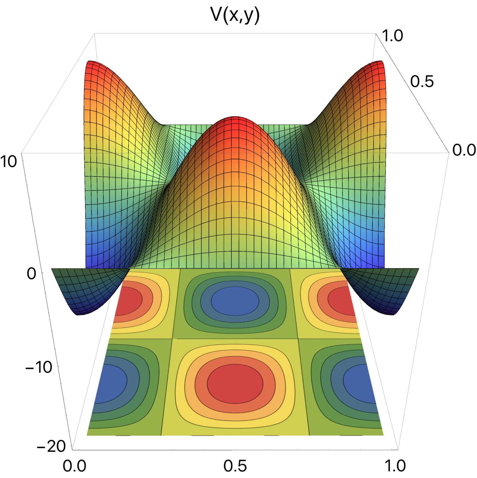
Refer to caption
(a) Potential VV
Refer to caption
(b) Density mm
Refer to caption
(c) Value function uu
Refer to caption
(d) Absolute numerical error
Fig. 6. Numerical solution of the variational problem (4.3) with N=50N=50 and for d=2d=2, P=(0,0)P=(0,0), V⁡(x,y)=10​sin⁡(2​π​(x+14))​cos⁡(2​π​(y+15))V(x,y)=10\sin\left(2\pi\left(x+\frac{1}{4}\right)\right)\cos\left(2\pi\left(y+\frac{1}{5}\right)\right), G⁡(m)=m22G(m)=\frac{m^{2}}{2}, α=1.5\alpha=1.5, and γ=2\gamma=2.
Refer to caption
(a) Potential VV
Refer to caption
(b) The density mm
Refer to caption
(c) The value function uu
Fig. 7. Numerical solution of the variational problem (4.3) with N=50N=50 and for d=2d=2, P=(1,3)P=(1,3), V⁡(x,y)=sin⁡(2​π​(x+14))​cos⁡(2​π​(y+14))V(x,y)=\sin\left(2\pi\left(x+\frac{1}{4}\right)\right)\cos\left(2\pi\left(y+\frac{1}{4}\right)\right), G⁡(m)=m3G(m)=m^{3}, α=1.5\alpha=1.5, and γ=2\gamma=2.
Grid size Max abs. error Mean abs. error Running time (s)
N=20N=20 0.03982920 0.011831300 3.39795
N=40N=40 0.00691211 0.002116950 222.576
N=80N=80 0.00108425 0.000318745 6032.06
Table 2. Numerical error and running time computation. Comparison between the closed-form solution, m¯​(x)=(V⁡(x)−H¯)+\bar{m}(x)=(V(x)-{\overline{H}})^{+}, where H¯∈ℝ{\overline{H}}\in{\mathbb{R}} is such that ∫𝕋2m¯​𝑑x=1\int_{{\mathbb{T}}^{2}}\bar{m}\,dx=1, and the numerical solution of the variational problem (4.3). Here, P=(0,0)P=(0,0), V⁡(x)=10​sin⁡(2​π​(x+14))​cos⁡(2​π​(y+14))V(x)=10\sin\left(2\pi\left(x+\frac{1}{4}\right)\right)\cos\left(2\pi\left(y+\frac{1}{4}\right)\right), G⁡(m)=m22G(m)=\frac{m^{2}}{2}, α=1.5\alpha=1.5, and γ=2\gamma=2.
Refer to caption
(a) Potential VV
Refer to caption
(b) Density mm
Refer to caption
(c) Value function uu
Fig. 8. Numerical solution of the variational problem (4.3) with N=50N=50 and for d=2d=2, P=(−1,3)P=(-1,3), V⁡(x,y)=e−sin⁡(2​π​(x+14))2​cos⁡(2​π​(y−14))V(x,y)=e^{-\sin\left(2\pi\left(x+\frac{1}{4}\right)\right)^{2}}\cos\left(2\pi\left(y-\frac{1}{4}\right)\right), G⁡(m)=m22+m3G(m)=\frac{m^{2}}{2}+m^{3}, α=2\alpha=2, and γ=2.5\gamma=2.5.

8. Numerical solution for the two-dimensional first-order MFGs with congestion, with 0<α<10<\alpha<1 and γ>1\gamma>1

In this section, we numerically solve the following MFG system, introduced in Section 5:

(8.1) {|P+D​u|γγ​mα+V⁡(x)−g⁡(m)=H¯in ​𝕋2div⁡(m1−α​|P+D​u|γ−2​(P+D​u))=0in ​𝕋2m>0,∫𝕋2m⁡(x)​dx=1\begin{cases}\frac{|P+Du|^{\gamma}}{\gamma m^{\alpha}}+V(x)-g(m)=\overline{H}&\quad\mbox{in }\;{\mathbb{T}}^{2}\\ \operatorname{div}(m^{1-\alpha}|P+Du|^{\gamma-2}(P+Du))=0&\quad\mbox{in }\;{\mathbb{T}}^{2}\\ m>0,\int_{{\mathbb{T}}^{2}}m(x)\,dx=1\end{cases}

for 0<α<10<\alpha<1 and γ>1\gamma>1. In the sequel, we describe a procedure to obtain a numerical solution of (8.1).

Step 1.

First, we define

γ′=γγ−1andα~=α−(α−1)​γ′.\gamma^{\prime}=\frac{\gamma}{\gamma-1}\quad\mbox{and}\quad\tilde{\alpha}=\alpha-(\alpha-1)\gamma^{\prime}.

Note that γ′>1\gamma^{\prime}>1 and 1<α~<γ′1<{\tilde{\alpha}}<\gamma^{\prime}.

Step 2.

Next, using the results from Section 5, we transform (8.1) into

(8.2) {|Q+D​ψ|γ′γ′​mα~+γγ′​V​(x)−γγ′​g​(m)=γγ′​H¯in ​𝕋2div⁡(m1−α~​|Q+D​ψ|γ′−2​(Q+D​ψ))=0in ​𝕋2m>0,∫𝕋2m(x)dx=1.\begin{cases}\frac{|Q+D\psi|^{\gamma^{\prime}}}{\gamma^{\prime}m^{{\tilde{\alpha}}}}+\frac{\gamma}{\gamma^{\prime}}V(x)-\frac{\gamma}{\gamma^{\prime}}g(m)={\frac{\gamma}{\gamma^{\prime}}}\overline{H}&\quad\mbox{in }\;{\mathbb{T}}^{2}\\ \operatorname{div}(m^{1-{\tilde{\alpha}}}|Q+D\psi|^{\gamma^{\prime}-2}(Q+D\psi))=0&\quad\mbox{in }\;{\mathbb{T}}^{2}\\ m>0,\int_{{\mathbb{T}}^{2}}m(x)\,dx=1.\end{cases}

Then, for each QQ, we solve the above system. For this, we formulate a variational principle analogous to (4.3). Namely, for fixed QQ, we minimize the functional

(8.3) J⁡[ψ,m]=∫𝕋2(|Q+D​ψ|γ′γ′​(α~−1)​mα~−1−γγ′​V​m+γγ′​G​(m))​𝑑xJ[\psi,m]=\int_{{\mathbb{T}}^{2}}\left(\frac{|Q+D\psi|^{\gamma^{\prime}}}{\gamma^{\prime}({\tilde{\alpha}}-1)m^{{\tilde{\alpha}}-1}}-\frac{\gamma}{\gamma^{\prime}}Vm+\frac{\gamma}{\gamma^{\prime}}G(m)\right)dx

under the constraints ∫𝕋2ψ​𝑑x=0\int_{{\mathbb{T}}^{2}}\psi\,dx=0, ∫𝕋dm​𝑑x=1\int_{{\mathbb{T}}^{d}}m\,dx=1, and m>0m>0, using the corresponding discretization for ψ\psi and mm. That is, considering the grid functions, ψ,m∈ℝN2\psi,m\in{\mathbb{R}}^{N^{2}}, we numerically solve

(8.4) min(ψ,m)∈𝒜h⁡Jh​[ψ,m],\min_{(\psi,m)\in\mathcal{A}_{h}}J_{h}[\psi,m],

where

(8.5) Jh​[ψ,m]=h2​∑i,j=0N−1((fh​([Dh​ψ],m))i,j−γγ′​Vi,j​mi,j+γγ′​G​(mi,j))J_{h}[\psi,m]=h^{2}\sum_{i,j=0}^{N-1}\left((f_{h}([D_{h}\psi],m))_{i,j}-\frac{\gamma}{\gamma^{\prime}}V_{i,j}m_{i,j}+\frac{\gamma}{\gamma^{\prime}}G(m_{i,j})\right)

with

(fh​([Dh​ψ],m))i,j=1mi,jα~−1​γ′​(α~−1)​((q1+(D1h​ψ)i,j)2+(q2+(D2h​ψ)i,j)2)γ′/2(f_{h}([D_{h}\psi],m))_{i,j}=\frac{1}{m_{i,j}^{{\tilde{\alpha}}-1}\gamma^{\prime}({\tilde{\alpha}}-1)}\left(\left(q_{1}+(D^{h}_{1}\psi)_{i,j}\right)^{2}+\left(q_{2}+(D^{h}_{2}\psi)_{i,j}\right)^{2}\right)^{\gamma^{\prime}/2}

for mi,j≠0m_{i,j}\not=0 and i,j∈{0,…,N−1}i,j\in\{0,\ldots,N-1\}. The set 𝒜h\mathcal{A}_{h} is the same as in (7.4), replacing uu by ψ\psi. Moreover, the discretization scheme is the one given in (7.1)–(7.2).

Step 3.

So far, for each QQ, we have ψ\psi and mm satisfying (8.4). Next, we determine the corresponding vector PP. By (5.2), we have

P⟂+(D​u)⟂=m1−α~​|Q+D​ψ|γ′−2​(Q+D​ψ).P^{\perp}+(Du)^{\perp}=m^{1-{\tilde{\alpha}}}|Q+D\psi|^{\gamma^{\prime}-2}(Q+D\psi).

Because uu is periodic, by integrating the previous expression in 𝕋2{\mathbb{T}}^{2}, we obtain

(8.6) P⟂=∫𝕋2m1−α~​|Q+D​ψ|γ′−2​(Q+D​ψ)​𝑑x.P^{\perp}=\int_{{\mathbb{T}}^{2}}m^{1-{\tilde{\alpha}}}|Q+D\psi|^{\gamma^{\prime}-2}(Q+D\psi)\,dx.

We observe that P⟂P^{\perp} can be obtained using the functional JJ. In fact, let

ϑ⁡[ψ,m]=|Q+D​ψ|γ′γ′​(α~−1)​mα~−1−γγ′​V​m+γγ′​G​(m)\vartheta[\psi,m]=\frac{|Q+D\psi|^{\gamma^{\prime}}}{\gamma^{\prime}({\tilde{\alpha}}-1)m^{{\tilde{\alpha}}-1}}-\frac{\gamma}{\gamma^{\prime}}Vm+\frac{\gamma}{\gamma^{\prime}}G(m)

denote the integrand of JJ. Taking the variational derivative of ϑ\vartheta with respect to mm in the direction of 11, we get

δδ​m​ϑ​[ψ,m]=limϵ→0ϑ⁡[ψ,m+ϵ]−ϑ⁡[ψ,m]ϵ=−|Q+D​ψ|γ′γ′​mα~−γγ′​V+γγ′​g​(m).\frac{\delta}{\delta m}\vartheta[\psi,m]=\lim_{\epsilon\to 0}\frac{\vartheta[\psi,m+\epsilon]-\vartheta[\psi,m]}{\epsilon}=-\frac{|Q+D\psi|^{\gamma^{\prime}}}{\gamma^{\prime}m^{{\tilde{\alpha}}}}-\frac{\gamma}{\gamma^{\prime}}V+\frac{\gamma}{\gamma^{\prime}}g(m).

Next, differentiating the expression above with respect to QQ, we obtain

−|Q+D​ψ|γ′−2​(Q+D​ψ)mα~.-\frac{|Q+D\psi|^{\gamma^{\prime}-2}(Q+D\psi)}{m^{{\tilde{\alpha}}}}.

Finally, multiplying this last expression by mm and integrating over 𝕋2{\mathbb{T}}^{2}, we obtain the right-hand side of (8.6). Therefore, P⟂P^{\perp} is alternatively given by

(8.7) P⟂=−∫𝕋2∂∂Q(δδ​mϑ[ψ,m](Q))mdx.\displaystyle P^{\perp}=-\int_{{\mathbb{T}}^{2}}\frac{\partial}{\partial Q}\left(\frac{\delta}{\delta m}\vartheta[\psi,m](Q)\right)m\,dx.

Recalling that P⟂=(−p2,p1)P^{\perp}=(-p_{2},p_{1}), we observe that the discrete version of (8.7) is

(8.8) p1=h2​∑i,j=0N−1(𝐃q2h​(𝐃mh​(ϑ⁡[ψ,m])​(q2))i,j​mi,j)i,j​d​xp2=−h2∑i,j=0N−1𝐃hq1(𝐃hm(ϑ[ψ,m])i,j(q1))i,jmi,jdx.\displaystyle\begin{split}p_{1}&=h^{2}\sum_{i,j=0}^{N-1}(\mathbf{D}^{h}_{q_{2}}(\mathbf{D}^{h}_{m}(\vartheta[\psi,m])(q_{2}))_{i,j}m_{i,j})_{i,j}\,dx\\ p_{2}&=-h^{2}\sum_{i,j=0}^{N-1}\mathbf{D}^{h}_{q_{1}}(\mathbf{D}^{h}_{m}(\vartheta[\psi,m])_{i,j}(q_{1}))_{i,j}m_{i,j}\,dx.\end{split}
Remark 8.1.

The notation (𝐃xh​(f⁡(x)))i,j(\mathbf{D}^{h}_{x}(f(x)))_{i,j} must be understood as the i,ji,j-node of the symbolic derivative of a grid function, ff, with respect to xx, whereas (𝐃fh​g​[f])i,j(\mathbf{D}_{f}^{h}g[f])_{i,j} is the symbolic variational derivative of gg with respect to ff in the direction of 11. In our implementation, we use symbolic calculus to compute those derivatives in a straightforward and automated fashion. Here, we obtain (8.8) using standard symbolic manipulations applied to JJ.

Step 4.

Finally, we use mm and PP from the previous steps and solve, for uu, the Hamilton–Jacobi equation,

(8.9) |P+D​u|γγ​mα+V⁡(x)−g⁡(m)=H¯in ​𝕋2.\frac{|P+Du|^{\gamma}}{\gamma m^{\alpha}}+V(x)-g(m)=\overline{H}\quad\mbox{in }\;{\mathbb{T}}^{2}.

Under the notation of Section 7.1, we use the following monotone scheme for |P+Dh​u|i,jγ|P+D^{h}u|_{i,j}^{\gamma}, i,j∈{0,…,N−1}i,j\in\{0,\ldots,N-1\}:

|P+Dh​u|i,jγ=\displaystyle|P+D^{h}u|_{i,j}^{\gamma}= max⁡(−p1−(D1h​u)i,j+,0)γ+max⁡(p1+(D1h​u)i−1,j+,0)γ\displaystyle\max(-p_{1}-(D^{h}_{1}u)^{+}_{i,j},0)^{\gamma}+\max(p_{1}+(D^{h}_{1}u)^{+}_{i-1,j},0)^{\gamma}
+max⁡(−p2−(D2h​u)i,j+,0)γ+max⁡(p2+(D2h​u)i,j−1+,0)γ.\displaystyle+\max(-p_{2}-(D^{h}_{2}u)^{+}_{i,j},0)^{\gamma}+\max(p_{2}+(D^{h}_{2}u)^{+}_{i,j-1},0)^{\gamma}.

From [32], we have that

β​u(β)+|P+D​u(β)|γγ​mα+V⁡(x)−g⁡(m)=0in ​𝕋2\beta u^{(\beta)}+\frac{|P+Du^{(\beta)}|^{\gamma}}{\gamma m^{\alpha}}+V(x)-g(m)=0\quad\mbox{in }\;{\mathbb{T}}^{2}

converges to (8.9) when β→0\beta\to 0; that is, β​u(β)\beta u^{(\beta)} converges uniformly to −H¯-{\overline{H}}, and u(β)−maxx∈𝕋2⁡u⁡(x)u^{(\beta)}-\max_{x\in{\mathbb{T}}^{2}}u(x) converges uniformly, up to subsequences, to uu. We then use the notation for grid functions from Section 7.1, and numerically solve, for small β>0\beta>0, the discrete problem

β​ui,j(β)+|Dh​u(β)+P|i,jγγ​mi,jα+Vi,j−gi,j=0in 𝕋N2.\beta u^{(\beta)}_{i,j}+\frac{|D^{h}u^{(\beta)}+P|_{i,j}^{\gamma}}{\gamma m^{\alpha}_{i,j}}+V_{i,j}-g_{i,j}=0\quad\mbox{in ${\mathbb{T}}^{2}_{N}$}.

Hence, we set

H¯(β)=max⁡{ui,j(β),i,j∈{0,…,N−1}}.\overline{H}^{(\beta)}=\max\{u^{(\beta)}_{i,j},\;i,j\in\{0,\ldots,N-1\}\}.

Finally, the solution of (8.9) is approximated by

ui,j≅ui,jβ−H¯β.u_{i,j}\cong u^{\beta}_{i,j}-\overline{H}^{\beta}.

8.1. Numerical experiments

In Fig. 9, we illustrate the solution of (8.1) for α=0.8\alpha=0.8, γ=2\gamma=2, and P=(1,3)P=(1,3). Moreover, we use the coupling G⁡(m)=m3G(m)=m^{3} and the potential

V⁡(x,y)=sin⁡(2​π​(x+14))​cos⁡(2​π​(y+14)).V(x,y)=\sin\left(2\pi\left(x+\frac{1}{4}\right)\right)\cos\left(2\pi\left(y+\frac{1}{4}\right)\right).

In this example, we have Q=(3,−1)Q=(3,-1). The value function, uu, and the density, mm, are displayed in Figs. 9(c) and 9(b), respectively. Note that, even with α<1\alpha<1, the density is similar to the density in Fig. 7(b). However, for this example, the value function behaves differently from what we observed in Fig. 7(c).

Refer to caption
(a) Potential VV
Refer to caption
(b) Density mm
Refer to caption
(c) Value function uu
Fig. 9. Numerical solution of (8.1) with N=50N=50 and for P=(1,3)P=(1,3), V⁡(x,y)=sin⁡(2​π​(x+14))​cos⁡(2​π​(y+14))V(x,y)=\sin\left(2\pi\left(x+\frac{1}{4}\right)\right)\cos\left(2\pi\left(y+\frac{1}{4}\right)\right), G⁡(m)=m3G(m)=m^{3}, α=0.8\alpha=0.8, and γ=2\gamma=2.

9. Numerical solution for the second-order MFGs with congestion, with γ=2\gamma=2 and 1<α<γ1<\alpha<\gamma

In this section, for illustration purposes, we numerically solve a variational problem introduced in Section 6.2, which corresponds to a second-order MFG with congestion in the quadratic case. More precisely, we consider the minimization problem

(9.1) minψ⩾0⁡J^​[ψ],J^​[ψ]=∫𝕋d[|D​ψ|22​α+1+G^​(ψ)−2​α+12​(α+1)​(V⁡(x)−H¯)​ψ2​(α+1)2​α+1]​𝑑x,\min_{\psi\geqslant 0}\hat{J}[\psi],\quad\hat{J}[\psi]=\int_{{\mathbb{T}}^{d}}\bigg[\frac{|D\psi|^{2}}{2\alpha+1}+\hat{G}(\psi)-\frac{2\alpha+1}{2(\alpha+1)}(V(x)-\overline{H})\psi^{\frac{2(\alpha+1)}{2\alpha+1}}\bigg]dx,

where, for z⩾0z\geqslant 0,

(9.2) G^​(z)=∫0zg⁡(r22​α+1)​r12​α+1​𝑑r\hat{G}(z)=\int_{0}^{z}g(r^{\frac{2}{2\alpha+1}})r^{\frac{1}{2\alpha+1}}\,dr

and H¯{\overline{H}} is chosen such that the constraint

(9.3) ∫𝕋dψ22​α+1​dx=1\displaystyle\int_{{\mathbb{T}}^{d}}\psi^{\frac{2}{2\alpha+1}}\,dx=1

holds. Recall that the Euler–Lagrange equation of the functional in (9.1) is (6.10). Moreover, (6.10) corresponds to (6.9) for γ=2\gamma=2.

Using the notation for grid functions introduced in Section 7.1, we present the discretized version of (9.1) in the two-dimensional case as follows. For a grid function, ψ∈ℝN2\psi\in{\mathbb{R}}^{N^{2}}, we numerically solve

(9.4) minψ⩾0⁡Jh​[ψ],\min_{\psi\geqslant 0}J_{h}[\psi],

where

Jh​[ψ]=h2​∑i,j=0N−1((fh​([Dh​ψ]))i,j+G⁡(ψi,j)−2​α+12​(α+1)​(Vi,j−H¯)​ψi,j2​(α+1)2​α+1)J_{h}[\psi]=h^{2}\sum_{i,j=0}^{N-1}\left((f_{h}([D_{h}\psi]))_{i,j}+G(\psi_{i,j})-\frac{2\alpha+1}{2(\alpha+1)}(V_{i,j}-\overline{H})\psi_{i,j}^{\frac{2(\alpha+1)}{2\alpha+1}}\right)

and

(fh​([Dh​ψ]))i,j=1(2​α+1)​(((D1h​ψ)i,j)2+((D2h​ψ)i,j)2).(f_{h}([D_{h}\psi]))_{i,j}=\frac{1}{(2\alpha+1)}\left(\left((D^{h}_{1}\psi)_{i,j}\right)^{2}+\left((D^{h}_{2}\psi)_{i,j}\right)^{2}\right).

Moreover, as in the previous sections, the discretization scheme follows (7.1)–(7.2). Recall that P=(0,0)P=(0,0) here. In the following subsection, we perform a numerical experiment to illustrate our method.

9.1. Numerical experiment in the two-dimensional case

Here, we depict a numerical solution of (9.1) for the potential

V⁡(x,y)=e−sin⁡(2​π​(x+14))2​sin⁡(2​π​(y−14)),V(x,y)=e^{-\sin\left(2\pi\left(x+\frac{1}{4}\right)\right)^{2}}\sin\left(2\pi\left(y-\frac{1}{4}\right)\right),

the coupling g⁡(r)=r3g(r)=r^{3} (see (9.2)), and α=1.5\alpha=1.5 (see Fig. 10). For this example, the value of H¯\overline{H} such that (9.3) is satisfied is approximately H¯≅−3.001\overline{H}\cong-3.001. The density, mm, is displayed in Fig. 10(b). In this example, we note that the density still resembles the potential. However, diffusion tends to spread the distribution of the agents making it more uniform.

Refer to caption
(a) Potential VV
Refer to caption
(b) Density mm
Fig. 10. Numerical solution of (9.1) with N=50N=50 and for d=2d=2, V⁡(x,y)=e−sin⁡(2​π​(x+14))2​sin⁡(2​π​(y−14))V(x,y)=e^{-\sin\left(2\pi\left(x+\frac{1}{4}\right)\right)^{2}}\sin\left(2\pi\left(y-\frac{1}{4}\right)\right), g⁡(m)=m3g(m)=m^{3}, and α=1.5\alpha=1.5.

10. Conclusions

In this paper, we develop a new variational formulation for systems of first-order MFGs with congestion. This variational principle provides a new construction of weak solutions and leads to a novel numerical approach through an optimization problem.

Even though the variational structure strongly depends on the form of the MFGs, it is often possible to modify the variational principle. This approach was followed in Section 5 for the first-order case and in Section 6 for the second-order case. Moreover, in Sections 7–9, we use these results to obtain new numerical solutions for MFGs with congestion.

References

  • [1] Y. Achdou and A. Porretta. Mean field games with congestion. ArXiv preprint, 2016. arXiv:1706.08252 [math.AP].
  • [2] N. Al-Mulla, R. Ferreira, and D. Gomes. Two numerical approaches to stationary mean-field games. To appear Dyn. Games and Appl., 2016.
  • [3] Jean-David Benamou, Guillaume Carlier, and Filippo Santambrogio. Variational mean field games. In Active particles. Vol. 1. Advances in theory, models, and applications, Model. Simul. Sci. Eng. Technol., pages 141–171. Birkhäuser/Springer, Cham, 2017.
  • [4] L. Boccardo, L. Orsina, and A. Porretta. Strongly coupled elliptic equations related to mean-field games systems. J. Differential Equations, 261(3):1796–1834, 2016.
  • [5] P. Cardaliaguet and P. J. Graber. Mean field games systems of first order. ESAIM Control Optim. Calc. Var., 21(3):690–722, 2015.
  • [6] Pierre Cardaliaguet, Alpár R. Mészáros, and Filippo Santambrogio. First order mean field games with density constraints: pressure equals price. SIAM J. Control Optim., 54(5):2672–2709, 2016.
  • [7] M. Cirant. A generalization of the Hopf–Cole transformation for stationary Mean-Field Games systems. C. R. Math. Acad. Sci. Paris, 353(9):807–811, 2015.
  • [8] B. Dacorogna and P. Maréchal. The role of perspective functions in convexity, polyconvexity, rank-one convexity and separate convexity. J. Convex Anal., 15(2):271–284, 2008.
  • [9] D. Evangelista and D. Gomes.
  • [10] D. Evangelista, D. Gomes, and L. Nurbekyan. Radially symmetric mean-field-games with congestion. ArXiv preprint, 2017. arXiv:1703.07594v1 [math.AP].
  • [11] R. Ferreira and D. Gomes. Existence of weak solutions for stationary mean-field games through variational inequalities. Preprint, 2016.
  • [12] Irene Fonseca and Giovanni Leoni. Modern methods in the calculus of variations: LpL^{p} spaces. Springer Monographs in Mathematics. Springer, New York, 2007.
  • [13] D. Gomes and H. Mitake. Existence for stationary mean-field games with congestion and quadratic Hamiltonians. NoDEA Nonlinear Differential Equations Appl., 22(6):1897–1910, 2015.
  • [14] D. Gomes, L. Nurbekyan, and M. Prazeres. Explicit solutions of one-dimensional, first-order, stationary mean-field games with congestion. 2016 IEEE 55th Conference on Decision and Control, CDC 2016, pages 4534–4539, 2016.
  • [15] D. Gomes, L. Nurbekyan, and M. Prazeres. One-dimensional stationary mean-field games with local coupling. Dyn. Games and Applications, 2017.
  • [16] D. Gomes, S. Patrizi, and V. Voskanyan. On the existence of classical solutions for stationary extended mean field games. Nonlinear Anal., 99:49–79, 2014.
  • [17] D. Gomes, E. Pimentel, and V. Voskanyan. Regularity theory for mean-field game systems. SpringerBriefs in Mathematics. Springer, [Cham], 2016.
  • [18] D. Gomes, G. E. Pires, and H. Sánchez-Morgado. A-priori estimates for stationary mean-field games. Netw. Heterog. Media, 7(2):303–314, 2012.
  • [19] D. Gomes and R. Ribeiro. Mean field games with logistic population dynamics. 52nd IEEE Conference on Decision and Control (Florence, December 2013), 2013.
  • [20] D. Gomes and H. Sánchez Morgado. A stochastic Evans-Aronsson problem. Trans. Amer. Math. Soc., 366(2):903–929, 2014.
  • [21] D. Gomes and J. Saúde. Numerical methods for finite state mean-field games that satisfy a monotonicity condition. Preprint, 2017.
  • [22] D. Gomes and V. Voskanyan. Short-time existence of solutions for mean-field games with congestion. J. Lond. Math. Soc. (2), 92(3):778–799, 2015.
  • [23] J. Graber. Weak solutions for mean field games with congestion. Preprint, 2015.
  • [24] O. Guéant. A reference case for mean field games models. J. Math. Pures Appl. (9), 92(3):276–294, 2009.
  • [25] O. Guéant. New numerical methods for mean field games with quadratic costs. Netw. Heterog. Media, 7(2):315–336, 2012.
  • [26] M. Huang, P. E. Caines, and R. P. Malhamé. Large-population cost-coupled LQG problems with nonuniform agents: individual-mass behavior and decentralized ϵ\epsilon-Nash equilibria. IEEE Trans. Automat. Control, 52(9):1560–1571, 2007.
  • [27] M. Huang, R. P. Malhamé, and P. E. Caines. Large population stochastic dynamic games: closed-loop McKean-Vlasov systems and the Nash certainty equivalence principle. Commun. Inf. Syst., 6(3):221–251, 2006.
  • [28] J.-M. Lasry and P.-L. Lions. Jeux à champ moyen. I. Le cas stationnaire. C. R. Math. Acad. Sci. Paris, 343(9):619–625, 2006.
  • [29] J.-M. Lasry and P.-L. Lions. Jeux à champ moyen. II. Horizon fini et contrôle optimal. C. R. Math. Acad. Sci. Paris, 343(10):679–684, 2006.
  • [30] J.-M. Lasry and P.-L. Lions. Mean field games. Jpn. J. Math., 2(1):229–260, 2007.
  • [31] P.-L. Lions. Collége de France course on mean-field games. 2007-2011.
  • [32] P. L. Lions, G. Papanicolao, and S. R. S. Varadhan. Homogeneization of Hamilton-Jacobi equations. Preliminary Version, 1988.
  • [33] L. Nurbekyan. One-dimensional, non-local, first-order, stationary mean-field games with congestion: a Fourier approach. To appear in DCDS - series S, 2017. arXiv:1703.03954v1 [math.AP].
  • [34] E. Pimentel and V. Voskanyan. Regularity for second-order stationary mean-field games. Indiana Univ. Math. J., 66(1):1–22, 2017.
  • [35] F. Santambrogio. A modest proposal for MFG with density constraints. Netw. Heterog. Media, 7(2):337–347, 2012.
  • [36] Huibing Yin, Prashant G. Mehta, Sean P. Meyn, and Uday V. Shanbhag. On the efficiency of equilibria in mean-field oscillator games. Dyn. Games Appl., 4(2):177–207, 2014.