Image Labeling Based on Graphical Models
Using Wasserstein Messages and Geometric AssignmentThanks: Support by the German Science Foundation, grant GRK 1653, is gratefully acknowledged.
Abstract.
We introduce a novel approach to Maximum A Posteriori inference based on discrete graphical models. By utilizing local Wasserstein distances for coupling assignment measures across edges of the underlying graph, a given discrete objective function is smoothly approximated and restricted to the assignment manifold. A corresponding multiplicative update scheme combines in a single process (i) geometric integration of the resulting Riemannian gradient flow and (ii) rounding to integral solutions that represent valid labelings. Throughout this process, local marginalization constraints known from the established LP relaxation are satisfied, whereas the smooth geometric setting results in rapidly converging iterations that can be carried out in parallel for every edge.
Key words and phrases:
image labeling, assignment manifold, Fisher–Rao metric, Riemannian gradient flow, discrete optimal transport, Wasserstein distance, entropic regularization, graphical models2010 Mathematics Subject Classification
62H35, 62M40, 65K10, 68U101. Introduction
1.1. Overview and Motivation
Let be a domain where image data are observed, and let , denote a grid graph embedded into . Each vertex indexes the location of a pixel, to which a random variable
| (1.1) |
is assigned which takes values in a finite set of labels. The image labeling problem is the task to assign to each a label such that the discrete objective function
| (1.2) |
is minimized. This function comprises for each pixel local energy terms that evaluate local label predictions for each possible value of . In addition, comprises for each edge local distance functions that evaluate the joint assignment of labels to and . If the local energy functions are defined by a metric , then (1.2) is called the metric labeling problem [KT02]. In general, the presence of these latter terms makes image labeling a combinatorially hard task. Function has the common format of variational problems for image analysis comprising a data term and a regularizer. From a Bayesian perspective, therefore, minimizing corresponds to Maximum A-Posteriori inference with respect to the probability distribution . We refer to [KAH+15] for a recent survey on the image labeling problem and on algorithms for solving either approximately or exactly problem (1.2).
A major class of algorithms for approximately solving (1.2) is based on the linear (programming) relaxation [Wer07] (see Section 2.2 for details)
| (1.3) |
Solving the linear program (LP) (1.3) returns a globally optimal relaxed indicator vector whose components take values in . If is a binary vector, then it corresponds to a solution of problem (1.2). In realistic applications, this is not the case, however, and the relaxed solution has to be rounded to an integral solution in a post-processing step.
In this paper, we present an alternative inference algorithm that deviates from the traditional two-step process: convex relaxation and rounding. It is based on the recently proposed geometric approach [ÅPSS17] to image labeling. The basic idea underlying this approach is to restrict indicator vector fields to the relative interior of the probability simplex, equipped with the Fisher-Rao metric, and to regularize label assignments by iteratively computing Riemannian means (see Section 3 for details). This results in a highly parallel, multiplicative update scheme, that rapidly converges to an integral solution. Because this model of label assignment does not interfere with data representation, the approach applies to any data given in a metric space. The recent paper [BFPS17] reports a convergence analysis and the application of our scheme to a range of challenging labeling problems of manifold-valued data.
Adopting this starting point, the objectives of the present paper are:
- •
- •
Devise a novel labeling algorithm that tightly integrates both relaxation and rounding to an integral solution in a single process.
- •
Stick to the smooth geometric model suggested by [ÅPSS17] so as to overcome the inherent non-smoothness of convex polyhedral relaxations and the slow convergence of corresponding first-order iterative methods of convex programming.
Regarding the last point, a key ingredient of our approach is a smooth approximation
| (1.4) |
of problem (1.3), where denotes the local smoothed Wasserstein distance between the discrete label assignment measures coupled along the edge of the underlying graph. Besides achieving the degree of smoothness required for our geometric setting, this approximation also properly takes into account the regularization parameters that are specified in terms of the local energy terms of the labeling problem (1.2). Our approach restricts the function to the so-called assignment manifold and iteratively determines a labeling by tightly combining geometric optimization with rounding to an integral solution in a smooth fashion.
1.2. Related Work
Problem sizes of linear program (LP) (1.3) are large in typical applications of image labeling, which rules out the use of standard LP codes. In particular, the theoretically and practically most efficient interior point methods based on self-concordant barrier functions [NN87, Ren95] are infeasible due to the dense linear algebra steps required to determine search and update directions.
Therefore, the need for dedicated solvers for the LP relaxation (1.3) has stimulated a lot of research. A prominent example constitute subclasses of objective functions (1.2) as studied in [KZ04], in particular binary submodular functions, that enable to reformulate the labeling problem as maximum-flow problem in an associated network and the application of discrete combinatorial solvers [BVZ01, BK04].
Since the structure of such algorithms inherently limits fine-grained parallel implementations, however, belief propagation and variants [YFW05] have been popular among practitioners. These fixed point schemes in terms of dual variables iteratively enforce the so-called local polytope constraints that define the feasible set of the LP relaxation (1.3). They can be efficiently implemented using ‘message passing’ and exploit the structure of the underlying graph. Although convergence is not guaranteed on cyclic graphs, the performance in practice may be good [YMW06]. The theoretical deficiencies of basic belief propagation in turn stimulated research on convergent message passing schemes, either using heuristic damping or utilizing in a more principled way convexity. Prominent examples of the latter case are [WJW05, HS10]. We refer to [KAH+15] for many more references and a comprehensive experimental evaluation of a broad range of algorithms for image labeling.
The feasible set of the relaxation (1.3) is a superset of the original feasible set of (1.2). Therefore, globally optimal solutions to (1.3) generally do not constitute valid labelings but comprise non-integral components . Randomized rounding schemes for converting a relaxed solution vector to a valid labeling , along with suboptimality bounds, were studied in [KT02, CKNZ05]. The problem to infer components of the unknown globally optimal combinatorial labeling that minimizes (1.2), through partial optimality and persistency, was studied in [SSK+16]. We refer to [Wer07] for the history and more information about the LP relaxation of labeling problems, and to [WJ08] for connections to discrete probabilistic graphical models from the variational viewpoint.
The approach [RAW10] applies the mirror descent scheme [NY83] to the LP (1.3). This amounts to sequential proximal minimization [Roc76], yet using a Bregman distance as proximity measure instead of the squared Euclidean distance [CZ92]. A key technical aspect concerns the proper choice of entropy functions related to the underlying graphical model, that qualify as convex functions of Legendre type (cf. [BB97]). The authors of [RAW10] observed a fast convergence rate. However, the scheme does not scale up to the typically large problem sizes used in image analysis, especially when graphical models with higher edge connectivity are considered, due to the memory requirements when working entirely in the primal domain.
Optimal transport and the Wasserstein distance have become a major tool of signal modeling and analysis [KPT+17]. In connection with the metric labeling problem, using the Wasserstein distance (aka. optimal transport costs, earthmover metrics) was proposed before by [AFH+04] and [CKNZ05]. These works study bounds on the integrality gap of an ‘earthmover LP’ and performance guarantees of rounding procedures applied as post-processing. While the earthmover LP corresponds to our approach (1.4) without smoothing, authors do not specify how to solve such LPs efficiently, especially when the LP relates to a large-scale graphical models as in image analysis. Moreover, the bounds derived by [AFH+04] become weak with increasing numbers of variables, which are fairly large in typical problems of image analysis. In contrast, the focus of the present paper is on a smooth geometric problem reformulation that scales well with both the problem size and the number of labels, and performs rounding simultaneously. If and how theoretical guarantees regarding the integrality gap and rounding carry over to our setting, is an interesting open research problem of future research.
Regarding the finite-dimensional formulation of optimal discrete transport in terms of linear programs, the design of efficient algorithms for large-scale problems requires sophisticated techniques [Sch16a]. The problems of discrete optimal transport studied in this paper, in connection with the local Wasserstein distances of (1.4), have a small or moderate size (: number of labels squared). We apply the standard device of enhancing convexity through entropic regularization, which increases smoothness in the dual domain. We refer to [Sch90] and [Bru06, Ch. 9] for basic related work and the connection to matrix scaling algorithms and the history. When entropic regularization is very weak and for large problem sizes, the related fixed point iteration suffers from numerical instability, and dedicated methods for handling them have been proposed [Sch16b]. Smoothing of the Wasserstein distance and Sinkhorn’s algorithm has become popular in machine learning due to [Cut13]. The authors of [Pey15, CP16] comprehensively investigated barycenters and interpolation based on the Wasserstein distance. Our approach to image labeling, in conjunction with the geometric approach of [ÅPSS17], is novel and elaborates [ÅHS+17].
Finally, since our approach is defined on a graph and works with data on a graph, our work may be assigned to the broad class of nonlocal methods for image analysis on graphs, from a more general viewpoint. Recent major related work includes [BF12] on the connection between the Ginzburg-Landau functional for binary regularized segmentation and spectral clustering, and [BT17] on generalizing PDE-like models on graphs to manifold-valued data. We refer to the bibliography in these works and to the seminal papers [Amb89] on regularized variational segmentation using -convergence and to [GO08, ELB08] on nonlocal variational image processing on graphs, that initiated these fast evolving lines of research. The focus on the present paper however is on discrete graphical models and the corresponding labeling problem, in terms of any discrete objective function of the form (1.2).
1.3. Contribution and Organization
We collect basic notation, background material and details of the LP relaxation (1.3) in Section 2. Section 3 summarizes the basic concepts of the geometric labeling approach of [ÅPSS17], in particular the so-called assignment manifold, and the general framework of [SHÅ+17] for numerically integrating Riemannian gradient flows of functionals defined on the assignment manifold. This section provides the basis for the two subsequent sections that contain our main contribution.
Section 4 studies the approximation (1.4) and provides explicit expressions for the Riemannian gradient of the restriction of to the assignment manifold. A key property of this set-up concerns the local polytope constraints that define the feasible set of the LP relaxation (1.3): by construction, they are always satisfied throughout the resulting iterative process of label assignment. Thus, our formulation is both more tightly constrained and smooth, in contrast to the established convex programming approaches based on (1.3).
Section 5 details the combination of all ingredients into a single, smooth, geometric approach that performs simultaneously minimization of the objective function (1.4) and rounding to an integral solution (label assignment). This tight integration is a second major property that distinguishes our approach from related work. Section 5 also explains the notion ‘Wasserstein messages’ in the title of this paper due to the dual variables that are numerically utilized to evaluate gradients of local Wasserstein distances, akin to how dual (multiplier) variables in basic belief propagation schemes are used to enforce local marginalization constraints. Unlike the latter computations they have the structure of message passing on a dataflow architecture, however, message passing induced by our approach is fully parallel along all edges of the underlying graph and hence resembles the structure of numerical solvers for PDEs.
The remaining two sections are devoted to numerical evaluations of our approach. To keep this paper at a reasonable length, we merely consider the most elementary iterative update scheme, based on the geometric integration of the Riemannian gradient flow with the (geometric) explicit Euler scheme. The potential of the framework outlined by [SHÅ+17] for more sophisticated numerical schemes will be explored elsewhere along with establishing bounds for parameter values that provably ensure stability of numerical integration of the underlying gradient flow. Furthermore, working out any realistic application is beyond the scope of this paper. Rather, the experimental results demonstrate major properties of our approach.
Section 6 provides all details of our implementation that are required to reproduce our computational results. Section 7 reports and discusses the results of four types of experiments:
- (1)
The interplay between two parameters and that control smoothness of the approximation (1.4) and rounding, respectively, is studied. In order to miminize efficiently (1.2), the Riemannian flow with respect to the smooth approximation (1.4) must reveal proper descent directions. This imposes an upper bound on the smoothing parameter . Naturally, the effect of rounding has to be stronger to make the iterative process converge to an integral solution. A corresponding choice of controls the compromise between quality of integral labelings in terms of the energy (1.4) and speed of convergence. Fortunately, the upper bound on is large enough to achieve attractive convergence rates.
- (2)
We comprehensively explore numerically the entire model space of the minimal binary graphical model on the cyclic triangle graph , whose relaxation in terms of the so-called local polytope already constitutes a superset of the marginal polytope as admissible set for valid integral labelings. In this way, we explore the performance of our approach in view of the LP relaxation and established inference based on convex programming, and with respect to the (generally intractable) feasible set of integral solutions. Corresponding phase diagrams display and support quantitatively the trade-off between accuracy of optimization and rate of convergence through the choice of the single parameter .
- (3)
A labeling problem of the usual size was conducted to confirm and demonstrate that the finding of the preceding points for ‘all’ models on also hold in a typical application. A comparison to sequential tree-reweighted message passing (TRWS) [Kol06] which defines the state of the art, and to loopy belief propagation (BP) based on the OpenGM package [ABK12], shows that our approach is on par with these methods regarding the energy level of the resulting labeling .
- (4)
A final experiment based on the graphical model with a pronounced non-uniform (non-Potts) prior demonstrates that our approach is able to perform inference for any given graphical model.
We conclude in Section 8 and relegate some proofs to an Appendix in order not to interrupt too much the overall line of reasoning.
2. Preliminaries
We introduce basic notation in Section 2.1 and the common linear programming (LP) relaxation of the labeling problem in Section 2.2. In order to clearly distinguish between the LP relaxation and our geometric approach to the labeling problem based on [ÅPSS17] (see Section 3.1), we keep the standard notation in the literature for the former approach and the notation from [ÅPSS17] for the latter one. Remark 3.1 below identifies variables of both approaches that play a similar role.
2.1. Basic Notation
For an undirected graph , the adjacency relation means that vertices and are connected by an undirected edge , where the latter denotes the unordered pair . The neighbors of vertex form the set
| (2.1) |
of all vertices adjacent to , and its cardinality is the degree of . is turned into a directed graph by assigning an orientation to every edge , which then form ordered pairs denoted by . We only consider graphs without multiple edges between any pair of nodes .
We use the abbreviation for . denotes the extended real line. All vectors are regarded as column vectors, and denotes transposition of a vector . We ignore transposition however when vectors are explicitly specified by their components; e.g. we write instead of the more cumbersome . We set and write if is clear from the context. denotes the Euclidean inner product. Given a matrix
| (2.2) |
we denote the row vectors by and the column vectors by . The canonical matrix inner product is , where denotes the trace of a matrix, i.e. . Superscripts in brackets, e.g. , index iterative steps.
The set of nonnegative vectors is denoted by and the set of strictly positive vectors by . The probability simplex contains all discrete distributions on . A doubly stochastic matrix , also called coupling measure in this paper in connection with discrete optimal transport, has the property: and . We denote these two marginal distributions of by and , respectively, and the linear mapping for extracting them by
| (2.3a) | ||||
| Its transpose is given by | ||||
| (2.3b) | ||||
The kernel (nullspace) of a linear mapping is denoted by and its range by .
The functions apply componentwise to strictly positive vectors , e.g. , and similarly for strictly positive matrices. Likewise, if , then we simply write
| (2.4) |
for the componentwise multiplication and division.
We define to be the class of proper, lower-semicontinuous and convex functions defined on . For any function , denotes its subdifferential at , and the conjugate function of is given by the Legendre-Fenchel transform (cf. [RW09, Section 11.A])
| (2.5) |
For a given closed convex set , its indicator function is denoted by
| (2.6) |
and
| (2.7) |
denotes the orthogonal projection onto . The shorthand “s.t.” means: “subject to” in connection to the specification of constraints.
The log-exponential function is defined as
| (2.8a) | ||||
| It uniformly approximates the function [RW09, Ex. 1.30], i.e. | ||||
| (2.8b) | ||||
We will use the following basic result from convex analysis (cf., e.g. [RW09, Ch. 11]), where denotes the subdifferential of a function at .
Theorem 2.1 (inversion rule for subgradients).
Let . Then
| (2.9) |
We will also apply the following classical theorem of Danskin and its extension by Rockafellar.
2.2. The Local Polytope Relaxation of the Labeling Problem
We sketch in this section the transition from the discrete energy minimization problem (1.2) to the LP relaxation (1.3) and thereby introduce additional notation needed in subsequent sections.
The first step concerns the definition of local model parameter vectors and matrices
| (2.11) |
which merely encode the values of the discrete objective function (1.2): , . These local terms are commonly called unary and pairwise terms in the literature. Recall from the discussion of (1.2) that the unary terms represent the data and the pairwise terms specify a regularizer. All these local terms are indexed by the vertices and edges of the underlying graph and assembled into the vectors
| (2.12) |
where we conveniently regard either as local vector or as local matrix , depending on the context. Next we define local indicator vectors
| (2.13) |
indexed in the same way as (2.11) and assembled into the vectors
| (2.14) |
The combinatorial optimization problem (1.2) now reads . The corresponding linear programming relaxation consists in replacing the discrete feasible set of (2.13) by the convex polyhedral sets
| (2.15a) | ||||
| (2.15b) | ||||
As a result, the linear programming relaxation (1.3) of (1.2) reads more explicitly
| (2.16) |
where the so-called local polytope is the set of all vectors of the form (2.14) with components ranging over the sets specified by (2.15). The adjective “local” refers to the local marginalization constraints (2.15b).
3. Image Labeling on the Assignment Manifold
This section sets the stage for our approach to solving approximately the labeling problem (1.2). We first introduce in Section 3.1 in terms of the assignment manifold the setting for the smooth approach to image labeling [ÅPSS17], to be sketched in Section 3.2. Section 3.3 summarizes the general framework of [SHÅ+17] for numerically integrating Riemannian gradient flows of functionals defined on the assignment manifold.
3.1. The Assignment Manifold
The relative interior of the probability simplex , given by , is a dimensional smooth manifold with constant tangent space
| (3.1) |
Due to for all , we have the orthogonal decomposition . The orthogonal projection onto is given by
| (3.2) |
where denotes the identity matrix. The manifold becomes a Riemannian manifold by endowing it with the Fisher-Rao metric. At a point , this metric is given by
| (3.3) |
In this setting, there is an important map, called the lifting map (cf. [ÅPSS17, Def. 4]), defined as
| (3.4) |
By restricting onto the tangent space, we obtain a diffeomorphism
| (3.5) |
This restricted lifting map is also a local first order approximation to the exponential map of the Riemannian manifold (cf [ÅPSS17, Prop. 3]), with the inverse mapping given by
| (3.6) |
The assignment manifold is defined as the product manifold and can be identified with the space of row-stochastic matrices with full support. With the Riemannian product metric, also becomes a Riemannian manifold with constant tangent space
| (3.7) |
The Fisher-Rao product metric reads
| (3.8) |
The orthogonal decomposition of induces the orthogonal decomposition
| (3.9) |
together with the orthogonal projection
| (3.10) |
Thus, the projection of a matrix onto is just the projection (3.2) applied to every row of . The lifting map, the restricted lifting map and its inverse are naturally extended to
| (3.11) |
for every , by applying , and from (3.4), (3.5), (3.6) to every row,
| (3.12) |
for , , and .
3.2. Image Labeling on
In [ÅPSS17] the following approach was proposed. Let be a graph with vertex set . Suppose a function is given on this graph with values in some feature space ,
| (3.13) |
Furthermore, let the set from (1.1) denote a set of prototypes or labels (possibly ) and assume a distance function is specified,
| (3.14) |
measuring how well a feature is represented by a certain prototype. We are interested in the assignment of the prototypes to the data in terms of an assignment matrix . The elements of can be interpreted as the posterior probability
| (3.15) |
that generated the observation . The assignment task of determining an optimal assignment can thus be interpreted as finding an ‘explanation’ of the data in terms of the prototypes .
Remark 3.1 ( vs. ).
The objective function for measuring the quality of an assignment involves three matrices defined next. First, all distance information between observed feature vectors and prototypes (labels) are gathered by the distance matrix
| (3.16) |
and then lifted onto the assignment manifold at . By using (3.11) we obtain the likelihood matrix
| (3.17) |
where each row of is given by and is given by (3.10). Finally, the similarity matrix
| (3.18) |
is defined as a local geometric average of assignment vectors at neighboring nodes, i.e. the -th row is defined to be the Riemannian mean (cf. [ÅPSS17, Def. 2])
| (3.19) |
of the lifted distances in the neighborhood .
The correlation between and the local averages defining , as measured by the basic matrix inner product, is used as the objective function
| (3.20) |
to be maximized. The optimization strategy is to follow the Riemannian gradient ascent flow on (see Section 3.3 for the formal definition of the Riemannian gradient)
| (3.21) |
The initialization with the barycenter of constitutes an uninformative uniform assignment which is not biased towards any prototype.
To obtain an efficient numerical algorithm, the Riemannian mean is approximated using the geometric mean
| (3.22) |
Based on the simplifying, plausible assumption that the mean only changes slowly and by using the explicit Euler-method directly on with a certain adaptive step-size (cf. [ÅPSS17, Sect. 3.3]), the following multiplicative update scheme is obtained
| (3.23) |
3.3. Geometric Integration of Gradient Flows
In this section we collect the basic ingredients needed in the remainder of this paper, of a general framework due to [SHÅ+17] for integrating a Riemannian gradient flow of an arbitrary function defined on the assignment manifold.
We first recall the definition of the Riemannian gradient. Let be a Riemannian manifold with an inner product on each tangent space varying smoothly with and a smooth function. Using the identification for , the Riemannian gradient of at can be defined as the unique element of satisfying
| (3.24) |
where is the differential of .
Suppose is a general smooth objective function modeling an assignment problem and we are interested in minimizing by following the Riemannian gradient descent flow
| (3.25) |
with the barycenter . Instead of directly minimizing on , the basic idea of [SHÅ+17] is to pull the optimization problem back onto the tangent space by setting
| (3.26) |
using the diffeomorphism given by (3.11). Furthermore, the pullback of the Fisher-Rao metric under is used to equip with a Riemannian metric and to turn into an isometry. In this setting, the Riemannian gradient of at is given by [SHÅ+17, Sec. 3]
| (3.27) |
where denotes the standard Euclidean gradient of . Based on this construction, solving the gradient flow (3.25) is equivalent to
| (3.28) |
where solves
| (3.29) |
Choosing the explicit Euler method for solving this gradient flow problem on the vector space , results in the numerical update scheme for every row
| (3.30) |
with step-size . Lifting this update scheme to the assignment manifold yields a multiplicative update rule
| (3.31) |
4. Energy, Gradients and Wasserstein Messages
In this section we study the smooth objective function (1.4) restricted to the assignment manifold, in order to prepare the application of the approach of Section 3 to graphical models in Section 5.
After detailing the rationale behind (1.4) in Section 4.1, we compute the Euclidean gradient of the objective function in Section 4.2 on which the Riemannian gradient will be based. This gradient involves the gradients of local Wasserstein distances that are considered in Section 4.3. From the viewpoint of belief propagation, these gradients can be considered as ‘Wasserstein messages’, as discussed in Section 5.
4.1. Smooth Approximation of the LP Relaxation
The starting point (3.16) for applying the labeling approach of Section 3.2 to a given problem is a definition of suitable distances. Regarding problem (1.2) and the corresponding model parameter vector defined by (2.12), this is straightforward to do for the unary terms that typically measure a local distance to observed data. But this is less obvious for the pairwise terms that do not have a direct counterpart in the geometric labeling approach.
The following Lemma explains why the local Wasserstein distances
| (4.1) |
defined for every edge with due to (2.15b), are natural candidates for taking into account pairwise model parameters .
Lemma 4.1.
Proof.
The claim follows from reformulating the LP-relaxation based on the local polytope constraints (2.15) as follows.
∎
In order to conform to our smooth geometric setting, we regularize the convex but non-smooth (piecewise-linear (cf. [RW09, Def. 2.47])) local Wasserstein distances (4.1) with a general convex smoothing function ,
| (4.3) |
with smoothing parameter .
Remark 4.1 (role of the smoothing).
The influence of the smoothing parameter will be examined in detail in the remainder of this paper. We wish to point out from the beginning, however, that the ability of our smooth geometric approach to compute integral labeling assignments does not necessarily imply values of close to zero, because the rounding mechanism to integral assignments is a different one, as will be shown in Section 5. As a consequence, larger feasible values of weaken the nonlinear relation (4.3) and considerably speed up the convergence of numerical algorithm for iterative label assignment.
Remark 4.2 (local polytope constraints).
Using the regularized local Wasserstein distances (4.3) implies by their definition that the local marginalization constraints (2.15) are always satisfied. This is in sharp contrast to alternative labeling schemes, like loopy belief propagation, were these constraints are gradually enforced during the iteration and are guaranteed to hold only after convergence of the entire iteration process.
This elucidates two key properties that distinguish the manifold setting of our labeling approach from established work:
- (i)
inherent smoothness and
- (ii)
anytime validity of the local polytope constraints.
Based on Lemma 4.1 and the regularized local Wasserstein distances (4.3), we study in this paper the objective function (1.4), which is a smooth approximation of the local polytope relaxation (2.16) of the original labeling problem (1.2), with the local polytope constraints (2.15) built in.
In order to get an intuition about suitable smoothing functions , we inspect the smoothed local Wasserstein distance (4.3) in more detail. To this end, it will be convenient to simplify temporarily our notation in the remainder of this section by dropping indices as follows.
| (4.4a) | ||||||
| (4.4b) | ||||||
with the marginal vector playing the role of in (2.15). The local (non-smooth) Wasserstein distance (4.1) then reads, for any edge ,
| (4.5) |
Using the linear map defined by (2.3a), we rewrite expression (4.5) as
| (4.6) |
The corresponding dual LP of (4.6) is given by
| (4.7) |
The smoothed local Wasserstein distance (4.3) is given by
| (4.8) | ||||
for and , and the dual problem to (4.8) reads
| (4.9) |
with the conjugate function of
| (4.10) |
Suitable candidates of functions for smoothing suggest themselves by comparing the dual LP (4.7) with the dual problem (4.9) of the smoothed LP. Rewriting the constraints of (4.7) in the form
| (4.11) |
and comparing with (4.9) shows that should be a smooth approximation of the indicator function . We get back to this point in Section 6.2.
4.2. Energy Gradient
The pairwise model parameters may not be symmetric, , in general, which implies that the smoothed local Wasserstein distances are not symmetric either:
. In order to compute the Euclidean gradient of the objective function (1.4), we therefore introduce an arbitrary fixed orientation (ordered pair) of all edges , which means .
As a consequence, (1.4) reads
| (4.12) |
The following proposition specifies the gradient in terms of an expression that involves local gradients of the smoothed Wasserstein distances . These latter gradients are studied in Section 4.3 (Theorem 4.5).
Proposition 4.2 (objective function gradient).
Suppose the edges have an arbitrary fixed orientation. Then the Euclidean gradient of the objective function due to (1.4), at , is the matrix whose -th row is given by
| (4.13) |
where and are the Euclidean gradients of
| (4.14) |
Proof.
Appendix A.1. ∎
We now consider after a preparatory Lemma the specific case that all pairwise model parameters are symmetric (Corollary 4.4). Recall definition (2.15b) of the set of coupling measures having its arguments as marginals and Remark 3.1 regarding notation.
Lemma 4.3.
Suppose the convex smoothing function defining the regularized local Wasserstein distances (4.3) satisfies for all . Then
| (4.15) |
Proof.
As a consequence of Lemma 4.3, if all pairwise model parameters are symmetric, in addition to for all , then there is no need to choose an edge orientation as was done in connection with (4.12). Rather, using (2.1), we may rewrite (4.12) as
| (4.18) |
and reformulate Proposition 4.2 accordingly.
Corollary 4.4 (objective function gradient: symmetric case).
Suppose for all and is symmetric for all . Then the -th row of the Euclidean gradient is given by
| (4.19) |
4.3. Local Wasserstein Distance Gradient
In this section, we check differentiability of the distance functions , given by (4.3), and specify an expression for the corresponding gradient. To formulate the main result of this section, we again use the simplified notation (4.4).
Theorem 4.5 (Wasserstein distance gradient).
The proof follows below after some preparatory Lemmas, that also clarify the structure of the dual solution set. In particular, this set restricted to is a singleton (Lemma 4.9).
Lemma 4.6.
Let
| (4.24) |
with the convex smoothing function of Eq. (4.3), and assume the conjugate function is continuously differentiable. Then the dual problem of
| (4.25) |
is given by
| (4.26) |
Furthermore, assuming that strong duality holds, the conditions for optimal primal and dual solutions are
| (4.27a) | |||
| together with the affine constraint | |||
| (4.27b) | |||
Proof.
Taking into account (2.15b), we write the right-hand side of (4.8) in the form
| (4.28) |
Let denote the dual variables corresponding to the affine constraint of (4.28). Then problem (4.28) rewritten in Lagrangian form reads
| (4.29a) | ||||
| (4.29b) | ||||
Since strong duality holds by assumption, interchanging and yields the dual problem (4.26). Moreover, the optimal primal and dual objective function values are equal, which gives with (4.29a) and (4.26)
| (4.30) |
This implies (4.27a) by the subgradient inversion rule [RW09, Prop. 11.3], whereas the primal constraint (4.27b) is obvious. ∎
Remark 4.3 (smoothness of ).
The smoothness assumption with respect to enables to compute conveniently the gradient of the smoothed Wasserstein distance . It corresponds to a convexity assumption on . These aspects are further discussed in Section 6.2 as well.
Remark 4.4 (strong duality).
Lemma 4.7.
Let the linear mapping be defined by (2.3b). Then
| (4.31) |
Proof.
The following Lemma characterizes the set of optimal dual solutions to problem (4.26).
Lemma 4.8.
Proof.
Appendix A.2. ∎
We next clarify the attainment of optimal dual solutions due to Lemma 4.8.
Lemma 4.9.
Consider the orthogonal decomposition into linear subspaces and denote the corresponding components of a vector by . Then, for satisfying , we have
| (4.34a) | ||||
| (4.34b) | ||||
that is a unique dual maximizer exists in the subspace .
Proof.
We first shown (4.34b). Let be an optimal dual solution. Since , Lemma 4.8 yields . This shows , that is is a maximizer, which implies (4.34b).
Let be another maximizer. As before, we have the representation , that is for some , which implies , i.e. uniqueness (4.34a) of the dual maximizer in . ∎
We are now in a position to prove Theorem 4.5.
Proof of Theorem 4.5.
We proceed by subsequently proving the following: First, we relate the orthogonal decomposition to the tangent space for any . Second, the existence of a global isometric chart for the manifold is shown in order to represent the smoothed Wasserstein distance and the dual objective function in a convenient way. Third, we apply Theorem 2.2.
- (1)
- (2)
There exists an open subset and an isometry such that is a global isometric chart of the manifold . can be constructed as follows. Choose an orthonormal basis of the tangent space , set and define the isometry
(4.37) Because is an open subset of and an isometry, we have that the set is also open and
(4.38) the desired isometric mapping. Furthermore, since the basis is orthonormal, the orthogonal projection reads
(4.39) - (3)
Using given by (4.38), we obtain the coordinate representations
(4.40) of the smoothed Wasserstein distance and the dual objective function . Since we assume strong duality, that is equality of the optimal values of (4.25) and (4.26), we have . Setting , this equation translates in view of Lemma 4.9 to
(4.41) with unique maximizer . Let be a compact neighborhood of . Then (4.41) remains valid after restricting to . Because given by (4.21) is linear in the first argument and the mapping is affine, the function is convex in the first argument and differentiable, hence satisfies the assumptions of Theorem 2.2.
In order to compute the gradient , it suffices to consider the first term of , which only depends on . Using (4.38), we have
(4.42) Thus, which continuously depends on . As a consequence, we may apply Theorem 2.2 and obtain due to (2.10)
(4.43) Using the differential , we finally get
(4.44) which proves (4.22).
∎
5. Application to Graphical Models
This section explains how the labeling approach on the assignment manifold of Section 3 can be applied to a graphical model, using the global and local gradients derived in Section 4. The graphical model is given in terms of an energy function of the form (1.2). The basic idea, worked out in Section 5.1, for determining a labeling with low energy is to combine minimization of the convex relaxation (1.3) and non-convex rounding to an integral solution in a single smooth process. This idea is realized by restricting the smooth approximation (1.4) of the objective function to the assignment manifold from Section 3.1, and by combining numerical integration of the corresponding Riemannian gradient flow from Section 3.3 with the assignment mechanism suggested by [ÅPSS17] from Section 3.2.
Section 5.2 complements our preliminary observations stated as Remarks 4.1 and 4.2, in order to highlight the essential properties of this process as a novel way of ‘belief propagation’ using dually computed gradients of local Wasserstein distances, that we call Wasserstein messages.
5.1. Smooth Integration of Minimizing and Rounding on the Assignment Manifold
We recall how regularization is performed by the assignment approach of [ÅPSS17]: distance vectors (3.16) representing the data term of classical variational approaches are lifted to the assignment manifold by (3.17) and geometrically averaged over spatial neighborhoods – see Eqns. (3.19) and (3.22).
Given a graphical model in terms of an energy function (1.2), regularization is already defined by the pairwise model parameters resp. , so that evaluating the gradient of the regularized objective function (1.4) implies averaging over spatial neighborhoods, as Eq. (4.13) clearly displays. Taking additionally into account the simplest (explicit Euler) update rule (3.31) for geometric integration of Riemannian gradient flows on the assignment manifold, a natural definition of the similarity matrix that consistently incorporates the graphical model into the geometric approach of [ÅPSS17], is
| (5.1) |
where is a stepsize parameter and the partial gradients are given by (4.13). The sequence is initialized in an unbiased way at the barycenter . Adopting the fixed point iteration proposed by [ÅPSS17] leads to the update of the assignment matrix
| (5.2) |
These two interleaved update steps represent two objectives: (i) minimize the function on the assignment manifold (Section 3.3) and (ii) converge to an integral solution, i.e. a valid labeling. Plugging (5.1) into (5.2) gives
| (5.3) |
which suggests to control more flexibly the latter rounding mechanism by a rounding parameter and the update rule
| (5.4) |
The following proposition reveals the continuous gradient flow that is approximated by the sequence (5.4).
Proposition 5.1.
Proof.
An Euler-step for minimizing on the tangent space reads (with )
| (5.7) |
where the -th row of is given by . In order to compute the gradient of the entropy, consider a smooth curve with and . Then
| (5.8) |
Since and , we have
| (5.9) |
Thus, using from (3.6), we obtain
| (5.10) |
Substitution into (5.7) gives
| (5.11) |
and in turn the update
| (5.12a) | ||||
| (5.12b) | ||||
| (5.12c) | ||||
which is (5.4). ∎
Remark 5.1 (continuous DC programming).
Proposition 5.1 and (5.6) admit to interpret the update rule (5.4) as a continuous difference of convex (DC) programming strategy. Unlike the established DC approach [PDHA97, PDHA98], however, which takes large steps by solving to optimality a sequence of convex programs in connection with updating an affine upper bound of the concave part of the objective function, our update rule (5.4) differs in two essential ways: geometric optimization by numerically integrating the Riemannian gradient flow tightly interleaves with rounding to an integral solution. The rounding effect is achieved by minimizing the entropy term of (5.6) which steadily sparsifies the assignment vectors comprising .
5.2. Wasserstein Messages
We get back to the informal discussion of belief propagation in Section 1.2 in order to highlight properties of our approach (1.4) from this viewpoint. We first sketch belief propagation and the origin of corresponding messages, and refer to [YFW05, WJ08] for background and more details.
Starting point is the primal linear program (LP) (1.3) written in the form
| (5.13) |
where the constraints represent the feasible set which is explicitly given by the local marginalization constraints (2.15). The corresponding dual LP reads
| (5.14) |
with dual (multiplier) variables
| (5.15) |
corresponding to the affine primal constraints. In order to obtain a condition that relates optimal vectors and without subdifferentials that are caused by the non-smoothness of these LPs, one considers the smoothed primal convex problem
| (5.16) |
with smoothing parameter , degree of vertex , and with the local entropy functions
| (5.17) |
Setting temporarily and evaluating the optimality condition based on the corresponding Lagrangian
| (5.18) |
yields the relations connecting and ,
| (5.19a) | ||||
| (5.19b) | ||||
, where the terms normalize the expressions on the right-hand side whereas the so-called messages enforce the local marginalization constraints . Invoking these latter constraints enables to eliminate the left-hand side of (5.19) to obtain after some algebra the fixed point equations
| (5.20) |
solely in terms of the dual variables, commonly called sum-product algorithm or loopy belief propagation by message passing. Repeating this derivation, after weighting the entropy function of (5.18) by as in (5.16), and taking the limit , yields relation (5.20) with the sum replaced by the operation, as a consequence of taking the of both sides and relation (2.8). This fixed point iteration is called max-product algorithm in the literature.
From this viewpoint, our alternative approach (5.6) emerges as follows, starting at the smoothed primal LP (5.16) and following the idea of the proof from Lemma 4.1.
| (5.21a) | ||||
| (5.21b) | ||||
| (5.21c) | ||||
| (5.21d) | ||||
Formulation (5.6) results from replacing by a smoothing parameter which can be set to a value not very close to (cf. Remark 4.1), and we absorb the second nonnegative factor weighting the entropy term by a second parameter . As demonstrated in Section 7, this latter parameter enables to control precisely the trade-off between accuracy of labelings in terms of the given objective function of (5.6), that approximates the original discrete objective function (1.2), and the speed of convergence to an integral (labeling) solution.
Regarding the resulting term , a key additional step is to use the reformulation (1.4), because all edge-based variables are locally ‘dualized away’, as done globally with all variables when using established belief propagation (cf. (5.20)). In this way, we can work in the primal domain and with graphs having higher connectivity, without suffering from the enormous memory requirements that would arise from merely smoothing the LP and solving (5.16) in the primal domain. Furthermore, the ‘messages’ defined by our approach have a clear interpretation in terms of the smoothed Wasserstein distance between local marginal measures.
We summarize this discussion by contrasting directly established belief propagation with our approach in terms of the following key observations. Regarding belief propagation, we have:
- (1)
- (2)
Local rounding at each step. The max-product algorithm performs local rounding at every step of the iteration so as to obtain integral solutions, i.e. a labeling after convergence. This operation results as limit of a non-convex function, due to (1).
- (3)
Either nonsmoothness or strong nonlinearity. The latter -operation is inherently nonsmooth. Preferring instead a smooth approximation with necessitates to choose very small so as to ensure rounding. This, however, leads to strongly nonlinear functions of the form (2.8) that are difficult to handle numerically.
- (4)
Invalid constraints. Local marginalization constraints are only satisfied after convergence of the iteration. Intuitively it is plausible that, by only gradually enforcing constraints in this way, the iterative process becomes more susceptible to getting stuck in unfavourable stationary points, due to the non-convexity according to (1).
Our geometric approach removes each of these issues. Message passing with respect to vertex is defined by evaluating the local Wasserstein gradients of (4.13) for all edges incident to . We therefore call these local gradients Wasserstein messages which are ‘passed along edges’. Similarly to (5.20), each such message is given by dual variables through (4.22), that solve the regularized local dual LPs (4.21). As a consequence, local marginalization constraints are always satisfied, throughout the iterative process.
In addition, we make the following observations in correspondence to the points (1)-(4) above:
- (1)
Local convexity. Wasserstein messages of (4.13) are defined by local convex programs (4.21). This contrasts with loopy belief propagation and holds true for any pairwise model parameters of the prior of the graphical model and the corresponding coupling of and . This removes spurious minima introduced through non-convex entropy approximations.
- (2)
Smooth global rounding after convergence. Rounding to integral solutions is gradually enforced through the Riemannian flow induced by the extended objective function (5.6). In particular, repeated ‘aggressive’ local operations of the max-product algorithm are replaced by a smooth flow.
- (3)
Smoothness and weak nonlinearity. The role of the smoothing parameter of (1.4) differs from the role of the smoothing parameter of (5.16). While the latter has to be chosen quite close to so as to achieve rounding at all, merely mollifies the dual local problems (4.21) and hence should be chosen small, but may be considerably larger than . In particular, this does not impair rounding due to (2), which happens due to the global flow which is smoothly driven by the Wasserstein messages. This decoupling of smoothing and rounding enables to numerically compute labelings more efficiently. The results reported in Section 7 demonstrate this fact.
- (4)
Valid constraints. By construction, computation of the Wasserstein messages enforces all local marginalization constraints throughout the iteration. This is in sharp contrast to belief propagation where this generally holds after convergence only. Intuitively, it is plausible that our more tightly constrained iterative process is less susceptible to getting stuck in poor local minima. The results reported in Section 7.2 provide evidence of this conjecture.
6. Implementation
In this section we discuss several aspects of the implementation of our approach. The numerical update scheme used in our implementation is given by (5.4),
| (6.1) |
where is the rounding parameter, the step-size and the smoothing parameter for the local Wasserstein distances.
Section 6.1 details a strategy for maintaining in a numerically stable way strict positivity of all variables defined on the assignment manifold. Numerical aspects of computing local Wasserstein gradients are discussed in Section 6.2, and the natural role of the entropy function is highlighted for assuming the role of the smoothing function in eq. (4.3). Our criterion for convergence and terminating the iterative process (6.1) of label assignment is specified in Section 6.3.
6.1. Assignment Normalization
The rounding mechanism addressed by Proposition 5.1 and Remark 5.1 will be effective if in (5.6) is chosen large enough to compensate the influence of the function that regularizes the local Wasserstein distances (4.3).
In this case, each vector approaches some vertex of the simplex and thus some entries of converge to zero. However, due to our optimization scheme every vector evolves on the interior of the simplex , that is all entries of have to be positive all the time – see also Remark 4.4. Since there is a limit for the precision of representing small positive numbers on a computer, we avoid numerical problems by adopting the normalization strategy of [ÅPSS17]. After each iteration, we check all and whenever an entry drops below , we rectify by
| (6.2) |
Thus, the constant plays the role of in our implementation. Our numerical experiments showed that this operation avoids numerical issues.
6.2. Computing Wasserstein Gradients
A core subroutine of our approach concerns the computation of the local Wasserstein gradients as part of the overall gradient (4.13). We argue in this section why the negative entropy function that we use in our implementation for smoothing the local Wasserstein distances, plays a distinguished role. To this end, we adopt again in this section the notation (4.4).
Using this notation the smooth entropy regularized Wasserstein distance (4.3) reads
| (6.3) |
with the entropy function
| (6.4) |
As shown in Section 4.3 and according to Theorem 4.5, the gradients of (6.3) are the maximizer of the corresponding dual problem. Using the notation (4.4), the dual problem of (6.3) reads
| (6.5) |
In particular, in view of the general form (4.9) of this dual problem, the indicator function (4.11) is smoothly approximated by the function . Figure 6.1 compares this approximation with the classical logarithmic barrier function for approximating the indicator function of the nonpositive orthant. Log-barrier penalty functions are the method of choice for interior point methods [NN87, Ter96], which strictly rule out violations of the constraints. While this is essential for many applications where constraints represent physical properties that cannot be violated, it is not essential in the present case for calculating the Wasserstein messages. Moreover, the bias towards interior points by log-barrier functions, as Figure 6.1 clearly shows, is detrimental in the present context and favours the formulation (6.5).

We now make explicit how the local Wasserstein gradients (4.22) are computed based on the formulation (6.3) and examine numerical aspects depending on the smoothing parameter . It is well known that doubly stochastic matrices as solutions of convex programs like (6.3) can be computed by iterative matrix scaling [Sin64, Sch90], [Bru06, ch. 9]. This has been made popular in the field of machine learning by [Cut13].
The optimality condition (4.27) takes the form
| (6.6) |
and rearranging yields the connection to matrix scaling:
| (6.7) | ||||
where denotes the diagonal matrix with the argument vector as entries. For given marginals due to (6.3) and with the shorthand , the optimal dual variables can be determined by the Sinkhorn’s iterative algorithm [Sin64], up to a common multiplicative constant. Specifically, we have
Lemma 6.1 ([Cut13, Lemma 2]).
For , the solution of (6.3) is unique and has the form , where the two vectors are uniquely defined up to a multiplicative factor.
Accordingly, by setting
| (6.8) |
the corresponding fixed point iterations read
| (6.9) |
which are iterated until the change between consecutive iterates is small enough. Denoting the iterates after convergence by , resubstitution into (6.8) determines the optimal dual variables
| (6.10) |
Due to Theorem 4.5, the local Wasserstein gradients then finally are given by
| (6.11) |
where the projection due to (3.2) removes the common multiplicative constant resulting from Sinkhorn’s algorithm.


While the linear convergence rate of Sinkhorn’s algorithm is known theoretically [Kni08], the numbers of iterations required in practice significantly depends on the smoothing parameter . In addition, for smaller values of , an entry of the matrix might be too small to be represented on a computer, due to machine precision. As a consequence, the matrix might have entries which are numerically treated as zeros and Sinkhorn’s algorithm does not necessarily converge to the true optimal solution.
Fortunately, our approach does allow larger values of because merely a sufficiently accurate approximation of the gradient of the Wasserstein distance is required, rather than an approximation of the Wasserstein distance itself, to obtain valid descent directions. Figures 6.2 and 6.3 demonstrate that this indeed holds for relatively large values of , e.g. , no matter if the number of labels is or .
6.3. Termination Criterion
In all experiments, the normalized averaged entropy
| (6.12) |
was used as a termination criterion, i.e. if the value drops below a certain threshold the algorithm is terminated. Due to this normalization, the value does not depend on the number of labels and thus the threshold is comparable across different models with a varying number of pixels and labels.
For example, a threshold of means in practice that, up to a small fraction of nodes , all rows of the assignment matrix are very close to unit vectors and thus indicate an almost unique assignment of the prototypes or labels to the observed data.
7. Experiments
We demonstrate in this section main properties of our approach. The dependency of label assignment on the smoothing parameter and the rounding parameter is illustrated in Section 7.1. We comprehensively explored the space of binary graphical models defined on the minimal cyclic graph, the complete graph with three vertices , whose LP-relaxation is known to have a substantial part of nonbinary vertices. The results reported in Section 7.2 exhibit a relationship between and so that in fact a single effective parameter only controls the trade-off between accuracy of optimization and the computational costs. A competitive evaluation of our approach in Section 7.3 together with two established and widely applied approaches, sequential tree-reweighted message passing (TRWS) [Kol06] and loopy belief propagation, reveals similar performance of our approach. Finally, Section 7.4 demonstrates for a graphical model with pronounced non-uniform pairwise model parameters (non-Potts prior) that our geometric approach accurately takes them into account.
All experiments have been selected to illustrate properties of our approach, rather than to demonstrate and work out a particular application which will be the subject of follow-up work.
7.1. Parameter Influence
We assessed the parameter influence of our geometric approach by applying it to a labeling problem. The task is to label a noisy RGB-image , depicted in Fig. 7.2, on the grid graph with minimal neighborhood size . Prototypical colors (Fig. 7.2) were used as labels. The unary (or data term) is defined using the distance and a scaling factor by
| (7.1) |
and Potts regularization is used for defining the pairwise parameters of the model
| (7.2) |
The feature scaling factor was set to , the step-size was used for numerically integrating the Riemannian descent flow, and the threshold for the normalized average entropy termination criterion (6.12) was set to .
Fig. 7.1, top, displays the empirical convergence rate depending on the rounding parameter , for a fixed value of the smoothing parameter that ensures a sufficiently accurate approximation of the Wasserstein distance gradients and hence of the Riemannian descent flow. Fig. 7.1, bottom, shows the interplay between minimizing the smoothed energy (1.4) and the rounding mechanism induced by the entropy (5.5) in (5.6). Less agressive rounding in terms of smaller values of leads to a more accurate numerical integration of the flow using a larger number of iterations, and thus to higher quality label assignments with a lower energy of the objective function. This latter aspect is demonstrated quantitatively in Section 7.2. For too small values of the rounding parameter , the algorithm does naturally not converge to an integral solution.
Fig. 7.2 shows the influence of the rounding strength and the smoothing parameter for the Wasserstein distance. All images marked with an ’’ in the lower right corner do not show an integral solution, which means that the normalized average entropy (6.12) of the assignment vectors did not drop below the threshold during the iteration and thus, even though the assignments show a clear tendency, they stayed far from integral solutions. As just explained for Fig. 7.1, this is not a deficiency of our approach but must happen if either no rounding is performed () or if the influence of rounding is too small compared to the smoothing of the Wasserstein distance (e.g. and ). Increasing the strength of rounding (larger ) leads to a faster decrease in entropy (cf. Fig. 7.1 for the case of ) and therefore to an earlier convergence of the process to a specific labeling. Thus, a more aggressive rounding scheme yields a less regularized result due to the rapid decision for a labeling at an early stage of the algorithm.


| Original data |

| Noisy data |

| Prototypes |
|
|

|

|

|
|---|---|---|---|
|
|

|

|

|
|
|

|

|

|
|
|

|

|

|
|
|

|

|

|

On the other hand, choosing the smoothing parameter too large lead to poor approximations of the Wasserstein distance gradients and consequently to erroneous non-regularized labelings, as displayed in the left column of Fig. 7.2 corresponding to . Once is small enough, in our experiments: , the Wasserstein distance gradients are properly approximated, and the label assignment is regularized as expected and can be controlled by . In particular, this upper bound on is sufficiently large to ensure very rapid convergence of the fixed point iteration for computing the Wasserstein distance gradients.
Fig. 7.3 shows the connection between the objective function (5.6) and the discrete energy (1.2) of the underlying graphical model. Minimizing (yellow curve) using our approach also minimizes the discrete energy (violet curve), which was calculated by rounding the assignment vectors after each iterative step. Fig. 7.3 also shows the interplay between the two terms in , with smoothed energy (1.4) plotted as orange curve and with the entropy (5.5) plotted as blue curve. These curves illustrate (i) the smooth combination of optimization and rounding into a single process, and (ii) that the original discrete energy (1.2) is effectively minimized by this smooth process.
7.2. Exploring all Cyclic Graphical Models on
In this section, we report an exhaustive exploration of all possible binary models, , on the minimal cyclic graph (Fig. 7.4, left panel). Due to the single cycle, models exist where the LP relaxation (1.3) returns a non-binary solution (red part of the right panel of Fig. 7.4). As a consequence, evaluating such models with our geometric approach for minimizing (1.4) enables to check two properties:
- (i)
- (ii)
The graph enables us to specify the so-called marginal polytope whose vertices (extreme points) are the feasible binary combinatorial solutions that correspond to valid labelings (cf. Section 1.1), and to examine the difference to the local polytope whose representation only involves a subset of the constraints corresponding to . We refer to [Pad89] for background and details.
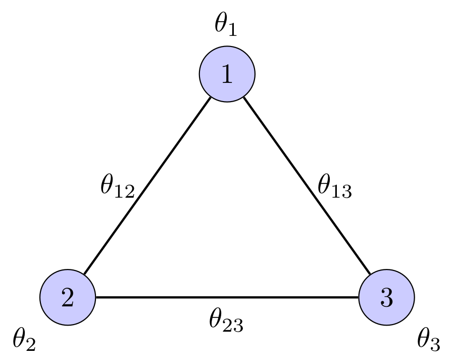

The constraints are more conveniently stated using the so-called minimal representation of binary graphical models [WJ08, Sect. 3.2], that involves the variables11 1 We reuse the symbol for simplicity and only ‘overload’ in this subsection the symbols for local vectors (2.15) by the variables on the left-hand sides of (7.3)
| (7.3) |
and encodes the local vectors (2.15) by
| (7.4) |
Thus, it suffices to use a single variable for every node instead of two variables , and also a single variable for every edge instead of four variables . The local polytope constraints (2.15) then take the form
| (7.5) |
The marginal polytope constraints additionally involve the so-called triangle inequalities [DL97]
| (7.6a) | |||
| (7.6b) | |||
Figure 7.4, right panel, lists the vertices of and the additional vertices of that arise when dropping the subset of constraints (7.6).
We evaluated models generated by randomly sampling the model parameters (2.11): With denoting the uniform distribution on the interval , we set
| (7.7) |
Note the different scale, , , which results in a larger influence of the pairwise terms and hence make inference more difficult. Suppose, for example, that the diagonal terms of are large, which favours the assignment of different labels to the nodes . Then assigning say labels and to the vertices and , respectively, will inherently lead to a large energy contribution due to the assignment to node , no matter if this third label is or , because it must agree with the assignment either to node or to .
Every binary vertex listed by Fig. 7.4, right panel, is the global optimum of both the linear relaxation (1.3) and the original objective function (1.2) in approximately of the scenarios, whereas every non-binary vertex is optimal in approximately .
An example where a non-binary vertex is optimal for the linear relaxation (1.3) is given by the model parameter values
| (7.8) | ||||||
The corresponding solutions of the marginal polytope , the local polytope and our method are listed as Table 1. Due to the non-binary solution returned by the LP-relaxation, rounding in a post-processing step amounts to random guessing. In contrast, our method is able to determine the optimal solution because rounding is smoothly integrated into the overall optimization process.
| Iterations | |||||
| Marginal Polytope | - | ||||
| Local Polytope | - | ||||
| Our Method | |||||
| () | |||||

|

|

|

|
Fig. 7.5 presents the results of the experiments for the minimal cyclic graphical model . In order to assess clearly the influence of the rounding parameter and the smoothing parameter , we evaluated all models for each pair of , where and . These statistics show that our algorithm converges to integral solutions, except for very unbalanced parameter values: strong smoothing with large , weak rounding with small . Within the remaining broad parameter regime, parameter enables to control the influence of rounding. In particular, in agreement with Fig. 7.1 (bottom), less agressive rounding computed labelings closer to the global optimum.
Fig. 7.6 display exactly the same results as Fig. 7.5, except for additional data boxes for three different configurations of parameter values. For instance, using and , our algorithm found in of the experiments an energy with relative error smaller then with respect to the optimal energy. In addition, the algorithm required on average 45 iterations to converge. Using instead and , that is more aggressive rounding in each iteration step (5.4), the average number of iterations reduced to 9, but the accuracy also dropped down to .
Overall, these experiments clearly demonstrate
- •
the ability to control the trade-off between high-quality (low energy) labelings and computational costs in terms of , for all values of below a reasonably large upper bound;
- •
a small or very small number of iterations required to converge, depending on the choice of .
7.3. Comparison to Other Methods
We compared our geometric approach to sequential tree-reweighted message passing (TRWS) [Kol06] and loopy belief propagation [Wei01] (Loopy-BP) based on the OpenGM package [ABK12].

|

|
| Original data | Noisy data |
For this comparison, we evaluated the performance of the methods for a noisy binary labeling scenario depicted by Fig. 7.7. Let denote the noisy image data given on the grid graph with a -neighborhood and as prototypes (labels). The following data term and Potts prior were used,
| (7.9) |
The threshold was used for the normalized average entropy termination criterion (6.12). Figure 7.8 shows the visual reconstruction as well as the corresponding discrete energy values and percentage of correct labels for all three methods. Our method has similar accuracy and returns a slightly better optimal discrete energy level than TRWS and Loopy-BP.

|

|

|
| Geometric | TRWS | Loopy-BP |
| 4977.24 / 98.31% | 4979.61 / 98.07% | 4977.75 / 98.38% |
We investigated again the influence of the rounding mechanism by repeating the same experiment, but using different values of the rounding parameter . As shown by Fig. 7.9, the results confirm the finding of the experiments of the preceding section: More aggressive rounding scheme ( large) leads to faster convergence but yields less regularized results with higher energy values.
|
|

|

|

|
| 4977.24 / 98.31% | 5071.25 / 98.46% | 5472.71 / 96.97% | 7880.64 / 91.25% |
7.4. Non-Uniform (Non-Potts) Priors
We examined the behavior of our approach for a non-Potts prior by applying it to a non-binary labeling problem with noisy input data, as depicted by Fig. 7.10. Our objective is to demonstrate that pre-specified pairwise model parameters (regularization) by a graphical model are properly taken into account.
The label indices corresponding to the five RGB-colors of the original image (Fig. 7.10 right) are
| (7.10) |
Let denote the noisy input image (Fig. 7.10, center panel) given on the grid graph with a -neighborhood. This image was created by randomly selecting of the original image pixels and then uniformly sampling a label at each chosen position. The unary term was defined using the distance and a scaling factor by
| (7.11) |
Now assume additional information about a labeling problem were available. For example, let the RGB-color dark blue in the image represent the direction ”top”, light blue ”bottom”, yellow ”right”, orange ”left” and cyan ”center” (Fig. 7.10 left). Suppose it is known beforehand that ”top” and ”bottom” as well as ”left” and ”right” cannot be adjacent to each other but are separated by another label corresponding to the center. This prior knowledge about the labeling problem was taken into account by specifying non-uniform pairwise model parameters that penalize these unlikely label transitions by a factor of 10:

|

|
|
| original image | noisy image | labels |
| (7.12) |
In words, every entry of corresponding to a label transition (”top”) next to (”bottom”) or (”left”) next to (”right”) has the large penalty value , whereas all other ”natural” configurations are treated as with the Potts prior and smaller penalty value of and , respectively. We point out that no color vectors or any other embedding was used to facilitate this regularization task or to represent it in a more application-specific way. Rather, the non-uniform prior (7.12) was considered as given in terms of some discrete graphical models and its energy function (1.2). On the other hand, the pairs of labels and forming unlikely label transitions can be easily confused by the data term, due to the small distance of the color (feature) vectors representing these labels.
To demonstrate how these non-uniform model parameters influence label assignments, we compared the evaluation of this model against a model with a uniform Potts prior
| (7.13) |
In our experiments, we used the scaling factor for the unaries, step-size , rounding parameter , smoothing parameter and as threshold for the normalized average entropy termination criterion (6.12).

|

|
| Potts | non-Potts |
| Acc : 87.12% | Acc : 99.34% |
The results depicted in Fig. 7.11 clearly show the positive influence of the non-Potts prior (labeling accuracy ) whereas using the Potts prior lowers the accuracy to . This is due to the fact that the color labels and as well as and have a relatively small distance and are therefore not easy to distinguish using both the data term and a Potts prior. On the other hand, the additional prior information about valid label configurations encoded by (7.12) was sufficient to overcome this difficulty, despite using the same data term, and to separate the regions correctly.
8. Conclusion
We presented a novel approach to the evaluation of discrete graphical models in a smooth geometric setting. The novel inference algorithm propagates in parallel ‘Wasserstein messages’ along edges. These messages are lifted to the assignment manifold and drive a Riemannian gradient flow, that terminates at an integral labeling. Local marginalization constraints are satisfied throughout the process. A single parameter enables to trade-off accuracy of optimization and speed of convergence.
Our work motivates to address applications using graphical models with higher edge connectivity, where established inference algorithms based on convex programming noticeably slow down. Likewise, generalizing our approach to tighter relaxations based on hypergraphs and corresponding entropy approximations [YFW05, PA05] seems worth additional investigation. Our future work will leverage the inherent smoothness of our mathematical setting for designing more advanced numerical schemes based on higher-order geometric integration and using multiple spatial scales.
Appendix A Proofs
A.1. Proof of Proposition 4.2
Let be a smooth curve, with , and . We then have
| (A.1) |
where denotes the -th row of the matrix . Since
| (A.2) |
the r.h.s. of (A.1) becomes
| (A.3) |
where we deliberately separated the outer sum into two parts. Let be the function with value if and if . Then the second sum of the expression above reads
| (A.4a) | ||||
| (A.4b) | ||||
| (A.4c) | ||||
| (A.4d) | ||||
where the last equation follows by renaming the indices of summation. Substitution into (A.3) gives
| (A.5a) | ||||
| (A.5b) | ||||
which proves (4.13).
A.2. Proof of Lemma 4.8
We first show that, if is an optimal dual solution, then
| (A.6) |
Let be another optimal dual solution, that is . By (4.21), this equation reads
| (A.7) |
Moreover, due to the optimality conditions (4.27), satisfies
| (A.8) |
with a corresponding primal optimal solution . Hence
| (A.9) |
Using the shorthands
| (A.10) |
we have
| (A.11) |
and therefore
| (A.12) |
Since is strictly convex, this equality can only hold if
| (A.13) |
This shows that and can only differ by a nullspace vector, i.e. we have shown relation (A.6). It remains to show the reverse inclusion, that is vectors characterized by the right-hand side of (4.33) maximize the dual objective function .
Let again be an optimal dual solution, and let be an arbitrary vector. Lemma 4.7 implies that takes the form
| (A.14) |
Now suppose . Then, since , we have
| (A.15a) | ||||
| (A.15b) | ||||
that is .
Acknowledgements
We thank Jan Kuske for sharing with us his framework for running series of experiments efficiently.
References
- [ABK12] B. Andres, T. Beier, and J.H. Kappes, OpenGM: A C++ Library for Discrete Graphical Models, CoRR abs/1206.0111 (2012).
- [AFH+04] A. Aaron, J. Fakcharoenphol, C. Harrelson, R. Krauthgamer, K. Talwar, and E. Tardos, Approximate Classification via Earthmover Metrics, Proc. SODA, 2004, pp. 1079–1087.
- [ÅHS+17] F. Åström, R. Hühnerbein, F. Savarino, J. Recknagel, and C. Schnörr, MAP Image Labeling Using Wasserstein Messages and Geometric Assignment, Proc. SSVM, LCNS 10302, Springer, 2017.
- [Amb89] L. Ambrosio, Variational Problems in SBV and Image Segmentation, Acta Applicandae Mathematica 17 (1989), no. 1, 1–40.
- [ÅPSS17] F. Åström, S. Petra, B. Schmitzer, and C. Schnörr, Image Labeling by Assignment, J. Math. Imag. Vision 58 (2017), no. 2, 211–238.
- [BB97] H. H. Bauschke and J. M. Borwein, Legendre Functions and the Method of Random Bregman Projections, J. Convex Analysis 4 (1997), no. 1, 27–67.
- [BF12] A. Bertozzi and A. Flenner, Diffuse Interface Models on Graphs for Classification of High Dimensional Data, Multiscale Modeling & Simulation 10 (2012), no. 3, 1090–1118.
- [BFPS17] R. Bergmann, J.H. Fitschen, J. Persch, and G. Steidl, Iterative Multiplicative Filters for Data Labeling, Int. J. Computer Vision 123 (2017), no. 3, 435–453.
- [BK04] Y. Boykov and V. Kolmogorov, An Experimental Comparison of Min-Cut/Max-Flow Algorithms for Energy Minimization in Vision, IEEE Trans. Patt. Anal. Mach. !ntell. 26 (2004), no. 9, 1124–1137.
- [Bru06] R.A. Brualdi, Combinatorial Matrix Classes, Cambridge Univ. Press, 2006.
- [BT17] R. Bergmann and D. Tenbrinck, A Graph-Framework for Manifold-Valued Data, CoRR abs/1702.05293 (2017).
- [BV09] S. Boyd and L. Vandenberghe, Convex Optimization, 7th ed., Cambridge Univ. Press, 2009.
- [BVZ01] Y. Boykov, O. Veksler, and R. Zabih, Fast Approximate Energy Minimization via Graph Cuts, IEEE Trans. Patt. Anal. Mach. Intell. 23 (2001), no. 11, 1222–1239.
- [CKNZ05] C. Chekuri, S. Khanna, J. Naor, and L. Zosin, Linear Programming Formulation and Approximation Algorithms for the Metric Labeling Problem, SIAM J. Discr. Math. 18 (2005), no. 3, 608–625.
- [CP16] M. Cuturi and G. Peyré, A Smoothed Dual Approach for Variational Wasserstein Problems, SIAM J. Imag. Sci. 9 (2016), no. 1, 320–343.
- [Cut13] M. Cuturi, Sinkhorn Distances: Lightspeed Computation of Optimal Transport, Advances in Neural Information Processing Systems 26 (C. J. C. Burges, L. Bottou, M. Welling, Z. Ghahramani, and K. Q. Weinberger, eds.), Curran Associates, Inc., 2013, pp. 2292–2300.
- [CZ92] Y. Censor and S.A. Zenios, Proximal Minimization Algorithm with -Functions, J. Optim. Theory Appl. 73 (1992), no. 3, 451–464.
- [Dan66] J.M. Danskin, The Theory of Max-Min, with Applications, SIAM J. Appl. Math. (1966).
- [DL97] M.M. Deza and M. Laurent, Geometry of Cuts and Metrics, Springer, 1997.
- [ELB08] A. Elmoataz, O. Lezoray, and S. Bougleux, Nonlocal Discrete Regularization on Weighted Graphs: A Framework for Image and Manifold Processing, IEEE Trans. Image Proc. 17 (2008), no. 7, 1047–1059.
- [GO08] G. Gilboa and S. Osher, Nonlocal Operators with Applications to Image Processing, Multiscale Model. Simul. 7 (2008), no. 3, 1005–1028.
- [HS10] T. Hazan and A. Shashua, Norm-Product Belief Propagation: Primal-Dual Message-Passing for Approximate Inference, IEEE Trans. Inf. Theory 56 (2010), no. 12, 6294–6316.
- [KAH+15] J.H. Kappes, B. Andres, F.A. Hamprecht, C. Schnörr, S. Nowozin, D. Batra, S. Kim, B.X. Kausler, T. Kröger, J. Lellmann, N. Komodakis, B. Savchynskyy, and C. Rother, A Comparative Study of Modern Inference Techniques for Structured Discrete Energy Minimization Problems, Int. J. Comp. Vision 115 (2015), no. 2, 155–184.
- [Kni08] P.A. Knight, The Sinkhorn-Knopp Algorithm: Convergence and Applications, SIAM J. Matrix Anal. Appl. 30 (2008), no. 1, 261–275.
- [Kol06] V. Kolmogorov, Convergent Tree-Reweighted Message Passing for Energy Minimization, IEEE Trans. Patt. Anal. Mach. Intell. 28 (2006), no. 10, 1568–1583.
- [KPT+17] S. Kolouri, S. Park, M. Thorpe, D. Slepcev, and G.K. Rohde, Optimal mass transport: Signal processing and machine- learning applications, IEEE Signal Proc.�Mag. 34 (2017), no. 4, 43–59, preprint: https://arxiv.org/abs/1609.04767.
- [KT02] J. Kleinberg and E. Tardos, Approximation Algorithms for Classification Problems with Pairwise Relationships: Metric Labeling and Markov Random Fields, Journal of the ACM 49 (2002), no. 5, 616–639.
- [KZ04] V. Kolmogorov and R. Zabih, What Energy Functions Can Be Minimized via Graph Cuts?, IEEE Trans. Patt. Analysis Mach. Intell. 26 (2004), no. 2, 147–159.
- [NN87] Y. Nesterov and A. Nemirovskii, Interior Point Polynomial Algorithms in Convex Programming, Studies in Applied Mathematics, Society for Industrial and Applied Mathematics, 1987.
- [NY83] A.S. Nemirovsky and D.B. Yudin, Problem Complexity and Method Efficiency in Optimization, John Wiley & Sons, 1983.
- [PA05] P. Pakzad and V. Anantharam, Estimation and Marginalization using Kikuchi Approximation Methods, Neural Computation 17 (2005), no. 8, 1836–1873.
- [Pad89] M. Padberg, The Boolean Quadratic Polytope: Some Characteristics, Facets and Relatives, Math. Progr. 45 (1989), 139–172.
- [PDHA97] T. Pham Dinh and L. Hoai An, Convex Analysis Approach to D.C. Programming: Theory, Algorithms and Applications, Acta Math. Vietnamica 22 (1997), no. 1, 289–355.
- [PDHA98] T. Pham Dinh and L.T. Hoai An, A D.C. Optimization Algorithm for Solving the Trust-Region Subproblem, SIAM J. Optimization 8 (1998), no. 2, 476–505.
- [Pey15] G. Peyré, Entropic Approximation of Wasserstein Gradient Flows, SIAM J. Imag. Sci. 8 (2015), no. 4, 2323–2351.
- [RAW10] P. Ravikumar, A. Agarwal, and M. J. Wainwright, Message-Passing for Graph-Structured Linear Programs: Proximal Methods and Rounding Schemes, J. Mach. Learning Res. 11 (2010), 1043–1080.
- [Ren95] J. Renegar, Linear Programming, Complexity Theory and Elementary Functional Analysis, Math. Progr. 70 (1995), 279–351.
- [Roc76] R. T. Rockafellar, Monotone Operators and the Proximal Point Algorithm, SIAM J. Control Optim. 14 (1976), no. 5, 877–898.
- [Roc91] R.T. Rockafellar, On a Special Class of Functions, J. Opt. Theory Appl. 70 (1991), no. 3, 619–621.
- [RW09] R.T. Rockafellar and R. J.-B. Wets, Variational Analysis, 2nd ed., Springer, 2009.
- [Sch90] M.H. Schneider, Matrix Scaling, Entropy Minimization, and Conjugate Duality (II): The Dual Problem, Math. Progr. 48 (1990), 103–124.
- [Sch16a] B. Schmitzer, A Sparse Multiscale Algorithm for Dense Optimal Transport, J. Math. Imag. Vision 56 (2016), no. 2, 238–259.
- [Sch16b] by same author, Stabilized Sparse Scaling Algorithms for Entropy Regularized Transport Problems, CoRR abs/1610.06519 (2016).
- [SHÅ+17] F. Savarino, R. Hühnerbein, F. Åström, J. Recknagel, and C. Schnörr, Numerical Integration of Riemannian Gradient Flows for Image Labeling, Proc. SSVM, LNCS, vol. 10302, Springer, 2017.
- [Sin64] R. Sinkhorn, A Relationship Between Arbitrary Positive Matrices and Doubly Stochastic Matrices, Ann. Math. Statist. 35 (1964), no. 2, 876–879.
- [SSK+16] P. Swoboda, A. Shekhovtsov, J.H. Kappes, C. Schnörr, and B. Savchynskyy, Partial Optimality by Pruning for MAP-Inference with General Graphical Models, IEEE Trans. Patt. Anal. Mach. Intell. 38 (2016), no. 7, 1370–1382.
- [Ter96] T. Terlaky (ed.), Interior Point Methods of Mathematical Programming, Kluwer Acad. Publ., 1996.
- [Wei01] Y. Weiss, Comparing the Mean Field Method and Belief Propagation for Approximate Inference in MRFs, Advanced Mean Field Methods: Theory and Practice, MIT Press, 2001, pp. 229–240.
- [Wer07] T. Werner, A Linear Programming Approach to Max-sum Problem: A Review, IEEE Trans. Patt. Anal. Mach. Intell. 29 (2007), no. 7, 1165–1179.
- [WJ08] M.J. Wainwright and M.I. Jordan, Graphical Models, Exponential Families, and Variational Inference, Found. Trends Mach. Learning 1 (2008), no. 1-2, 1–305.
- [WJW05] M.J. Wainwright, T.S. Jaakola, and A.S. Willsky, MAP Estimation via Agreement on Trees: Message-Passing and Linear Programming, IEEE Trans. Inform. Theory 51 (2005), no. 11, 3697– 3717.
- [YFW05] J.S. Yedidia, W.T. Freeman, and Y. Weiss, Constructing Free-Energy Approximations and Generalized Belief Propagation Algorithms, IEEE Trans. Information Theory 51 (2005), no. 7, 2282–2312.
- [YMW06] C. Yanover, T. Meltzer, and Y. Weiss, Linear Programming Relaxations and Belief Propagation - An Empirical Study, J. Mach. Learning Res. 7 (2006), 1887–1907.