跳到论文正文
W Papers独立论文阅读器 arXiv:1710.01335 论文正文 计算阅读时间 · 0%
引用这篇论文根据当前论文元数据生成,正式投稿前建议核对。


License: arXiv.org perpetual non-exclusive license
arXiv:1710.01335v2 [hep-ph] 05 Mar 2019

Lepton mass effects and angular observables in Λb→Λ(→pπ)ℓ+ℓ−\Lambda_{b}\to\Lambda(\to p\pi)\ell^{+}\ell^{-}

Shibasis Roy Email: shibasisr@imsc.res.in Affiliation: The Institute of Mathematical Sciences, Taramani, Chennai 600113, India
and
Homi Bhabha National Institute Training School Complex,
Anushakti Nagar, Mumbai 400085, India
   Ria Sain Email: riasain@imsc.res.in Affiliation: The Institute of Mathematical Sciences, Taramani, Chennai 600113, India
and
Homi Bhabha National Institute Training School Complex,
Anushakti Nagar, Mumbai 400085, India
   Rahul Sinha Email: sinha@imsc.res.in Affiliation: The Institute of Mathematical Sciences, Taramani, Chennai 600113, India
and
Homi Bhabha National Institute Training School Complex,
Anushakti Nagar, Mumbai 400085, India
August 24, 2026
Abstract

The flavor changing rare decay B→K∗(→Kπ)ℓ+ℓ−B\to{K^{\!*}}(\to K\pi)\ell^{+}\ell^{-} is one of the most studied modes due to its sensitivity to physics beyond the standard model and several discrepancies have come to light among the plethora of observables that are measured. In this paper we revisit the analogous baryonic decay mode Λb→Λ(→pπ)ℓ+ℓ−\Lambda_{b}\rightarrow\Lambda(\to p\pi)\ell^{+}\ell^{-} and we present a complete set of ten angular observables that can be measured using this decay mode. Our calculations are done retaining the finite lepton mass so that the signal of lepton non-universality observed in B→K∗​ℓ+​ℓ−B\to{K^{\!*}}\ell^{+}\ell^{-} can be corroborated by the corresponding baryonic decay mode. We show that due to the parity violating nature of the subsequent Λ→p​π\Lambda\to p\pi decay there exists at least one angular asymmetry that is non-vanishing in the large recoil limit unlike the case in B→K∗​ℓ+​ℓ−B\to{K^{\!*}}\ell^{+}\ell^{-} decay mode, making it particularly sensitive to new physics that violates lepton flavor universality.

I Introduction

It is well known that the rare decay B→K∗​ℓ+​ℓ−B\to{K^{\!*}}\ell^{+}\ell^{-} involves a b→sb\to s flavor changing loop induced transition at the quark level making it sensitive to physics beyond the standard model (SM) [1, 2, 3, 4, 5, 6, 7, 8, 9, 10, 12, 13, 14, 11]. The nature of this decay provides one with a significant number of observables, many of which have been recently measured [15, 16] to a great deal of accuracy. There are several discrepancies observed when compared to the SM predictions, among these, RK(∗)R_{K^{\!(\!*\!)}}, the ratio of the differential decay rate d⁡(B→K(∗)​ℓ+​ℓ−)/d​q2d(B\rightarrow{K^{\!(\!*\!)}}\ell^{+}\ell^{-})/dq^{2}, for ℓ=μ\ell=\mu and ee, has generated a great deal of interest. The deviation of RK(∗)R_{K^{\!(\!*\!)}} from the expected value in the SM imply a challenge to the idea of lepton universality [17] within the SM and points towards a possible evidence of new physics (NP). Naturally the question arises whether we can observe a similar deviation in other decay modes that capture this non-universal behavior of the leptons. This will go a long way in establishing lepton non-universality on firm footing. Here we reexamine the analogous baryonic decay of Λb\Lambda_{b} to Λ\Lambda and a lepton-antilepton pair, where the Λ\Lambda-baryon further decays to proton p+p^{+} and a pion π−\pi^{-} as already discussed by various authors Ref. [18, 19, 20, 21, 22, 23, 24, 25, 26, 27, 28, 29, 30, 31, 32, 33, 34, 35, 36, 39, 37, 38, 40, 41, 42, 43, 44, 45, 46]. The underlying quark level b→s​ℓ+​ℓ−b\rightarrow s\ell^{+}\ell^{-} transition for Λb→Λ​ℓ+​ℓ−\Lambda_{b}\rightarrow\Lambda\ell^{+}\ell^{-} decay is the same as in the well studied B→K(∗)​ℓ+​ℓ−B\rightarrow K^{(*)}\ell^{+}\ell^{-} decay, making it an ideal candidate to study in depth.

Before we study the consequences of lepton non-universality in baryonic decay Λb→Λ(→pπ)ℓ+ℓ−\Lambda_{b}\rightarrow\Lambda(\to p\pi)\ell^{+}\ell^{-}, we recall, that RK(∗)R_{K^{\!(\!*\!)}} is defined [47] within a given range of the dilepton mass squared qmin2q^{2}_{\rm min} to qmax2q^{2}_{\rm max} as,

RK(∗)=∫qmin2qmax2d​Γ​(B→K(∗)​μ+​μ−)d​q2​d​q2∫qmin2qmax2d​Γ​(B→K(∗)​e+​e−)d​q2​d​q2R_{K^{\!(\!*\!)}}=\frac{\displaystyle\int_{q^{2}_{\rm min}}^{q^{2}_{\rm max}}\frac{d\Gamma(B\rightarrow{K^{\!(\!*\!)}}\mu^{+}\mu^{-})}{dq^{2}}dq^{2}}{\displaystyle\int_{q^{2}_{\rm min}}^{q^{2}_{\rm max}}\frac{d\Gamma(B\rightarrow{K^{\!(\!*\!)}}e^{+}e^{-})}{dq^{2}}dq^{2}} (1)

The measured RKR_{K} and RK∗R_{K^{\!*}}, lie systematically below the SM expectations [48, 49]:

RK(q2∈[1:6]GeV2)=0.745−0.074+0.090±0.036,\displaystyle{R_{K}}{(q^{2}\in[1:6]\,\mathrm{Ge\kern-1.00006ptV}^{2})}=\displaystyle 0.745^{+0.090}_{-0.074}\pm 0.036,
RK∗(q2∈[0.045:1.1]GeV2)=0.660−0.070+0.110±0.024,\displaystyle R_{K^{\!*}}(q^{2}\in[0.045:1.1]\,\mathrm{Ge\kern-1.00006ptV}^{2})=\displaystyle{0.660}^{+0.110}_{-0.070}\pm 0.024,
RK∗(q2∈[1.1:6]GeV2)=0.685−0.069+0.113±0.047.\displaystyle R_{K^{\!*}}(q^{2}\in[1.1:6]\,\mathrm{Ge\kern-1.00006ptV}^{2})=\displaystyle 0.685^{+0.113}_{-0.069}\pm 0.047.

In the SM both RKR_{K} and RK∗R_{K^{\!*}} are predicted to be virtually indistinguishable from unity [50] for (q2∈[1:6]GeV2)(q^{2}\in[1:6]\,\mathrm{Ge\kern-1.00006ptV}^{2}), whereas RK∗∼0.9R_{K^{\!*}}\sim 0.9 for q2∈[0.045:1.1]GeV2q^{2}\in[0.045:1.1]\,\mathrm{Ge\kern-1.00006ptV}^{2} owing to a finite mμm_{\mu}. The measurements correspond to a 2.6​σ2.6\sigma, 2.1​σ2.1\sigma and 2.4​σ2.4\sigma shortfalls from the SM expectations respectively.

It is obvious that an observable RΛR_{\Lambda} can be proposed in the same spirit as RK(∗)R_{K^{\!(\!*\!)}} for the corresponding baryonic decay Λb→Λ​ℓ+​ℓ−\Lambda_{b}\to\Lambda\ell^{+}\ell^{-} as,

RΛ=∫qmin2qmax2d​Γ​(Λb→Λ​μ+​μ−)d​q2​d​q2∫qmin2qmax2d​Γ​(Λb→Λ​e+​e−)d​q2​d​q2R_{\Lambda}=\frac{\displaystyle\int_{q^{2}_{\rm min}}^{q^{2}_{\rm max}}\frac{d\Gamma(\Lambda_{b}\rightarrow\Lambda\mu^{+}\mu^{-})}{dq^{2}}dq^{2}}{\displaystyle\int_{q^{2}_{\rm min}}^{q^{2}_{\rm max}}\frac{d\Gamma(\Lambda_{b}\rightarrow\Lambda e^{+}e^{-})}{dq^{2}}dq^{2}} (2)

One should expect the lepton mass effect to play a significant role on RΛR_{\Lambda} in the low-q2q^{2} region, just as in the case of RK(∗)R_{K^{\!(\!*\!)}}. The discrepancy between the SM expectation and the experimentally observed value of RK(∗)R_{K^{\!(\!*\!)}} was largest in the low-q2q^{2} region. The observation of a similar discrepancy in RΛR_{\Lambda} is therefore necessary to substantiate the idea of lepton non-universality in FCNC processes since such an observation cannot be restricted to the celebrated B→K(∗)​ℓ+​ℓ−B\rightarrow K^{(*)}\ell^{+}\ell^{-} alone. In order to disentangle the new physics contribution that may manifest as lepton non-universality, one must take into account the SM contribution to RΛR_{\Lambda} including the effect of finite leptons mass [51, 52]. We therefore derive the expression for RΛR_{\Lambda} without any approximation.

Another salient feature of the Λb→Λ(→p+π−)ℓ+ℓ−\Lambda_{b}\rightarrow\Lambda(\rightarrow p^{+}\pi^{-})\ell^{+}\ell^{-} decay, is the wealth of information carried by the angular observables expressed in terms of the angular asymmetries, of which the forward-backward asymmetry in the hadron angle θΛ\theta_{\Lambda} is of particular interest. We show that due to the parity violating nature of the Λ→p​π\Lambda\to p\pi decay angular asymmetry are non-vanishing in the large recoil or low-q2q^{2} limit unlike the case in B→K∗(→Kπ)ℓ+ℓ−B\to{K^{\!*}}(\to K\pi)\ell^{+}\ell^{-}, making it particularly sensitive to new physics that violates lepton flavor universality. This follows since ratios of hadronic forward-backward asymmetry for ℓ=μ\ell=\mu and ℓ=e\ell=e, in the low-q2q^{2} region, is a ratio of two finite quantities for Λb→Λ(→p+π−)ℓ+ℓ−\Lambda_{b}\rightarrow\Lambda(\rightarrow p^{+}\pi^{-})\ell^{+}\ell^{-} decay. It may be recollected that all asymmetries for B→K∗​ℓ+​ℓ−B\to{K^{\!*}}\ell^{+}\ell^{-} decay mode vanish in the low-q2q^{2} region [11].

Our paper is arranged in the following way; in Sec. II we derive the complete angular distribution consisting ten angular observables retaining all the helicities and lepton mass. Sec. III is devoted to the calculation of hadronic helicity amplitudes in terms of known parameters namely the Wilson coefficients and form factors. In Sec. IV the decay rate and angular asymmetries are written in terms of the helicity amplitudes. We also define observables that are free from hadronic uncertainties. Finally we conclude how these observables can play an important role in pinning down lepton-universality violating new physics.

II The decay of Λb→Λ(→p+π−)ℓ+ℓ−\Lambda_{b}\rightarrow\Lambda(\rightarrow p^{+}\pi^{-})\ell^{+}\ell^{-}

The process Λb→Λ(→pπ−)+jeff(→ℓ+ℓ−)\Lambda_{b}\rightarrow\Lambda(\rightarrow p\pi^{-})+j_{\text{eff}}(\rightarrow\ell^{+}\ell^{-}) can be thought of as a sequential decay where it is assumed that the daughter Λ\Lambda-baryon is onshell and subsequently decays resonantly. This enables one to write down a joint angular decay distribution  [53, 54, 55, 56] which is described fully by four independent kinematic variables: the dilepton invariant mass squared q2q^{2}, the polar angles θl\theta_{l}, θΛ\theta_{\Lambda} and the azimuthal angle ϕ\phi defined by the decay products in their respective centre-of-mass (CM) frames. At this point we would like to clarify that in our convention we have chosen θl\theta_{l} to be the angle between the lepton (ℓ−\ell^{-}) and the flight direction of the jeffj_{\text{eff}}-system, θΛ\theta_{\Lambda} to be the angle between the nucleon (pp) and the Λ\Lambda flight direction and ϕ\phi to be the angle between the two decay planes. The angular distribution involves the helicity amplitudes HλΛ,λj​(J)H_{\lambda_{\Lambda},\lambda_{j}}(J) for the decay Λb→Λ+jeff\Lambda_{b}\rightarrow\Lambda+j_{\text{eff}}, hλ1,λ2ah^{a}_{\lambda_{1},\lambda_{2}} for the decay jeff→ℓ+​ℓ−j_{\text{eff}}\rightarrow\ell^{+}\ell^{-} and hλp,0h_{\lambda_{p},0} for the decay Λ→p+π−\Lambda\rightarrow p+\pi^{-}. The joint angular distribution for a unpolarized Λb\Lambda_{b} decay is given by,

K⁡(q2,θl,θΛ,ϕ)=\displaystyle K(q^{2},\theta_{l},\theta_{\Lambda},\phi)= ∑J,J′,Mi=±12,Mi′=12,λj,λj′,a,a′,λΛ,λΛ′,λp,λ1,λ2HλΛ,λja(J)HλΛ′,λj′a′∗(J′)ρMi,Mi′\displaystyle\sum_{J,J^{\prime},M_{i}=\pm\frac{1}{2},M_{i}^{\prime}=\frac{1}{2},\lambda_{j},\lambda_{j}^{\prime},a,a^{\prime},\lambda_{\Lambda},\lambda_{\Lambda}^{\prime},\lambda_{p},\lambda_{1},\lambda_{2}}H_{\lambda_{\Lambda},\lambda_{j}}^{a}(J)H_{\lambda_{\Lambda^{\prime}},\lambda_{j}^{\prime}}^{a^{\prime}*}(J^{\prime})\rho_{M_{i},M_{i}^{\prime}} (3)
𝒟Mi,λΛ−λj12(0,0,0)𝒟Mi′,λΛ′−λj′∗12(0,0,0)δJ​J′hλ1,λ2a(J)hλ1,λ2a′∗(J′)\displaystyle\mathcal{D}^{\frac{1}{2}}_{M_{i},\lambda_{\Lambda}-\lambda_{j}}(0,0,0)\mathcal{D}^{*\frac{1}{2}}_{M_{i}^{\prime},\lambda_{\Lambda}^{\prime}-\lambda_{j}^{\prime}}(0,0,0)\delta_{JJ^{\prime}}h^{a}_{\lambda_{1},\lambda_{2}}(J)h^{a^{\prime}*}_{\lambda_{1},\lambda_{2}}(J^{\prime})
𝒟λj,λ1−λ2J​(0,θl,0)​𝒟λj′,λ1−λ2∗J′​(0,θl,0)​hλp,0​hλp,0∗\displaystyle\mathcal{D}^{J}_{\lambda_{j},\lambda_{1}-\lambda_{2}}(0,\theta_{l},0)\mathcal{D}^{*J^{\prime}}_{\lambda_{j}^{\prime},\lambda_{1}-\lambda_{2}}(0,\theta_{l},0)h_{\lambda_{p},0}h_{\lambda_{p},0}^{*}
𝒟λΛ,λp12​(−ϕ,θΛ,ϕ)​𝒟λΛ′,λp∗12​(−ϕ,θΛ,ϕ)\displaystyle\mathcal{D}^{\frac{1}{2}}_{\lambda_{\Lambda},\lambda_{p}}(-\phi,\theta_{\Lambda},\phi)\mathcal{D}^{*\frac{1}{2}}_{\lambda_{\Lambda^{\prime}},\lambda_{p}}(-\phi,\theta_{\Lambda},\phi)

The polarization density matrix of Λb\Lambda_{b}, ρMi,Mi′\rho_{M_{i},M_{i}^{\prime}} in Eqn (3) is a hermitean 2×\times2 matrix, with Tr​(ρ)\text{Tr}(\rho) = 1. ρ+⁣+\rho_{++} and ρ−⁣−\rho_{--} represent the probability that the initial state Λb\Lambda_{b} has Mi=12M_{i}=\frac{1}{2} and Mi=−12M_{i}=-\frac{1}{2} respectively. For an unpolarized sample of Λb\Lambda_{b}-baryon, ρMi,Mi′=12​δMi,Mi′\rho_{M_{i},M_{i}^{\prime}}=\frac{1}{2}\delta_{M_{i},M_{i}^{\prime}}. In the rest frame of Λb\Lambda_{b}-baryon, the daughter Λ\Lambda-baryon and jeffj_{\text{eff}} fly back to back and without loss of generality it can be assumed that the motion of Λ\Lambda and jeffj_{\text{eff}} is along the zz-axis. This reduces the first two Wigner’s D functions to Kronecker delta functions δMi,λΛ−λj\delta_{M_{i},\lambda_{\Lambda}-\lambda_{j}} and δMi′,λΛ′−λj′\delta_{M_{i}^{\prime},\lambda_{\Lambda}^{\prime}-\lambda_{j}^{\prime}} respectively, where Mi,Mi′=±12M_{i},\ M_{i}^{\prime}=\pm\frac{1}{2}. After summing over Mi,Mi′M_{i},\ M_{i}^{\prime} we are left with a Kronecker delta δλΛ′−λj′,λΛ−λj\delta_{\lambda_{\Lambda}^{\prime}-\lambda_{j}^{\prime},\lambda_{\Lambda}-\lambda_{j}} which signifies the fact that we considered the decay of an unpolarized Λb\Lambda_{b}. We also observe that |λΛ′−λj′|=|λΛ−λj|=12|\lambda_{\Lambda}^{\prime}-\lambda_{j}^{\prime}|=|\lambda_{\Lambda}-\lambda_{j}|=\frac{1}{2} as the initial Λb\Lambda_{b} is spin-1/2. This condition further restricts the values λΛ,λj\lambda_{\Lambda},\ \lambda_{j} can take and the fact has been already taken into account while calculating K⁡(q2,θl,θΛ,ϕ)K(q^{2},\theta_{l},\theta_{\Lambda},\phi). The choice of possible values for λΛ\lambda_{\Lambda} and λj\lambda_{j} are depicted in Table 1.

The hadronic helicity amplitudes HλΛ,λja​(J)H_{\lambda_{\Lambda},\lambda_{j}}^{a}(J) contain all the information of the Λb→Λ+jeff\Lambda_{b}\rightarrow\Lambda+j_{\text{eff}} transition in terms of the relevant form factors and Wilson coefficients parametrizing the underlying b→s​ℓ+​ℓ−b\rightarrow s\ell^{+}\ell^{-} process, explained in detail in Sec III. In case of a spin-12\frac{1}{2} Λb\Lambda_{b} baryon decaying to an intermediate onshell spin-12\frac{1}{2} Λ\Lambda baryon there are four hardonic helicitiy amplitudes HλΛ,λja​(J)H_{\lambda_{\Lambda},\lambda_{j}}^{a}(J), where the index ‘aa’ denotes whether the hadronic helicity amplitudes multiply the lepton vector current (a=1a=1), or the axial vector current (a=2a=2). The label (JJ) takes the values (J=0J=0) with λj=t\lambda_{j}=t and (J=1J=1) with λj=±1,0\lambda_{j}=\pm 1,0 for scalar and vector parts of the effctive current jeffj_{\text{eff}} respectively.

λΛ\lambda_{\Lambda} λj\lambda_{j} MiM_{i}
1/21/2 1 −1/2-1/2
1/21/2 0 1/21/2
−1/2-1/2 -1 1/21/2
−1/2-1/2 0 −1/2-1/2
Table 1: The possible values of λΛ\lambda_{\Lambda} and λj\lambda_{j}

Let us also discuss here the helicity amplitudes hλj;λ1,λ2ah^{a}_{\lambda_{j};\lambda_{1},\lambda_{2}} appearing in Eq. (3) describing the process jeff→ℓ+​ℓ−j_{\text{eff}}\rightarrow\ell^{+}\ell^{-}, where λj=λ1−λ2\lambda_{j}=\lambda_{1}-\lambda_{2}. Explicitly,

a=1​(V):hλj;λ1,λ21​(J)=u¯1​(λ1)​γμ​v2​(λ2)​ϵμ​(λj),\displaystyle a=1\text{(V)}:\quad h^{1}_{\lambda_{j};\lambda_{1},\lambda_{2}}(J)=\bar{u}_{1}(\lambda_{1})\gamma_{\mu}v_{2}(\lambda_{2})\epsilon^{\mu}(\lambda_{j}),\quad
(4)
a=2​(A):hλj;λ1,λ22​(J)=u¯1​(λ1)​γμ​γ5​v2​(λ2)​ϵμ​(λj).\displaystyle a=2\text{(A)}:\quad h^{2}_{\lambda_{j};\lambda_{1},\lambda_{2}}(J)=\bar{u}_{1}(\lambda_{1})\gamma_{\mu}\gamma_{5}v_{2}(\lambda_{2})\epsilon^{\mu}(\lambda_{j}).

These helicity amplitudes are evaluated in the (ℓ+​ℓ−\ell^{+}\ell^{-}) CM frame with ℓ−\ell^{-} defined in the −z-z direction. The label (JJ) is the same as defined previously and takes the values (J=0J=0) with λj=0​(t)\lambda_{j}=0(t) and (J=1J=1) with λj=±1,0\lambda_{j}=\pm 1,0 for scalar and vector parts of the effective current jeffj_{\text{eff}} respectively. The leptonic helicity amplitudes are calculated and given below:

ht;12,121​(J=0)\displaystyle h^{1}_{t;\frac{1}{2},\frac{1}{2}}(J=0) =0,\displaystyle=0,
ht;12,122​(J=0)\displaystyle h^{2}_{t;\frac{1}{2},\frac{1}{2}}(J=0) =2​mℓ,\displaystyle=2m_{\ell},
h0;12,121​(J=1)\displaystyle h^{1}_{0;\frac{1}{2},\frac{1}{2}}(J=1) =2​mℓ,\displaystyle=2m_{\ell},
h0;12,122​(J=1)\displaystyle h^{2}_{0;\frac{1}{2},\frac{1}{2}}(J=1) =0,\displaystyle=0,
h1;12,−121​(J=1)\displaystyle h^{1}_{1;\frac{1}{2},-\frac{1}{2}}(J=1) =−2​q2,\displaystyle=-\sqrt{2q^{2}},
h1;12,−122​(J=1)\displaystyle h^{2}_{1;\frac{1}{2},-\frac{1}{2}}(J=1) =2​q2​v,\displaystyle=\sqrt{2q^{2}}v, (5)

where v=1−4​mℓ2/q2v=\sqrt{1-4m_{\ell}^{2}/q^{2}} is the velocity of the lepton in the (ℓ+​ℓ−\ell^{+}\ell^{-}) CM frame, mℓm_{\ell} being the lepton mass.
As the leptonic current is either purely vector or axial-vector in nature, they have definite parity properties which are given by,

h−λj;−λ1,−λ21\displaystyle h^{1}_{-\lambda_{j};-\lambda_{1},-\lambda_{2}} =hλj;λ1,λ21,\displaystyle=h^{1}_{\lambda_{j};\lambda_{1},\lambda_{2}}, (6)
h−λj;−λ1,−λ22\displaystyle h^{2}_{-\lambda_{j};-\lambda_{1},-\lambda_{2}} =−hλj;λ1,λ22.\displaystyle=-h^{2}_{\lambda_{j};\lambda_{1},\lambda_{2}}. (7)

Finally, we move on to the helicity amplitudes hλp,0h_{\lambda_{p},0} describing the decay Λ→p​π−\Lambda\rightarrow p\pi^{-}. We note that this decay is in itself parity non-conserving in addition to the main decay of Λb→Λ+jeff\Lambda_{b}\rightarrow\Lambda+j_{\text{eff}}. This is in contrast to the well-studied mesonic analouge of B→K∗​ℓ+​ℓ−B\rightarrow K^{*}\ell^{+}\ell^{-}, where the K∗K^{*} meson subsequently decays to K​πK\pi conserving parity. Also there is only one helicity amplitude for K∗→K​πK^{*}\rightarrow K\pi compared to two helicity ampltudes as is the case for the Λ→p​π−\Lambda\rightarrow p\pi^{-} decay. The parity non-conserving nature of the Λ→p​π−\Lambda\rightarrow p\pi^{-} decay leads to the forward-backward asymmetry on the hadron side (angular asymmetry in θΛ\theta_{\Lambda}) as well as double asymmetries (angular asymmetry in θΛ\theta_{\Lambda} and θl\theta_{l}), in addition to the lepton side (angular asymmetry in θl\theta_{l} ).

II.1 Full angular distribution

\displaystyle K⁡(q2,θl,θΛ,ϕ)\displaystyle K(q^{2},\theta_{l},\theta_{\Lambda},\phi)\, (8)
=(K1​s​ssin2θℓ+K1​c​ccos2θℓ+K1​ccosθℓ)\displaystyle=\big(K_{1ss}\sin^{2}\theta_{\ell}+\,K_{1cc}\cos^{2}\theta_{\ell}+K_{1c}\cos\theta_{\ell}\big)\,
+(K2​s​ssin2θℓ+K2​c​ccos2θℓ+K2​ccosθℓ)cosθΛ\displaystyle+\big(K_{2ss}\sin^{2}\theta_{\ell}+\,K_{2cc}\cos^{2}\theta_{\ell}+K_{2c}\cos\theta_{\ell}\big)\cos\theta_{\Lambda}
+(K3​s​csinθℓcosθℓ+K3​ssinθℓ)sinθΛsinϕ\displaystyle+\big(K_{3sc}\sin\theta_{\ell}\cos\theta_{\ell}+K_{3s}\sin\theta_{\ell}\big)\sin\theta_{\Lambda}\sin\phi
+(K4​s​csinθℓcosθℓ+K4​ssinθℓ)sinθΛcosϕ.\displaystyle+\big(K_{4sc}\sin\theta_{\ell}\cos\theta_{\ell}+K_{4s}\sin\theta_{\ell}\big)\sin\theta_{\Lambda}\cos\phi\,.

K1​s​s⋯K4​sK_{1ss}\cdots K_{4s} are the angular observables and they are functions of q2q^{2} and mℓm_{\ell} [20, 12]. We cast this angular distribution in terms of orthogonal Legendre functions which is advantageous as the angular observables are uncorrelated to each other. We then provide a set of relations between the K1​s​s⋯K4​sK_{1ss}\cdots K_{4s} and the new uncorrelated angular observables I1⋯I10I_{1}\cdots I_{10} given below,

K1​s​s=I1−I22,K1​c​c=I1+I2,\displaystyle K_{1ss}=I_{1}-\frac{I_{2}}{2},\ K_{1cc}=I_{1}+I_{2},
K2​s​s=I4−I52,K2​c​c=I4+I5,\displaystyle K_{2ss}=I_{4}-\frac{I_{5}}{2},\ K_{2cc}=I_{4}+I_{5}, (9)
K1​c=I3,K2​c=I6,K4​s​c=I7,\displaystyle K_{1c}=I_{3},\ K_{2c}=I_{6},\ K_{4sc}=I_{7},
K4​s=I8,K3​s​c=I9,K3​s=I10.\displaystyle K_{4s}=I_{8},\ K_{3sc}=I_{9},\ K_{3s}=I_{10}.

The expressions for I1⋯I10I_{1}\cdots I_{10} are derived in terms of the transversality amplitudes in Sec. III and are presented in Table 2.

In Eq. (8) full angular analysis is presented from which the complete set of q2q^{2} dependent observables are extracted. Once a good deal of statistics is available in future it is expected that full reconstruction of the angular observables is possible . For the sake of completeness here we also provide angular observables made of partially integrated distributions. Starting from full angular distribution (Eq. (8)) the three uniangular distributions can be obtained:

d2​Γd​q2​d​ϕ=14​(16​I1+π2​I8​cos⁡ϕ+π2​I10​sin⁡ϕ)\frac{d^{2}\Gamma}{dq^{2}d\phi}=\frac{1}{4}(16I_{1}+\pi^{2}I_{8}\cos\phi+\pi^{2}I_{10}\sin\phi) (10)
d2​Γdq2dcosθℓ=−π(4I1+I2(1+3cos2θℓ)+4I3cosθℓ)\frac{d^{2}\Gamma}{dq^{2}\,d\cos\theta_{\ell}}=-\pi(4I_{1}+I_{2}(1+3\cos 2\theta_{\ell})+4I_{3}\cos\theta_{\ell}) (11)
d2​Γdq2dcosθΛ=−4π(I1+I4cosθΛ)\frac{d^{2}\Gamma}{dq^{2}d\cos\theta_{\Lambda}}=-4\pi(I_{1}+I_{4}\cos\theta_{\Lambda}) (12)

III Hadronic helicity amplitudes

In Eq.(8) we have obtained the angular distribution of Λb​(12)→Λ⁡(12)+J⁡(0,1)\Lambda_{b}(\frac{1}{2})\rightarrow\Lambda(\frac{1}{2})+J(0,1), where the Λ\Lambda further decays to p​π−p\pi^{-}. Before calculating the helicity amplitudes of the primary decay let us go through the details of the subsequent hadronic decay briefly. An onshell spin-12\frac{1}{2} Λ\Lambda-baryon (u​d​suds) goes into an onshell proton pp (u​u​duud) and a pion π−\pi^{-} via a parity non-conserving weak decay that involvles two hadronic couplings aa and bb. The matrix element for this decay can be written in the following way,

⟨p⁡(k1)​π​(k2)|(d¯​γμ​PL​u)​(u¯​γμ​PL​s)|Λ⁡(k)⟩=u¯​(k1)​[(a+b​γ5)]​u​(k).\langle p(k_{1})\pi(k_{2})|(\bar{d}\gamma^{\mu}P_{L}u)(\bar{u}\gamma_{\mu}P_{L}s)|\Lambda(k)\rangle\\ =\bar{u}(k_{1})\Big[\big(a+b\gamma^{5}\big)\Big]u(k). (13)

We also note that the helicity amplitudes hλp,0h_{\lambda_{p},0} defined in Eq. (3) describe the same decay Λ→p+​π−\Lambda\rightarrow p^{+}\pi^{-}. Moreover it is clear that there are only two helicity amplitudes as λp\lambda_{p} takes values ±12\pm\frac{1}{2}. From a separate measurement of the Λ→p+​π−\Lambda\rightarrow p^{+}\pi^{-} decay width and the polarization asymmetry these two helicity amplitudes can be inferred which is equivalent to the extraction of the two hadronic couplings aa and bb.

To calculate the hadronic helicity amplitudes of the primary decay which in turn can be related to the invariant form factors, we start with the Hamiltonian for the decay described in Ref [57] .

The matrix element for the decay Λb→Λ​ℓ¯​ℓ\Lambda_{b}\to\Lambda\bar{\ell}\ell is defined by,

ℳ⁡(Λb→CLOSE\displaystyle\mathcal{M}(\Lambda_{b}\to Λℓ¯ℓ)=GF2α​λt2​π[C9eff⟨Λ|s¯γμ(1−γ5)b|Λb⟩ℓ¯γμℓ\displaystyle\Lambda\bar{\ell}\ell)=\frac{G_{F}}{\sqrt{2}}\frac{\alpha\lambda_{t}}{2\,\pi}[C_{9}^{\rm eff}\,\langle\Lambda\,|\,\bar{s}\,\gamma^{\mu}(1-\gamma^{5})b\,|\,\Lambda_{b}\rangle\,\bar{\ell}\gamma_{\mu}\ell
+C10​⟨Λ|s¯​γμ​(1−γ5)​b|Λb⟩​ℓ¯​γμ​γ5​ℓ\displaystyle+C_{10}\,\langle\Lambda\,|\,\bar{s}\,\gamma^{\mu}(1-\gamma^{5})b\,|\,\Lambda_{b}\rangle\,\bar{\ell}\gamma_{\mu}\gamma_{5}\ell (14)
−2​mbq2C7eff⟨Λ|s¯iσμ​q(1+γ5)b|Λb⟩ℓ¯γμℓ]\displaystyle-\frac{2m_{b}}{q^{2}}\,C_{7}^{\rm eff}\,\langle\Lambda\,|\,\bar{s}\,i\sigma^{\mu q}\,(1+\gamma^{5})\,\,b\,|\,\Lambda_{b}\rangle\,\bar{\ell}\gamma_{\mu}\ell]\,

where Ci′C_{i}^{\prime}s are the Wilson coefficients, λt≡Vt​s∗​Vt​b\lambda_{t}\equiv V^{*}_{ts}V_{tb} and mbm_{b} is the bb-quark mass. For this paper all the values of the Wilson coefficients have been been taken from Ref  [19]. The hadronic matrix elements written in terms of dimension less form factors as:

⟨Λ⁡(k)​|s¯​γμ​b|​Λb​(p)⟩\displaystyle\langle\Lambda(k)\,|\,\bar{s}\,\gamma^{\mu}\,b\,|\Lambda_{b}(p)\rangle =\displaystyle= u¯2​(p2)​[f1V​(q2)​γμ−f2V​(q2)​i​σμ​q/mΛb+f3V​(q2)​qμ/mΛb]​u1​(p1),\displaystyle\bar{u}_{2}(p_{2})\Big[f^{V}_{1}(q^{2})\gamma^{\mu}-f^{V}_{2}(q^{2})i\sigma^{\mu q}/m_{\Lambda_{b}}+f^{V}_{3}(q^{2})q^{\mu}/m_{\Lambda_{b}}\Big]u_{1}(p_{1})\,,
⟨Λ⁡(k)​|s¯​γμ​γ5​b|​Λb​(p)⟩\displaystyle\langle\Lambda(k)\,|\,\bar{s}\,\gamma^{\mu}\gamma^{5}\,b\,|\Lambda_{b}(p)\rangle =\displaystyle= u¯2​(p2)​[f1A​(q2)​γμ−f2A​(q2)​i​σμ​q/mΛb+f3A​(q2)​qμ/mΛb]​γ5​u1​(p1),\displaystyle\bar{u}_{2}(p_{2})\Big[f^{A}_{1}(q^{2})\gamma^{\mu}-f^{A}_{2}(q^{2})i\sigma^{\mu q}/m_{\Lambda_{b}}+f^{A}_{3}(q^{2})q^{\mu}/m_{\Lambda_{b}}\Big]\gamma^{5}u_{1}(p_{1})\,,
⟨Λ⁡(k)​|s¯​i​σμ​q/mΛb​b|​Λb​(p)⟩\displaystyle\langle\Lambda(k)\,|\,\bar{s}\,i\sigma^{\mu q}/m_{\Lambda_{b}}\,b\,|\Lambda_{b}(p)\rangle =\displaystyle= u¯2​(p2)​[f1T​V​(q2)​(γμ​q2−qμ​​q)/mΛb2−f2T​V​(q2)​i​σμ​q/mΛb]​u1​(p1),\displaystyle\bar{u}_{2}(p_{2})\Big[f^{TV}_{1}(q^{2})(\gamma^{\mu}q^{2}-q^{\mu}\not\!q)/m_{\Lambda_{b}}^{2}-f^{TV}_{2}(q^{2})i\sigma^{\mu q}/m_{\Lambda_{b}}\Big]u_{1}(p_{1})\,,
⟨Λ⁡(k)​|s¯​i​σμ​q​γ5/mΛb​b|​Λb​(p)⟩\displaystyle\langle\Lambda(k)\,|\,\bar{s}\,i\sigma^{\mu q}\gamma^{5}/m_{\Lambda_{b}}\,b\,|\Lambda_{b}(p)\rangle =\displaystyle= u¯2​(p2)​[f1T​A​(q2)​(γμ​q2−qμ​​q)/mΛb2−f2T​A​(q2)​i​σμ​q/mΛb]​γ5​u1​(p1).\displaystyle\bar{u}_{2}(p_{2})\Big[f^{TA}_{1}(q^{2})(\gamma^{\mu}q^{2}-q^{\mu}\not\!q)/m_{\Lambda_{b}}^{2}-f^{TA}_{2}(q^{2})i\sigma^{\mu q}/m_{\Lambda_{b}}\Big]\gamma^{5}u_{1}(p_{1})\,. (15)

The helicity amplitudes Hλ2,λjaH^{a}_{\lambda_{2},\lambda_{j}}, are expressed by following relation,

HλΛ,λja=Mμa​(λΛ)​ϵ∗μ​(λj).H^{a}_{\lambda_{\Lambda},\lambda_{j}}=M^{a}_{\mu}(\lambda_{\Lambda})\epsilon^{*\mu}(\lambda_{j}). (16)

MμaM^{a}_{\mu} are the hadronic matrix elements defined in Eq. (15). As before, the labels λj\lambda_{j} and λΛ\lambda_{\Lambda} denote the helicities of the effective current and daughter baryon respectively. We shall work in the rest frame of the parent baryon Λb\Lambda_{b} where the daughter baryon Λ\Lambda moving in the positive zz direction and the effective current moving along the negative zz-axis. The relevant momenta that describe the motion of particles in this frame are given below,

pμ=(mΛb,0,0,0),kμ=(E2,0,0,p2),qμ=(q0,0,0,−p2),p^{\mu}=(m_{\Lambda_{b}},0,0,0),\ k^{\mu}=(E_{2},0,0,p_{2}),\ q^{\mu}=(q_{0},0,0,-p_{2}),

where q0=12​mΛb​(mΛb2−mΛ2+q2)q_{0}=\frac{1}{2m_{\Lambda_{b}}}(m_{\Lambda_{b}}^{2}-m_{\Lambda}^{2}+q^{2}) and E2=(mΛb−q0)=(mΛb2+mΛ2−q2)/2​mΛbE_{2}=(m_{\Lambda_{b}}-q_{0})=(m_{\Lambda_{b}}^{2}+m_{\Lambda}^{2}-q^{2})/2m_{\Lambda_{b}}. The helicity of the particles is fixed by angular momentum relation through the equation Mi=λΛ−λjM_{i}=\lambda_{\Lambda}-\lambda_{j}. The J=12J=\frac{1}{2} baryon helicity spinors are given by,

u¯2​(k→=p2​z^,±12)\displaystyle\bar{u}_{2}\Big(\vec{k}=p_{2}\ \hat{z},\pm\frac{1}{2}\Big) =E2+mΛ​(χ±†​∓|p2|E2+mΛ​χ±†),\displaystyle=\sqrt{E_{2}+m_{\Lambda}}\begin{pmatrix}\chi^{\dagger}_{\pm}\frac{\mp|p_{2}|}{E_{2}+m_{\Lambda}}\chi^{\dagger}_{\pm}\end{pmatrix}, (17)
u1​(p→=0,±12)\displaystyle u_{1}\Big(\vec{p}=0,\pm\frac{1}{2}\Big) =2​mΛb​(χ±0),\displaystyle=\sqrt{2m_{\Lambda_{b}}}\begin{pmatrix}\chi_{\pm}\\ 0\end{pmatrix}, (18)

where χ+=(10)\chi_{+}=\begin{pmatrix}1\\ 0\end{pmatrix} and χ−=(01)\chi_{-}=\begin{pmatrix}0\\ 1\end{pmatrix} are two-component Pauli spinors.

The polarization vectors of the effective current JeffJ_{\text{eff}} moving along negative zz-axis look like,

ϵμ​(t)=1q2​(q0,0,0,−p​2),\epsilon^{\mu}(t)=\frac{1}{\sqrt{q^{2}}}(q_{0},0,0,-p2),
ϵμ​(±)=12​(0,±1,−i,0)\epsilon^{\mu}(\pm)=\frac{1}{\sqrt{2}}(0,\pm 1,-i,0) (19)
ϵμ​(0)=1q2​(p2,0,0,−q0).\epsilon^{\mu}(0)=\frac{1}{\sqrt{q^{2}}}(p_{2},0,0,-q_{0}).

They satisfy the qμ​ϵμ=0q_{\mu}\epsilon^{\mu}=0 equation, qμq_{\mu} being the momentum four-vector of the effective current. We also note that hadronic helicity can be expressed as,

HλΛ,λja=HλΛ,λjV​a−HλΛ,λjA​aH^{a}_{\lambda_{\Lambda},\lambda_{j}}=H^{Va}_{\lambda_{\Lambda},\lambda_{j}}-H^{Aa}_{\lambda_{\Lambda},\lambda_{j}} (20)

where, HλΛ,λjV​aH^{Va}_{\lambda_{\Lambda},\lambda_{j}}, HλΛ,λjA​aH^{Aa}_{\lambda_{\Lambda},\lambda_{j}} are the vector and axial-vector part of the helicity amplitudes respectively. HλΛ,λjV​aH^{Va}_{\lambda_{\Lambda},\lambda_{j}}, HλΛ,λjA​aH^{Aa}_{\lambda_{\Lambda},\lambda_{j}} have definite parity properties;

H−λΛ,−λjV​a=HλΛ,λjV​aH−λΛ,−λjA​a=−HλΛ,λjA​a.H^{Va}_{-\lambda_{\Lambda},-\lambda_{j}}=H^{Va}_{\lambda_{\Lambda},\lambda_{j}}\qquad H^{Aa}_{-\lambda_{\Lambda},-\lambda_{j}}=-H^{Aa}_{\lambda_{\Lambda},\lambda_{j}}. (21)

Different hadronic helicity amplitudes that take part in the decay are presented below,

H12​tV​a\displaystyle H^{Va}_{\frac{1}{2}t} =\displaystyle= Q+q2​(M−​F1V​a+q2mΛb​F3V​a),\displaystyle\sqrt{\frac{Q_{+}}{q^{2}}}\,\biggl(M_{-}\,F_{1}^{Va}+\frac{q^{2}}{m_{\Lambda_{b}}}\,F_{3}^{Va}\biggr)\,,
H12​1V​a\displaystyle H^{Va}_{\frac{1}{2}1} =\displaystyle= 2​Q−​(F1V​a+M+mΛb​F2V​a),\displaystyle\sqrt{2Q_{-}}\,\biggl(F_{1}^{Va}+\frac{M_{+}}{m_{\Lambda_{b}}}\,F_{2}^{Va}\biggr)\,,
H12​0V​a\displaystyle H^{Va}_{\frac{1}{2}0} =\displaystyle= Q−q2​(M+​F1V​a+q2mΛb​F2V​a),\displaystyle\sqrt{\frac{Q_{-}}{q^{2}}}\,\biggl(M_{+}\,F_{1}^{Va}+\frac{q^{2}}{m_{\Lambda_{b}}}\,F_{2}^{Va}\biggr)\,, (22)
H12​tA​a\displaystyle H^{Aa}_{\frac{1}{2}t} =\displaystyle= Q−q2​(M+​F1A​a−q2mΛb​F3A​a),\displaystyle\sqrt{\frac{Q_{-}}{q^{2}}}\,\biggl(M_{+}\,F_{1}^{Aa}-\frac{q^{2}}{m_{\Lambda_{b}}}\,F_{3}^{Aa}\biggr)\,,
H12​1A​a\displaystyle H^{Aa}_{\frac{1}{2}1} =\displaystyle= 2​Q+​(F1A​a−M−mΛb​F2A​a),\displaystyle\sqrt{2Q_{+}}\,\biggl(F_{1}^{Aa}-\frac{M_{-}}{m_{\Lambda_{b}}}\,F_{2}^{Aa}\biggr)\,,
H12​0A​a\displaystyle H^{Aa}_{\frac{1}{2}0} =\displaystyle= Q+q2​(M−​F1A​a−q2mΛb​F2A​a),\displaystyle\sqrt{\frac{Q_{+}}{q^{2}}}\,\biggl(M_{-}\,F_{1}^{Aa}-\frac{q^{2}}{m_{\Lambda_{b}}}\,F_{2}^{Aa}\biggr)\,,

where M±=mΛb±mΛM_{\pm}=m_{\Lambda_{b}}\pm m_{\Lambda}, Q±=M±2−q2Q_{\pm}=M_{\pm}^{2}-q^{2} and aa being the leptonic current index (a=1a=1; vector current, a=2a=2; axial-vector current). The redefined form factors FiV​aF^{Va}_{i}, FiA​aF^{Aa}_{i} involve linear combinations of the form factors fiVf_{i}^{V}, fiAf_{i}^{A} as well as the Wilson coefficients.

Label Angular Term Transversity amplitude
I1I_{1} Cosnt. τq2[23(1−mℓ2q2){|A∥,0L|2+|A∥,1L|2+|A⟂,0L|2+|A⟂,1L|2+(L↔R)}\tau q^{2}\Big[\frac{2}{3}\big(1-\frac{m_{\ell}^{2}}{q^{2}}\big)\big\{|A^{L}_{\parallel,0}|^{2}+|A^{L}_{\parallel,1}|^{2}+|A^{L}_{\perp,0}|^{2}+|A^{L}_{\perp,1}|^{2}+\big(L\leftrightarrow R\big)\big\}
+ 4​mℓ2q2Re(A∥,0∗RA∥,0L+A∥,1∗RA∥,1L+A⟂,0∗RA⟂,0L+A⟂,1∗RA⟂,1L)\frac{4m_{\ell}^{2}}{q^{2}}\text{Re}\big(A^{*R}_{\parallel,0}A^{L}_{\parallel,0}+A^{*R}_{\parallel,1}A^{L}_{\parallel,1}+A^{*R}_{\perp,0}A^{L}_{\perp,0}+A^{*R}_{\perp,1}A^{L}_{\perp,1}\big)
+2​mℓ2q2(|At,⟂|2+|At,∥|2)]+\frac{2m_{\ell}^{2}}{q^{2}}\big(|A_{t,\perp}|^{2}+|A_{t,\parallel}|^{2}\big)\Big]
I2I_{2} P2(cosθl)=12(3cosθl2−1)P_{2}(\cos\theta_{l})=\frac{1}{2}(3\cos\theta_{l}^{2}-1) q2​τ3(1−4​mℓ2q2)[|A∥,1L|2+|A⟂,1L|2−2(|A∥,0L|2+|A⟂,0L|2)+(L↔R)]\frac{q^{2}\tau}{3}\big(1-\frac{4m_{\ell}^{2}}{q^{2}}\big)\Big[|A^{L}_{\parallel,1}|^{2}+|A^{L}_{\perp,1}|^{2}-2(|A^{L}_{\parallel,0}|^{2}+|A^{L}_{\perp,0}|^{2})+\big(L\leftrightarrow R\big)\Big]
I3I_{3} P1​(cos⁡θl)=cos⁡θlP_{1}(\cos\theta_{l})=\cos\theta_{l} −2q2τvRe[A⟂,1∗LA∥,1L−(L↔R)]-2q^{2}\tau v\ \text{Re}\Big[A^{*L}_{\perp,1}A^{L}_{\parallel,1}-\big(L\leftrightarrow R\big)\Big]
I4I_{4} P1​(cos⁡θΛ)=cos⁡θΛP_{1}(\cos\theta_{\Lambda})=\cos\theta_{\Lambda} 43q2β[(1−mℓ2q2)Re{A⟂,0∗LA∥,0L+A⟂,1∗LA∥,1L+(L↔R)}\frac{4}{3}q^{2}\beta\Big[(1-\frac{m_{\ell}^{2}}{q^{2}})\text{Re}\Big\{A^{*L}_{\perp,0}A^{L}_{\parallel,0}+A^{*L}_{\perp,1}A^{L}_{\parallel,1}+\big(L\leftrightarrow R\big)\Big\}
+3​mℓ2q2{Re(A⟂,0∗RA∥,0L+A⟂,0∗LA∥,0R+A⟂,1∗RA∥,1L+A⟂,1∗LA∥,1R)}+\frac{3m_{\ell}^{2}}{q^{2}}\big\{\text{Re}(A^{*R}_{\perp,0}A^{L}_{\parallel,0}+A^{*L}_{\perp,0}A^{R}_{\parallel,0}+A^{*R}_{\perp,1}A^{L}_{\parallel,1}+A^{*L}_{\perp,1}A^{R}_{\parallel,1})\big\}
+3​mℓ2q2Re[At,∥∗At,⟂]]+\frac{3m_{\ell}^{2}}{q^{2}}\text{Re}\big[A^{*}_{t,\parallel}A_{t,\perp}\big]\Big]
I5I_{5} P2​(cos⁡θl)​P1​(cos⁡θΛ)P_{2}(\cos\theta_{l})P_{1}(\cos\theta_{\Lambda})
=12(3cosθl2−1)cosθΛ\frac{1}{2}(3\cos\theta_{l}^{2}-1)\cos\theta_{\Lambda} 23q2β(1−4​mℓ2q2)Re[A⟂,1∗LA∥,1L−2A⟂,0∗LA∥,0L+(L↔R)]\frac{2}{3}q^{2}\beta(1-\frac{4m_{\ell}^{2}}{q^{2}})\text{Re}\Big[A^{*L}_{\perp,1}A^{L}_{\parallel,1}-2A^{*L}_{\perp,0}A^{L}_{\parallel,0}+\big(L\leftrightarrow R\big)\Big]
I6I_{6} P1​(cos⁡θl)​P1​(cos⁡θΛ)P_{1}(\cos\theta_{l})P_{1}(\cos\theta_{\Lambda})
=cosθlcosθΛ\cos\theta_{l}\cos\theta_{\Lambda} −q2vβ[|A∥,1L|2+|A⟂,1L|2−(L↔R)]-q^{2}v\beta\Big[|A^{L}_{\parallel,1}|^{2}+|A^{L}_{\perp,1}|^{2}-\big(L\leftrightarrow R\big)\Big]
I7I_{7} P1(cosθl)sinθlsinθΛcosϕP_{1}(\cos\theta_{l})\sin\theta_{l}\sin\theta_{\Lambda}\cos\phi
=cosθlsinθlsinθΛcosϕ\cos\theta_{l}\sin\theta_{l}\sin\theta_{\Lambda}\cos\phi 2q2β(1−4​mℓ2q2)Re[(A⟂,1∗LA∥,0L−A∥,1∗LA⟂,0L)+(L↔R)]\sqrt{2}q^{2}\beta(1-\frac{4m_{\ell}^{2}}{q^{2}})\ \text{Re}\Big[\big(A_{\perp,1}^{*L}A_{\parallel,0}^{L}-A_{\parallel,1}^{*L}A_{\perp,0}^{L}\big)+\big(L\leftrightarrow R\big)\Big]
I8I_{8} sinθlsinθΛcosϕ\sin\theta_{l}\sin\theta_{\Lambda}\cos\phi 2q2vβRe[(A⟂,1∗LA⟂,0L−A∥,1∗LA∥,0L)−(L↔R)]\sqrt{2}q^{2}v\beta\ \text{Re}\Big[\big(A_{\perp,1}^{*L}A_{\perp,0}^{L}-A_{\parallel,1}^{*L}A_{\parallel,0}^{L}\big)-\big(L\leftrightarrow R\big)\Big]
I9I_{9} P1(cosθl)sinθlsinθΛsinϕP_{1}(\cos\theta_{l})\sin\theta_{l}\sin\theta_{\Lambda}\sin\phi
=cosθlsinθlsinθΛsinϕ\cos\theta_{l}\sin\theta_{l}\sin\theta_{\Lambda}\sin\phi −2q2β(1−4​mℓ2q2)Im[(A⟂,1∗LA⟂,0L−A∥,1∗LA∥,0L)+(L↔R)]-\sqrt{2}q^{2}\beta(1-\frac{4m_{\ell}^{2}}{q^{2}})\ \text{Im}\Big[\big(A_{\perp,1}^{*L}A_{\perp,0}^{L}-A_{\parallel,1}^{*L}A_{\parallel,0}^{L}\big)+\big(L\leftrightarrow R\big)\Big]
I10I_{10} sinθlsinθΛsinϕ\sin\theta_{l}\sin\theta_{\Lambda}\sin\phi −2q2vβIm[(A⟂,1∗LA∥,0L−A∥,1∗LA⟂,0L)−(L↔R)]-\sqrt{2}q^{2}v\beta\ \text{Im}\Big[\big(A_{\perp,1}^{*L}A_{\parallel,0}^{L}-A_{\parallel,1}^{*L}A_{\perp,0}^{L}\big)-\big(L\leftrightarrow R\big)\Big]
Table 2: Angular observables expressed in terms of transversity amplitudes defined in Sec. III (see Eqs.  (24)–()). τ\tau and β\beta are the total decay rate and the forward-backward asymmetry of the subsequent hadronic decay of Λ\Lambda to p​πp\pi respectively.
F1V​1\displaystyle F_{1}^{V1} =\displaystyle= C9eff​f1V−2​mbmΛb​C7eff​f1T​V,\displaystyle C_{9}^{\rm eff}\,f_{1}^{V}-\frac{2m_{b}}{m_{\Lambda_{b}}}\,C_{7}^{\rm eff}\,f_{1}^{TV}\,,
F2V​1\displaystyle F_{2}^{V1} =\displaystyle= C9eff​f2V−2​mb​mΛbq2​C7eff​f2T​V,\displaystyle C_{9}^{\rm eff}\,f_{2}^{V}-\frac{2m_{b}m_{\Lambda_{b}}}{q^{2}}\,C_{7}^{\rm eff}\,f_{2}^{TV}\,,
F3V​1\displaystyle F_{3}^{V1} =\displaystyle= C9eff​f3V+2​mb​M−q2​C7eff​f1T​V,\displaystyle C_{9}^{\rm eff}\,f_{3}^{V}+\frac{2m_{b}M_{-}}{q^{2}}\,C_{7}^{\rm eff}\,f_{1}^{TV}\,,
F1A​1\displaystyle F_{1}^{A1} =\displaystyle= C9eff​f1A+2​mbmΛb​C7eff​f1T​A,\displaystyle C_{9}^{\rm eff}\,f_{1}^{A}+\frac{2m_{b}}{m_{\Lambda_{b}}}\,C_{7}^{\rm eff}\,f_{1}^{TA}\,,
F2A​1\displaystyle F_{2}^{A1} =\displaystyle= C9eff​f2A+2​mb​mΛbq2​C7eff​f2T​A,\displaystyle C_{9}^{\rm eff}\,f_{2}^{A}+\frac{2m_{b}m_{\Lambda_{b}}}{q^{2}}\,C_{7}^{\rm eff}\,f_{2}^{TA}\,,
F3A​1\displaystyle F_{3}^{A1} =\displaystyle= C9eff​f3A+2​mb​M+q2​C7eff​f1T​A,\displaystyle C_{9}^{\rm eff}\,f_{3}^{A}+\frac{2m_{b}M_{+}}{q^{2}}\,C_{7}^{\rm eff}\,f_{1}^{TA}\,,

and

FiV​2\displaystyle F_{i}^{V2} =\displaystyle= C10​fiV,\displaystyle C_{10}\,f_{i}^{V}\,,
FiA​2\displaystyle F_{i}^{A2} =\displaystyle= C10​fiA.\displaystyle C_{10}\,f_{i}^{A}\,. (23)

We switch to transversity amplitue defined as:

A∥,0L⁡(R)\displaystyle A_{\parallel,0}^{L(R)} =\displaystyle= H12,0V​a=1∓H12,0V​a=2\displaystyle H^{Va=1}_{\frac{1}{2},0}\mp H^{Va=2}_{\frac{1}{2},0} (24)
A⟂,0L⁡(R)\displaystyle A_{\perp,0}^{L(R)} =\displaystyle= H12,0A​a=1∓H12,0A​a=2\displaystyle H^{Aa=1}_{\frac{1}{2},0}\mp H^{Aa=2}_{\frac{1}{2},0} (25)
A∥,1L⁡(R)\displaystyle A_{\parallel,1}^{L(R)} =\displaystyle= H12,1V​a=1∓H12,1V​a=2\displaystyle H^{Va=1}_{\frac{1}{2},1}\mp H^{Va=2}_{\frac{1}{2},1} (26)
A⟂,1L⁡(R)\displaystyle A_{\perp,1}^{L(R)} =\displaystyle= H12,1A​a=1∓H12,1A​a=2\displaystyle H^{Aa=1}_{\frac{1}{2},1}\mp H^{Aa=2}_{\frac{1}{2},1} (27)
A∥,t\displaystyle A_{\parallel,t} =\displaystyle= H−12,ta=2+H12,ta=2,\displaystyle H^{a=2}_{-\frac{1}{2},t}+H^{a=2}_{\frac{1}{2},t}, (28)
A⟂,t\displaystyle A_{\perp,t} =\displaystyle= H−12,ta=2−H12,ta=2,\displaystyle H^{a=2}_{-\frac{1}{2},t}-H^{a=2}_{\frac{1}{2},t}, (29)

The superscript LL(RR) on A⟂(∥)A_{\perp(\parallel)} denotes that the transversity amplitudes are multiplied by left-handed (right-handed) lepton current. There are two additional transversity amplitudes that are relevant to the decay if the jeffj_{\text{eff}} is virtual, corresponding to the J=0J=0 contribution. These two amplitudes A∥,tA_{\parallel,t} and A⟂,tA_{\perp,t} do not have separate left-handed or right-handed part as the timelike polarization of jeffj_{\text{eff}} couples only to the axial-vector part of the lepton current [5], a fact highlighted by Eq. (5). Moreover, the AtA_{t} contribution vanishes in the limit of massless leptons. The decay Λb→Λ(→pπ)ℓ+ℓ−\Lambda_{b}\to\Lambda(\to p\pi)\ell^{+}\ell^{-} is completely described by these transversity amplitudes which include all contribution from the standard model effective operators.

Parameter f1Vf_{1}^{V} f2Vf_{2}^{V} f3Vf_{3}^{V} f1Af_{1}^{A} f2Af_{2}^{A} f3Af_{3}^{A} f1T​Vf_{1}^{TV} f2T​Vf_{2}^{TV} f1T​Af_{1}^{TA} f2T​Af_{2}^{TA}
f⁡(0)f(0) 0.107 0.043 0.003 0.104 0.003 -0.052 -0.043 -0.105 0.003 -0.105
aa 2.271 2.411 2.815 2.232 2.955 2.437 2.411 0.072 2.955 2.233
bb 1.367 1.531 2.041 1.328 3.620 1.559 1.531 0.001 3.620 1.328
Table 3: Parameters for the form factors as a function of q2q^{2}, f⁡(t)=f⁡(0)/(1−a​t+b​t2)f(t)=f(0)/(1-at+bt^{2}), t=q2/mΛb2t=q^{2}/m_{\Lambda_{b}}^{2} for Λb→Λ\Lambda_{b}\rightarrow\Lambda transition as given in Ref. [19]

IV Total decay rate and angular observables

The total differential decay rate can be extracted in terms of the constant piece appearing in the angular distribution once we include the parameters in the effective Hamiltonian and the relevant phase space factors, i.e.

d​Γd​q2\displaystyle\frac{d\Gamma}{dq^{2}} ≡d​Γ​(Λb→(Λ→p​π)​ℓ+​ℓ−)d​q2\displaystyle\equiv\frac{d\Gamma(\Lambda_{b}\rightarrow(\Lambda\to p\pi)\ell^{+}\ell^{-})}{dq^{2}}
=Br(Λ→pπ−)×121(2​π)3|p2|​q2​v16​mΛb2(GF​α​λt2​π)2×[23(1−mℓ2q2){|A∥,0L|2+|A∥,1L|2+|A⟂,0L|2+|A⟂,1L|2+(L↔R)}\displaystyle\displaystyle=\text{Br}(\Lambda\rightarrow p\pi^{-})\times\frac{1}{2}\frac{1}{(2\pi)^{3}}\frac{|\textbf{p}_{\textbf{2}}|q^{2}v}{16m_{\Lambda_{b}}^{2}}\Big(\frac{G_{F}\alpha\lambda_{t}}{2\,\pi}\Big)^{2}\times\Big[\frac{2}{3}\displaystyle\big(1-\frac{m_{\ell}^{2}}{q^{2}}\big)\big\{|A^{L}_{\parallel,0}|^{2}+|A^{L}_{\parallel,1}|^{2}+|A^{L}_{\perp,0}|^{2}+|A^{L}_{\perp,1}|^{2}+\big(L\leftrightarrow R\big)\big\}
+4​mℓ2q2Re(A∥,0∗RA∥,0L+A∥,1∗RA∥,1L+A⟂,0∗RA⟂,0L+A⟂,1∗RA⟂,1L)+2​mℓ2q2(|At,⟂|2+|At,∥|2)],\displaystyle\qquad+\frac{4m_{\ell}^{2}}{q^{2}}\text{Re}\big(A^{*R}_{\parallel,0}A^{L}_{\parallel,0}+A^{*R}_{\parallel,1}A^{L}_{\parallel,1}+A^{*R}_{\perp,0}A^{L}_{\perp,0}+A^{*R}_{\perp,1}A^{L}_{\perp,1}\big)+\frac{2m_{\ell}^{2}}{q^{2}}\big(|A_{t,\perp}|^{2}+|A_{t,\parallel}|^{2}\big)\Big], (30)

where α\alpha is the fine structure constant, GFG_{F} is the Fermi coupling constant, λt=Vt​s†​Vt​b\lambda_{t}=V_{ts}^{\dagger}V_{tb} is the product of CKM matrix elements relevant for the underlying quark level transition and |p2|=λ1/2​(mΛb2,mΛ2,q2)/2​mΛb|\textbf{p}_{\textbf{2}}|=\lambda^{1/2}(m_{\Lambda_{b}}^{2},m_{\Lambda}^{2},q^{2})/2m_{\Lambda_{b}} is the momentum of Λ\Lambda-baryon in the Λb\Lambda_{b} rest frame where λ1/2​(mΛb2,mΛ2,q2)\lambda^{1/2}(m_{\Lambda_{b}}^{2},m_{\Lambda}^{2},q^{2}) is the Källén Function. The 1/2 factor appearing in the definition of the differential decay rate takes into account the decay of unpolarized spin-1/2 initial state Λb\Lambda_{b}-baryon. We note that there is an additional timelike contribution to the differential decay rate that becomes important for non-zero lepton masses mℓ≠0m_{\ell}\neq 0 especially in the low-q2q^{2} region.

Refer to caption
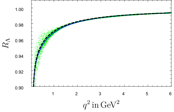
Figure 1: The q2q^{2}-dependence of RΛR_{\Lambda}. The blue solid line is found using the values of the form factors in covariant quark model given in Table 3. This line almost coincides with the estimate using SCET form factors plotted as a black dotted line. The green band represents the possible values of RΛR_{\Lambda} obtained by randomly generating 10410^{4} points corresponding to ±30%\pm 30\% error in each of the covariant quark model form factor estimates.

The decay rates for Λb→Λ​e+​e−\Lambda_{b}\to\Lambda e^{+}e^{-} and Λb→Λ​μ+​μ−\Lambda_{b}\to\Lambda\mu^{+}\mu^{-} can be readily calculated once the values of relevant form factors are fixed. Our interest lies primarily in low-q2q^{2} (high recoil) region i.e. q2=0.04​Ge​V2−6​Ge​V2q^{2}=0.04\mathrm{Ge\kern-1.00006ptV}^{2}-6\mathrm{Ge\kern-1.00006ptV}^{2} and it has been emphasized in  [58, 59, 60, 62, 61] that heavy-quark symmetry is not reliable at low-q2q^{2}. Heavy quark symmetry is expected to break down as one deviates from the zero-recoil point  [58, 59]. We, therefore, follow the approach of [19], which uses covariant quark model (CQM) to calculate the required form factors at low-q2q^{2}. We quote the values of those form factors [19] in Table 3 and calculate R⁡(Λ)R(\Lambda), the ratio of decay rates for Λb→Λ​μ+​μ−\Lambda_{b}\to\Lambda\mu^{+}\mu^{-} and Λb→Λ​e+​e−\Lambda_{b}\to\Lambda e^{+}e^{-}. We also, use Soft-collinear effective theory (SCET) and compare the two estimates obtained for the decay rate. A heavy-to-light transition of Λb\Lambda_{b} to Λ\Lambda in large recoil (low q2q^{2}) limit is simplified as the number of independent form factor reduces to one. SCET is valid  [63, 62] in this energy range as the energy of the daughter Λ\Lambda is larger than its mass and one can use the λ=mΛmb\lambda=\sqrt{\frac{m_{\Lambda}}{m_{b}}} as an expansion parameter which is small. In such a picture, the hadronic matrix elements in Eq. (15) for Λb→Λ\Lambda_{b}\to\Lambda decay can be parametrized in the following way,

⟨Λ⁡(p2)|s¯​Γ​b|Λb​(p)⟩≃ξλ​(E2)​u¯Λ​(p2)​Γ​uΛb​(p)+𝒪⁡(λ2​ξλ)\displaystyle\langle\Lambda(p_{2})|\bar{s}\Gamma b|\Lambda_{b}(p)\rangle\simeq\xi_{\lambda}(E_{2})\bar{u}_{\Lambda}(p_{2})\Gamma u_{\Lambda_{b}}(p)+\mathcal{O}(\lambda^{2}\xi_{\lambda})

To start with, let us highlight the relations between different form factors used in Eqn. (15) in low q2q^{2} limit,

f1V≈f1A≈−f2T​V≈−f2T​A=ξλ\displaystyle f_{1}^{V}\approx f_{1}^{A}\approx-f_{2}^{TV}\approx-f_{2}^{TA}=\xi_{\lambda} (31)
f2V≈f3V≈f2A≈f3A≈f1T​V≈f1T​A≈0\displaystyle f_{2}^{V}\approx f_{3}^{V}\approx f_{2}^{A}\approx f_{3}^{A}\approx f_{1}^{TV}\approx f_{1}^{TA}\approx 0 (32)

where ξλ\xi_{\lambda} is the single parameter all non-zero form factors depend on in the limit of small q2q^{2} [64, 63]. In Fig. 1, we have plotted R⁡(Λ)R(\Lambda). We have gone further and also probed the reliability of RΛR_{\Lambda} value by randomly adding ±30%\pm 30\% error to each form factor estimate in covariant quark model and by generating 10410^{4} points to evaluate the ratio. It is thus concluded that RΛR_{\Lambda} is reliably predicted in the low-q2q^{2} (high recoil) region of q2=0.04​Ge​V2−6​Ge​V2q^{2}=0.04\mathrm{Ge\kern-1.00006ptV}^{2}-6\mathrm{Ge\kern-1.00006ptV}^{2}. The contributions to RΛR_{\Lambda} from long-distance effects will be discussed later.

Figure 2: The q2q^{2}-dependence of the forward-backward asymmetries AF​BlA_{FB}^{l}, AF​BhA_{FB}^{h}, AF​Bh​lA_{FB}^{hl} for electron and muon are presented. For muons, the q2q^{2}-dependence of the asymmetries are given by the solid red line, obtained using covariant quark model form-factors and the blue dotted line is for SCET form factors. For electrons, the solid green line represents the q2q^{2}-dependence using covariant quark model form factors whereas the black dotted line represents the q2q^{2}-dependence due to SCET form factors.

IV.1 Angular Observables

In this section we list the angular asymmetries that allow us to extract the angular coefficients I2⋯I10I_{2}\cdots I_{10} and contribute to nine of the ten observables, with I1I_{1} being the total differential decay rate. These asymmetries result from orthogonal angular distribution and are thus independent observables.

A2\displaystyle A_{2} =[∫−1−12−∫−1212+∫121]dcosθl∫−11dcosθΛ∫02​πdϕ13​πd4​Γdq2dcosθΛdcosθldϕ∫−11dcosθl∫−11dcosθΛ∫02​πdϕd4​Γdq2dcosθΛdcosθldϕ\displaystyle=\frac{\displaystyle\Big[\int_{-1}^{-\frac{1}{2}}-\int_{-\frac{1}{2}}^{\frac{1}{2}}+\int_{\frac{1}{2}}^{1}\Big]d\cos\theta_{l}\int_{-1}^{1}d\cos\theta_{\Lambda}\int_{0}^{2\pi}d\phi\frac{1}{3\pi}\frac{d^{4}\Gamma}{dq^{2}d\cos\theta_{\Lambda}d\cos\theta_{l}d\phi}}{\displaystyle\int_{-1}^{1}d\cos\theta_{l}\int_{-1}^{1}d\cos\theta_{\Lambda}\int_{0}^{2\pi}d\phi\frac{d^{4}\Gamma}{dq^{2}d\cos\theta_{\Lambda}d\cos\theta_{l}d\phi}} (33)
A3\displaystyle A_{3} =[−∫−10+∫01]dcosθl∫−11dcosθΛ∫02​πdϕ14​πd4​Γdq2dcosθΛdcosθldϕ∫−11dcosθl∫−11dcosθΛ∫02​πdϕd4​Γdq2dcosθΛdcosθldϕ\displaystyle=\frac{\displaystyle\Big[-\int_{-1}^{0}+\int_{0}^{1}\Big]d\cos\theta_{l}\int_{-1}^{1}d\cos\theta_{\Lambda}\int_{0}^{2\pi}d\phi\frac{1}{4\pi}\frac{d^{4}\Gamma}{dq^{2}d\cos\theta_{\Lambda}d\cos\theta_{l}d\phi}}{\displaystyle\int_{-1}^{1}d\cos\theta_{l}\int_{-1}^{1}d\cos\theta_{\Lambda}\int_{0}^{2\pi}d\phi\frac{d^{4}\Gamma}{dq^{2}d\cos\theta_{\Lambda}d\cos\theta_{l}d\phi}} (34)
A4\displaystyle A_{4} =∫−11dcosθl[−∫−10+∫01]dcosθΛ∫02​πdϕ14​πd4​Γdq2dcosθΛdcosθldϕ∫−11dcosθl∫−11dcosθΛ∫02​πdϕd4​Γdq2dcosθΛdcosθldϕ\displaystyle=\frac{\displaystyle\int_{-1}^{1}d\cos\theta_{l}\Big[-\int_{-1}^{0}+\int_{0}^{1}\Big]d\cos\theta_{\Lambda}\int_{0}^{2\pi}d\phi\frac{1}{4\pi}\frac{d^{4}\Gamma}{dq^{2}d\cos\theta_{\Lambda}d\cos\theta_{l}d\phi}}{\displaystyle\int_{-1}^{1}d\cos\theta_{l}\int_{-1}^{1}d\cos\theta_{\Lambda}\int_{0}^{2\pi}d\phi\frac{d^{4}\Gamma}{dq^{2}d\cos\theta_{\Lambda}d\cos\theta_{l}d\phi}} (35)
A5\displaystyle A_{5} =43​[−∫−1−12+∫−1212−∫121]dcosθl[∫−10−∫01]dcosθΛ∫02​πdϕd4​Γdq2dcosθΛdcosθldϕ∫−11dcosθl∫−11dcosθΛ∫02​πdϕd4​Γdq2dcosθΛdcosθldϕ\displaystyle=\frac{4}{3}\frac{\displaystyle\Big[-\int_{-1}^{-\frac{1}{2}}+\int_{-\frac{1}{2}}^{\frac{1}{2}}-\int_{\frac{1}{2}}^{1}\Big]d\cos\theta_{l}\Big[\int_{-1}^{0}-\int_{0}^{1}\Big]d\cos\theta_{\Lambda}\int_{0}^{2\pi}d\phi\frac{d^{4}\Gamma}{dq^{2}d\cos\theta_{\Lambda}d\cos\theta_{l}d\phi}}{\displaystyle\int_{-1}^{1}d\cos\theta_{l}\int_{-1}^{1}d\cos\theta_{\Lambda}\int_{0}^{2\pi}d\phi\frac{d^{4}\Gamma}{dq^{2}d\cos\theta_{\Lambda}d\cos\theta_{l}d\phi}} (36)
A6\displaystyle A_{6} =[∫−10−∫01]dcosθl[∫−10−∫01]dcosθΛ∫02​πdϕd4​Γdq2dcosθΛdcosθldϕ∫−11dcosθl∫−11dcosθΛ∫02​πdϕd4​Γdq2dcosθΛdcosθldϕ\displaystyle=\frac{\displaystyle\Big[\int_{-1}^{0}-\int_{0}^{1}\Big]d\cos\theta_{l}\Big[\int_{-1}^{0}-\int_{0}^{1}\Big]d\cos\theta_{\Lambda}\int_{0}^{2\pi}d\phi\frac{d^{4}\Gamma}{dq^{2}d\cos\theta_{\Lambda}d\cos\theta_{l}d\phi}}{\displaystyle\int_{-1}^{1}d\cos\theta_{l}\int_{-1}^{1}d\cos\theta_{\Lambda}\int_{0}^{2\pi}d\phi\frac{d^{4}\Gamma}{dq^{2}d\cos\theta_{\Lambda}d\cos\theta_{l}d\phi}} (37)
A7\displaystyle A_{7} =−34​[∫−10−∫01]dcosθl∫−11dcosθΛ[∫−π2π2−∫π23​π2]dϕd4​Γdq2dcosθΛdcosθldϕ∫−11dcosθl∫−11dcosθΛ∫02​πdϕd4​Γdq2dcosθΛdcosθldϕ\displaystyle=-\frac{3}{4}\frac{\displaystyle\Big[\int_{-1}^{0}-\int_{0}^{1}\Big]d\cos\theta_{l}\int_{-1}^{1}d\cos\theta_{\Lambda}\Big[\int_{\frac{-\pi}{2}}^{\frac{\pi}{2}}-\int_{\frac{\pi}{2}}^{\frac{3\pi}{2}}\Big]d\phi\frac{d^{4}\Gamma}{dq^{2}d\cos\theta_{\Lambda}d\cos\theta_{l}d\phi}}{\displaystyle\int_{-1}^{1}d\cos\theta_{l}\int_{-1}^{1}d\cos\theta_{\Lambda}\int_{0}^{2\pi}d\phi\frac{d^{4}\Gamma}{dq^{2}d\cos\theta_{\Lambda}d\cos\theta_{l}d\phi}} (38)
A8\displaystyle A_{8} =∫−11dcosθl∫−11dcosθΛ[−∫−π−π2+∫−π2π2−∫π2π]dϕd4​Γdq2dcosθΛdcosθldϕ∫−11dcosθl∫−11dcosθΛ∫02​πdϕd4​Γdq2dcosθΛdcosθldϕ\displaystyle=\frac{\displaystyle\int_{-1}^{1}d\cos\theta_{l}\int_{-1}^{1}d\cos\theta_{\Lambda}\Big[-\int_{-\pi}^{\frac{-\pi}{2}}+\int_{\frac{-\pi}{2}}^{\frac{\pi}{2}}-\int_{\frac{\pi}{2}}^{\pi}\Big]d\phi\frac{d^{4}\Gamma}{dq^{2}d\cos\theta_{\Lambda}d\cos\theta_{l}d\phi}}{\displaystyle\int_{-1}^{1}d\cos\theta_{l}\int_{-1}^{1}d\cos\theta_{\Lambda}\int_{0}^{2\pi}d\phi\frac{d^{4}\Gamma}{dq^{2}d\cos\theta_{\Lambda}d\cos\theta_{l}d\phi}} (39)
A9\displaystyle A_{9} =−34​[∫−10−∫01]dcosθl∫−11dcosθΛ[∫0π−∫π2​π]dϕd4​Γdq2dcosθΛdcosθldϕ∫−11dcosθl∫−11dcosθΛ∫02​πdϕd4​Γdq2dcosθΛdcosθldϕ\displaystyle=-\frac{3}{4}\frac{\Big[\displaystyle\int_{-1}^{0}-\int_{0}^{1}\Big]d\cos\theta_{l}\int_{-1}^{1}d\cos\theta_{\Lambda}\Big[\int_{0}^{\pi}-\int_{\pi}^{2\pi}\Big]d\phi\frac{d^{4}\Gamma}{dq^{2}d\cos\theta_{\Lambda}d\cos\theta_{l}d\phi}}{\displaystyle\int_{-1}^{1}d\cos\theta_{l}\int_{-1}^{1}d\cos\theta_{\Lambda}\int_{0}^{2\pi}d\phi\frac{d^{4}\Gamma}{dq^{2}d\cos\theta_{\Lambda}d\cos\theta_{l}d\phi}} (40)
A10\displaystyle A_{10} =1π2​∫−11dcosθl∫−11dcosθΛ[∫−π0+∫0π]dϕd4​Γdq2dcosθΛdcosθldϕ∫−11dcosθl∫−11dcosθΛ∫02​πdϕd4​Γdq2dcosθΛdcosθldϕ\displaystyle=\frac{1}{\pi^{2}}\frac{\displaystyle\int_{-1}^{1}d\cos\theta_{l}\int_{-1}^{1}d\cos\theta_{\Lambda}\Big[\int_{-\pi}^{0}+\int_{0}^{\pi}\Big]d\phi\frac{d^{4}\Gamma}{dq^{2}d\cos\theta_{\Lambda}d\cos\theta_{l}d\phi}}{\displaystyle\int_{-1}^{1}d\cos\theta_{l}\int_{-1}^{1}d\cos\theta_{\Lambda}\int_{0}^{2\pi}d\phi\frac{d^{4}\Gamma}{dq^{2}d\cos\theta_{\Lambda}d\cos\theta_{l}d\phi}}\ (41)

Note that A9A_{9} and A10A_{10} are non-zero only if the amplitudes have imaginary contributions. These are expected to be extremely tiny in the SM. The asymmetries A2A_{2}, A5A_{5}, A7A_{7} and A8A_{8} are not simple forward back asymmetries. We note that A3A_{3}, A4A_{4} are forward-backward asymmetries in the leptonic angle θl\theta_{l} and hadronic angle θΛ\theta_{\Lambda} respectively. There is also a double asymmetry involving θl\theta_{l} and θΛ\theta_{\Lambda} given by A6A_{6}. We provide an expression for each of these quantities in terms of known parameters.

Refer to caption
Refer to caption
Refer to caption
Figure 3: The q2q^{2} dependence for the ratios of forward-backward asymmetries RAF​BlR_{A_{FB}^{l}}, RAF​BhR_{A_{FB}^{h}} and RAF​Bh​lR_{A_{FB}^{hl}} (see Eqs. (50)–(52)). The blue solid line is found using the values of form factors in covariant quark model given in Table 3. This line almost coincides with the estimate using SCET form factors, represented as the black dotted line. Note that, while the two asymmetries AF​B,μhA_{FB,\mu}^{h} and AF​B,ehA_{FB,e}^{h} are form factor dependent the ratio RAF​BhR_{A_{FB}^{h}} is independent of the choice of form-factors (CQM or SCET). The green band represents the possible values of RΛR_{\Lambda} obtained by randomly generating 10410^{4} points corresponding to ±30%\pm 30\% error in each of the covariant quark model form factor estimates.
AF​Bl\displaystyle A^{l}_{FB} =\displaystyle= −3vRe[A∗L⟂,1AL∥,1−(L↔R)]q24​I1\displaystyle\displaystyle\frac{-3v\ \text{Re}\big[A^{*L}_{\perp,1}A^{L}_{\parallel,1}-\big(L\leftrightarrow R\big)\big]q^{2}}{4I_{1}} (42)
AF​Bh\displaystyle A^{h}_{FB} =\displaystyle= αΛ​[(1−mℓ2q2)Re{A∗L⟂,0AL∥,0+A∗L⟂,1AL∥,1+(L↔R)}+3​mℓ2q2Re{A∗t,∥At,⟂}+3​mℓ2q2{Re(A∗R⟂,0AL∥,0+A∗L⟂,0AR∥,0+A∗R⟂,1AL∥,1+A∗L⟂,1AR∥,1)}]​q22​I1\displaystyle\displaystyle\frac{\displaystyle\alpha_{\Lambda}\Bigg[\begin{multlined}(1-\frac{m_{\ell}^{2}}{q^{2}})\text{Re}\Big\{A^{*L}_{\perp,0}A^{L}_{\parallel,0}+A^{*L}_{\perp,1}A^{L}_{\parallel,1}+\big(L\leftrightarrow R\big)\Big\}+\frac{3m_{\ell}^{2}}{q^{2}}\text{Re}\{A^{*}_{t,\parallel}A_{t,\perp}\}\\ \\ \displaystyle+\frac{3m_{\ell}^{2}}{q^{2}}\big\{\text{Re}(A^{*R}_{\perp,0}A^{L}_{\parallel,0}+A^{*L}_{\perp,0}A^{R}_{\parallel,0}+A^{*R}_{\perp,1}A^{L}_{\parallel,1}+A^{*L}_{\perp,1}A^{R}_{\parallel,1})\big\}\end{multlined}\Bigg]q^{2}}{{2I_{1}}}
AF​Bh​l\displaystyle A^{hl}_{FB} =\displaystyle= −3vαΛ[|AL∥,1|2+|AL⟂,1|2−(L↔R)]q28​I1\displaystyle\displaystyle\frac{-3v\alpha_{\Lambda}\Big[|A^{L}_{\parallel,1}|^{2}+|A^{L}_{\perp,1}|^{2}-\big(L\leftrightarrow R\big)\Big]q^{2}}{8I_{1}} (47)
Refer to caption
Refer to caption
Refer to caption
Refer to caption
Figure 4: The q2q^{2} dependence of the ratios of other observables R2,R5,R7,R8R_{2},\,R_{5},\,R_{7},\,R_{8} that are not simple forward-backward asymmetries (See Eqn 53-56). The color code is the same as in Fig 3.

.

AF​BlA_{FB}^{l}, AF​BhA_{FB}^{h}, AF​Bh​lA_{FB}^{hl} are lepton side forward-backward asymmetry, hadron side forward backward asymmetry and double forward-backward asymmetry respectively. The parameter αΛ\alpha_{\Lambda} is the asymmetry parameter of the decay Λ→p+​π−\Lambda\rightarrow p^{+}\pi^{-} which is defined as,

αΛ=βτ=|h−12,0|2−|h12,0|2|h−12,0|2+|h12,0|2\displaystyle\alpha_{\Lambda}=\frac{\beta}{\tau}=\frac{|h_{-\frac{1}{2},0}|^{2}-|h_{\frac{1}{2},0}|^{2}}{|h_{-\frac{1}{2},0}|^{2}+|h_{\frac{1}{2},0}|^{2}} (48)

Note that the convention used by us is same as in [19] upto an overall negative sign. The asymmetry parameter has been measured to be αΛ=0.642±0.013\alpha_{\Lambda}=0.642\pm 0.013 [65]. As mentioned already, this is in contrast to the mesonic counterpart B→K∗(→Kπ)ℓ+ℓ−B\rightarrow K^{*}(\rightarrow K\pi)\ell^{+}\ell^{-}, where the subsequent K∗→K​πK^{*}\rightarrow K\pi decay is parity conserving and thus no forward-backward asymmetry in the hadronic angle θK∗\theta_{K^{*}} is observed. While we are discussing AF​BhA_{FB}^{h} we would also like to point out that it is sensitive to the timelike polarization of jeff j_{{\text{eff }}} as the presence of AtA_{t} can be seen in Eq. (IV.1). If we are to restrict ourselves to the SM effective operators, the transversity amplitude AtA_{t} involves the Wilson coefficient C10C_{10} only. AtA_{t} receives additional contribution in presence of pseudoscalar operators of the form (s¯​γ5​b)​(l​γ5​l)\left(\bar{s}\gamma_{5}b\right)(l\gamma_{5}l) as shown in [5]. Thus, AF​BhA_{FB}^{h} provides an independent test of pseudoscalar currents that are not present in the SM. The lepton forward-backward asymmetry is given by AF​BlA^{l}_{FB}, which depends on the real part of the interference between two amplitudes A⟂,1A_{\perp,1} and A∥,1A_{\parallel,1}. The presence of the factor vv suggests that lepton forward-backward asymmetry vanishes as q2→4​ml2q^{2}\rightarrow 4m_{l}^{2}. The double forward-backward asymmetry is given by AF​Bh​lA_{FB}^{hl}. It is clear that AF​Bh​lA_{FB}^{hl} vanishes when either asymmetry parameter αΛ=0\alpha_{\Lambda}=0 or q2→4​ml2q^{2}\rightarrow 4m_{l}^{2}.

An interesting feature of the three forward-backward observables AF​BlA_{FB}^{l}, AF​BhA_{FB}^{h} and AF​Bh​lA_{FB}^{hl} is their characteristic-q2q^{2} dependence. More precisely, within the SM one finds that both AF​BlA_{FB}^{l} and AF​Bh​lA_{FB}^{hl} cross zero, in contrast to AF​BhA_{FB}^{h} which doesn’t. Moreover, to the leading order, the zero crossing points are same for AF​BlA_{FB}^{l} and AF​Bh​lA_{FB}^{hl}. The q02q_{0}^{2} value only depends on ratios of Wilson coefficients, a result well known from other exclusive and inclusive b→s​ℓ+​ℓ−b\to s\ell^{+}\ell^{-} decay, and to leading order,

q02≈−2​mb​mΛb​C7C9\displaystyle q^{2}_{0}\approx-\frac{2m_{b}m_{\Lambda_{b}}C_{7}}{C_{9}} (49)

If we relax the assumption that Wilson coefficients to be flavor blind and allow for the possibility of C9μ≠C9eC_{9}^{\mu}\neq C_{9}^{e}, then the zero crossing point will be different for muon and electron. Thus, by observing q02q_{0}^{2}, the zero crossing values for observables like AF​BeA_{FB}^{e} and AF​BμA_{FB}^{\mu}, one can extract vital information about the underlying flavor structure of the theory. There are also other theoretically clean observables having zero crossing point in large-q2q^{2} region as emphasized in Ref [22]. Thus, a careful study of the zero crossing points of these observables is necessary over the whole q2q^{2} range to disentangle genuine new physics contribution, which is expected to be q2q^{2} independent, from any unaccounted hadronic effects.

We construct ratios of AF​BμA_{FB}^{\mu}, AF​B,μhA_{FB,\mu}^{h}, AF​Bh​μA_{FB}^{h\mu} to the corresponding quantities for the electron i.e. AF​BeA_{FB}^{e}, AF​B,ehA_{FB,e}^{h}, AF​Bh​eA_{FB}^{he}. These ratios are defined in a similar vein as done in  [66, 67, 68, 69],

R3=RAF​Bl\displaystyle R_{3}=R_{A_{FB}^{l}} =AF​BμAF​Be\displaystyle=\frac{A_{FB}^{\mu}}{A_{FB}^{e}} (50)
R4=RAF​Bh\displaystyle R_{4}=R_{A_{FB}^{h}} =AF​B,μhAF​B,eh\displaystyle=\frac{A_{FB,\mu}^{h}}{A_{FB,e}^{h}} (51)
R6=RAF​Bh​l\displaystyle R_{6}=R_{A_{FB}^{hl}} =AF​B,μh​lAF​B,eh​l.\displaystyle=\frac{A_{FB,\mu}^{hl}}{A_{FB,e}^{hl}}. (52)

We additionally provide here ratios of other angular observables for muons namely A2μA_{2}^{\mu}, A5μA_{5}^{\mu}, A7μA_{7}^{\mu}, A8μA_{8}^{\mu} to the corresponding quantities for the electrons.

R2=A2μA2e\displaystyle R_{2}=\frac{A_{2}^{\mu}}{A_{2}^{e}} (53)
R5=A5μA5e\displaystyle R_{5}=\frac{A_{5}^{\mu}}{A_{5}^{e}} (54)
R7=A7μA7e\displaystyle R_{7}=\frac{A_{7}^{\mu}}{A_{7}^{e}} (55)
R8=A8μA8e\displaystyle R_{8}=\frac{A_{8}^{\mu}}{A_{8}^{e}} (56)

A natural question that arises is “to what extent the ratios defined in Eqn.(42)-(47) deviate from the case where individual form factors are only known to a certain accuracy.” In SCET the helicity amplitudes defined in Eqn.(22) are expressible in terms of the parameter ξλ\xi_{\lambda}. This simplification leads to ξλ\xi_{\lambda} getting factored out and it cancels when ratios like AF​BlA_{FB}^{l}, AF​BhA_{FB}^{h}, AF​Bh​lA_{FB}^{hl} are defined. In Fig. 2 we plot the AF​BlA_{FB}^{l}, AF​BhA_{FB}^{h}, AF​Bh​lA_{FB}^{hl} for the case of ℓ=e\ell=e and ℓ=μ\ell=\mu separately in the low q2q^{2} region. There is however dependence on form-factor in the observable of especial interest, the hadronic forward-backward asymmetry AF​B,lhA_{FB,l}^{h} as can be seen in Fig. 2. Fortunately it turns out that the dependence on choice of form-factors cancels out in the ratios of asymmetries defined as RAF​BlR_{A_{FB}^{l}}, RAF​BhR_{A_{FB}^{h}} and RAF​Bh​lR_{A_{FB}^{hl}}. Nevertheless, if the measurement of these ratios differ from the predicted ones, one may question the accuracy of form-factors which are only calculated based on a model. In order to ascertain the sensitivity of these ratios due to inaccuracies in the form factors, we randomly add ±30%\pm 30\% error to each form factor estimates in covariant quark model and generate 10410^{4} points to evaluate the ratios RAF​BlR_{A_{FB}^{l}}, RAF​BhR_{A_{FB}^{h}} and RAF​Bh​lR_{A_{FB}^{hl}}. In Fig. 3, we have plotted these ratios RAF​BlR_{A_{FB}^{l}}, RAF​BlR_{A_{FB}^{l}} and RAF​Bh​lR_{A_{FB}^{hl}}. In contrast to RAF​BlR_{A_{FB}^{l}} and RAF​Bh​lR_{A_{FB}^{hl}}, RAF​BhR_{A_{FB}^{h}} is a ratio of two non-vanishing asymmetries at low-q2q^{2}, hence, it is likely to be more accurately measured. The ratio of the remaining angular observables defined in Eqn.(53)-(56) are plotted in Fig. 4. We conclude this section by providing a numerical estimate of the ratios RΛR_{\Lambda}, RAF​BlR_{A_{FB}^{l}}, RAF​BhR_{A_{FB}^{h}} in Table  4 for two q2q^{2}-integrated bins. All the ratios show a remarkable insensitivity to the form factor uncertainties. In the above analysis we have not considered the contribution from long-distance effects. However, this is unlikely to affect our conclusions based on a recent study [70] of long-distance effects in the analogous mode B→K∗​μ+​μ−B\to K^{*}\mu^{+}\mu^{-}. It has been shown in Ref. [70] that RK∗R_{K^{\!*}} is insensitive to long distance effects within the realm of SM.

Binned Ratios Bin 1 Bin 2
q2∼q^{2}\sim 0.045-1Ge​V\mathrm{Ge\kern-1.00006ptV}2 q2∼q^{2}\sim 1-6Ge​V\mathrm{Ge\kern-1.00006ptV}2
RΛR_{\Lambda} 0.907±\pm 0.003 0.9885 ±\pm 0.0002
RAF​BlR_{A^{l}_{FB}} 0.9469 ±\pm 0.0007 0.998±\pm0.196
RAF​BhR_{A^{h}_{FB}} 0.993±\pm0.001 >0.9973>0.9973 (0.9990.999%C.L.)
Table 4: The binned values of the observables RΛR_{\Lambda}, RAF​BlR_{A_{FB}^{l}}, RAF​BhR_{A_{FB}^{h}}. Only RAF​BhR_{A_{FB}^{h}} for q2∼q^{2}\sim 1-6 Ge​V\mathrm{Ge\kern-1.00006ptV}2 does not show a Gaussian behavior as it is peaked towards unity.

V Conclusions

The baryonic decay mode Λb→Λ​ℓ+​ℓ−\Lambda_{b}\rightarrow\Lambda\ell^{+}\ell^{-} is similar at the quark level to the much studied mesonic decay mode B→K∗​ℓ+​ℓ−B\to{K^{\!*}}\ell^{+}\ell^{-} and is hence, also expected to provide a plethora of observables that can be used to probe NP and better understand the hadronic effects accompanying the weak decay. While this mode has been a subject of several studies, we have reexamined the decay mode with focus on aspects that have not been studied in detail earlier. We have derived the angular distribution without any approximations. In particular, we retain the finite lepton mass effects and the two time like amplitudes. These contributions play a significant role in estimating accurately the size of lepton non-universality that may show up in the mode within SM. We estimate RΛR_{\Lambda} which is defined in a manner identical to RK(∗)R_{K^{\!(\!*\!)}} [see Eqs. (1) and (2)]. The non-zero lepton mass effects become increasingly important in low-q2q^{2} region where the discrepancy between SM expectation and the experimentally observed value of RK(∗)R_{K^{\!(\!*\!)}} is largest. The observation of a similar discrepancy in RΛR_{\Lambda} is therefore necessary to substantiate the idea of lepton non-universality in FCNC processes since such observations cannot be restricted to the B→K(∗)​ℓ+​ℓ−B\rightarrow K^{(*)}\ell^{+}\ell^{-} alone. A discrepancy between the estimates presented here and upcoming measurements at LHCb, would establish that the existence of non-universality in interactions involving fermions on firm footing.

The angular distribution of the decay products in Λb→Λ(→p+π−)ℓ+ℓ−\Lambda_{b}\rightarrow\Lambda(\rightarrow p^{+}\pi^{-})\ell^{+}\ell^{-} decay, provides a wealth of information on the nature of decay. This is characterized by the angular observables expressed in terms of helicity amplitudes. We have presented a complete set of ten angular observables that can be measured using this decay mode. We study in detail the three forward-backward asymmetries AF​BlA_{FB}^{l}, AF​BhA_{FB}^{h} and AF​Bh​lA_{FB}^{hl}. It may be noted that no hadron angle forward-back asymmetry exists for the mode B→K∗​ℓ+​ℓ−B\to{K^{\!*}}\ell^{+}\ell^{-}. The asymmetry AF​BhA_{FB}^{h} is found to be especially interesting since it is non-vanishing in the large recoil limit, unlike the case with B→K∗​ℓ+​ℓ−B\to{K^{\!*}}\ell^{+}\ell^{-} decay mode, where all asymmetries vanish in the low-q2q^{2} limit. This is a consequence of the parity violating nature of the subsequent Λ→p​π\Lambda\to p\pi decay. The non-vanishing asymmetry is particularly sensitive to new physics that violates lepton flavor universality, since it involves comparing two finite quantities for the cases of ℓ=μ\ell=\mu and ℓ=e\ell=e respectively. It may be noted that all the asymmetries in B→K∗​ℓ+​ℓ−B\to K^{*}\ell^{+}\ell^{-} vanish in the low-q2q^{2} limit and as such result in comparisons between two vanishing quantities.

We numerically estimate the three asymmetries AF​BlA_{FB}^{l}, AF​BhA_{FB}^{h} and AF​Bh​lA_{FB}^{hl} and the ratios RΛR_{\Lambda}, RAF​BlR_{A_{FB}^{l}}, RAF​BhR_{A_{FB}^{h}}, RAF​Bh​lR_{A_{FB}^{hl}}. In order to ascertain that our results are not very sensitive to the choice of form-factors we use two different approaches to form factors. We have used both the covariant quark model and soft-collinear effective theory to calculate all the observables. We find that all above mentioned ratios are remarkably insensitive to the choice of factors as can be seen from Fig. 1 and Fig. 4. In order to probe the reliability of the values estimated for these ratios we have randomly added ±30%\pm 30\% error to each form factor estimates in covariant quark model to evaluate these ratios as well. In contrast to RAF​BlR_{A_{FB}^{l}} and RAF​Bh​lR_{A_{FB}^{hl}}, RAF​BhR_{A_{FB}^{h}} is a ratio of two non-vanishing asymmetries at low-q2q^{2}, hence, it is likely to be more accurately measured. We have numerically estimated the ratios RΛR_{\Lambda}, RAF​BlR_{A_{FB}^{l}}, RAF​BhR_{A_{FB}^{h}} in two q2q^{2}-integrated bins. All the ratios show a remarkable insensitivity to the form factor uncertainties. Since these ratios are expected to be insensitive [70] to long-distance contributions, we conclude that, RΛR_{\Lambda} and RAF​BhR_{A_{FB}^{h}} are both experimentally and theoretically reliable observables to test new physics beyond the standard model.

References

  • [1] D. Das and R. Sinha, Phys. Rev. D 86, 056006 (2012) [arXiv:1205.1438 [hep-ph]].
  • [2] R. Mandal, R. Sinha and D. Das, Phys. Rev. D 90, no. 9, 096006 (2014) [arXiv:1409.3088 [hep-ph]].
  • [3] R. Mandal and R. Sinha, Phys. Rev. D 95, no. 1, 014026 (2017) [arXiv:1506.04535 [hep-ph]].
  • [4] F. Kruger and J. Matias, Phys. Rev. D 71, 094009 (2005) [hep-ph/0502060].
  • [5] W. Altmannshofer, P. Ball, A. Bharucha, A. J. Buras, D. M. Straub and M. Wick, JHEP 0901, 019 (2009) [arXiv:0811.1214 [hep-ph]].
  • [6] C. Bobeth, G. Hiller and G. Piranishvili, JHEP 0807, 106 (2008) [arXiv:0805.2525 [hep-ph]].
  • [7] U. Egede, T. Hurth, J. Matias, M. Ramon and W. Reece, JHEP 0811, 032 (2008) [arXiv:0807.2589 [hep-ph]].
  • [8] C. Bobeth, G. Hiller and D. van Dyk, JHEP 1007, 098 (2010) [arXiv:1006.5013 [hep-ph]].
  • [9] D. Becirevic and E. Schneider, Nucl. Phys. B 854, 321 (2012) [arXiv:1106.3283 [hep-ph]].
  • [10] C. Bobeth, G. Hiller and D. van Dyk, Phys. Rev. D 87, no. 3, 034016 (2013) [Phys. Rev. D 87, 034016 (2013)] [arXiv:1212.2321 [hep-ph]].
  • [11] G. Hiller and R. Zwicky, JHEP 1403, 042 (2014) [arXiv:1312.1923 [hep-ph]].
  • [12] J. Gratrex, M. Hopfer and R. Zwicky, Phys. Rev. D 93, no. 5, 054008 (2016) [arXiv:1506.03970 [hep-ph]].
  • [13] B. Grinstein and D. Pirjol, Phys. Rev. D 70, 114005 (2004) [hep-ph/0404250].
  • [14] W. Altmannshofer and D. M. Straub, Eur. Phys. J. C 73, 2646 (2013) [arXiv:1308.1501 [hep-ph]].
  • [15] R. Aaij et al. [LHCb Collaboration], Phys. Rev. Lett. 111, 191801 (2013) [arXiv:1308.1707 [hep-ex]].
  • [16] S. Chatrchyan et al. [CMS Collaboration], Phys. Lett. B 727, 77 (2013) [arXiv:1308.3409 [hep-ex]].
  • [17] Other observed signals of lepton non-universality are a consequence of τ\tau versus ℓ={μ,e}\ell=\{\mu,e\} non-universality given by the measurement of R⁡(D(∗))=BR⁡(B→D(∗)​τ​ν)BR⁡(B→D(∗)​ℓ​ν)R(D^{(*)})=\frac{{\rm BR}(B\to D^{(*)}\tau\nu)}{{\rm BR}(B\to D^{(*)}\ell\nu)}. Very recently LHCb has reported similar discrepancy in R⁡(J/ψ)=BR⁡(B→J/ψ​τ​ν)BR⁡(B→J/ψ​ℓ​ν)R(J\!/\!\psi)=\frac{{\rm BR}(B\to J\!/\!\psi\tau\nu)}{{\rm BR}(B\to J\!/\!\psi\ell\nu)}[arXiv:1711.05623[hep-ex]].
  • [18] T. Gutsche, M. A. Ivanov, J. G. Körner, V. E. Lyubovitskij and P. Santorelli, Phys. Rev. D 88, no. 11, 114018 (2013) [arXiv:1309.7879 [hep-ph]].
  • [19] T. Gutsche, M. A. Ivanov, J. G. Körner, V. E. Lyubovitskij and P. Santorelli, Phys. Rev. D 87, 074031 (2013) [arXiv:1301.3737 [hep-ph]].
  • [20] P. Böer, T. Feldmann and D. van Dyk, JHEP 1501, 155 (2015) [arXiv:1410.2115 [hep-ph]].
  • [21] L. Mott and W. Roberts, Int. J. Mod. Phys. A 27, 1250016 (2012) [arXiv:1108.6129 [nucl-th]].
  • [22] G. Kumar and N. Mahajan, arXiv:1511.00935 [hep-ph].
  • [23] O. Leitner, Z. J. Ajaltouni and E. Conte, hep-ph/0602043.
  • [24] C. H. Chen and C. Q. Geng, Phys. Rev. D 64 (2001) 074001 [hep-ph/0106193].
  • [25] C. S. Huang and H. G. Yan, Phys. Rev. D 59, 114022 (1999) Erratum: [Phys. Rev. D 61, 039901 (2000)] [hep-ph/9811303].
  • [26] C. H. Chen and C. Q. Geng, Phys. Rev. D 63, 114024 (2001) [hep-ph/0101171].
  • [27] C. H. Chen and C. Q. Geng, Phys. Lett. B 516, 327 (2001) [hep-ph/0101201].
  • [28] T. M. Aliev, A. Ozpineci and M. Savci, Phys. Rev. D 65, 115002 (2002) [hep-ph/0203045].
  • [29] T. M. Aliev, A. Ozpineci, M. Savci and C. Yuce, Phys. Lett. B 542, 229 (2002) [hep-ph/0206014].
  • [30] T. M. Aliev, A. Ozpineci and M. Savci, Phys. Rev. D 67, 035007 (2003) [hep-ph/0211447].
  • [31] T. M. Aliev, V. Bashiry and M. Savci, Eur. Phys. J. C 38, 283 (2004) [hep-ph/0409275].
  • [32] A. K. Giri and R. Mohanta, J. Phys. G 31, 1559 (2005).
  • [33] T. M. Aliev and M. Savci, Eur. Phys. J. C 50, 91 (2007) [hep-ph/0606225].
  • [34] T. M. Aliev, M. Savci and B. B. Sirvanli, Eur. Phys. J. C 52, 375 (2007) [hep-ph/0608143].
  • [35] F. Zolfagharpour and V. Bashiry, Nucl. Phys. B 796, 294 (2008) [arXiv:0707.4337 [hep-ph]].
  • [36] M. J. Aslam, Y. M. Wang and C. D. Lu, Phys. Rev. D 78, 114032 (2008) [arXiv:0808.2113 [hep-ph]].
  • [37] Y. M. Wang, Y. Li and C. D. Lu, Eur. Phys. J. C 59, 861 (2009) [arXiv:0804.0648 [hep-ph]].
  • [38] Y. M. Wang, Y. L. Shen and C. D. Lu, Phys. Rev. D 80, 074012 (2009) [arXiv:0907.4008 [hep-ph]].
  • [39] T. M. Aliev, K. Azizi and M. Savci, Phys. Rev. D 81, 056006 (2010) [arXiv:1001.0227 [hep-ph]].
  • [40] S. Sahoo, C. K. Das and L. Maharana, Int. J. Mod. Phys. A 24, 6223 (2009) [arXiv:1112.4563 [hep-ph]].
  • [41] Y. M. Wang and Y. L. Shen, JHEP 1602, 179 (2016) [arXiv:1511.09036 [hep-ph]].
  • [42] T. Gutsche, M. A. Ivanov, J. G. K�rner, V. E. Lyubovitskij, V. V. Lyubushkin and P. Santorelli, Phys. Rev. D 96, no. 1, 013003 (2017) [arXiv:1705.07299 [hep-ph]].
  • [43] W. Detmold and S. Meinel, Phys. Rev. D 93, no. 7, 074501 (2016) [arXiv:1602.01399 [hep-lat]].
  • [44] S. Meinel and D. van Dyk, Phys. Rev. D 94, no. 1, 013007 (2016) [arXiv:1603.02974 [hep-ph]].
  • [45] R. N. Faustov and V. O. Galkin, Phys. Rev. D 96, no. 5, 053006 (2017) [arXiv:1705.07741 [hep-ph]].
  • [46] T. Blake and M. Kreps, JHEP 1711, 138 (2017) doi:10.1007/JHEP11(2017)138 [arXiv:1710.00746 [hep-ph]].
  • [47] R. Aaij et al. [LHCb Collaboration], JHEP 1708, 055 (2017) [arXiv:1705.05802 [hep-ex]].
  • [48] S. Bifani (on behalf of the LHCb Collab.), CERN seminar on April 18, 2017.
  • [49] R. Aaij et al. [LHCb Collab.], Phys. Rev. Lett. 113, 151601 (2014).
  • [50] G. Hiller and F. Kruger, Phys. Rev. D 69, 074020 (2004);
  • [51] A. Kadeer, J. G. Korner and U. Moosbrugger, Eur. Phys. J. C 59, 27 (2009) [hep-ph/0511019].
  • [52] T. Gutsche, M. A. Ivanov, J. G. Körner, V. E. Lyubovitskij, P. Santorelli and N. Habyl, Phys. Rev. D 91, no. 7, 074001 (2015) Erratum: [Phys. Rev. D 91, no. 11, 119907 (2015)] [arXiv:1502.04864 [hep-ph]].
  • [53] S. U. Chung, CERN-71-08.
  • [54] P. Bialas, J. G. Körner, M. Kramer and K. Zalewski, Z. Phys. C 57, 115 (1993).
  • [55] J. D. Richman, CALT-68-1148.
  • [56] J. G. Körner, arXiv:1402.2787 [hep-ph].
  • [57] G. Buchalla, A. J. Buras and M. E. Lautenbacher, Rev. Mod. Phys. 68, 1125 (1996) [hep-ph/9512380].
  • [58] J. G. Körner and P. Kroll, Z. Phys. C 57, 383 (1993).
  • [59] J. G. Körner and P. Kroll, Phys. Lett. B 293, 201 (1992).
  • [60] N. Isgur, Phys. Rev. D 43, 810 (1991).
  • [61] H. G. Dosch, E. Ferreira, M. Nielsen and R. Rosenfeld, Phys. Lett. B 431, 173 (1998) [hep-ph/9712350].
  • [62] T. Mannel and Y. M. Wang, JHEP 1112, 067 (2011) [arXiv:1111.1849 [hep-ph]].
  • [63] W. Wang, Phys. Lett. B 708, 119 (2012) [arXiv:1112.0237 [hep-ph]].
  • [64] T. Feldmann and M. W. Y. Yip, Phys. Rev. D 85, 014035 (2012) Erratum: [Phys. Rev. D 86, 079901 (2012)] [arXiv:1111.1844 [hep-ph]].
  • [65] J. Beringer et al. [Particle Data Group], Phys. Rev. D 86, 010001 (2012).
  • [66] B. Capdevila, S. Descotes-Genon, J. Matias and J. Virto, JHEP 1610, 075 (2016) [arXiv:1605.03156 [hep-ph]].
  • [67] S. Descotes-Genon, L. Hofer, J. Matias and J. Virto, JHEP 1606, 092 (2016) [arXiv:1510.04239 [hep-ph]].
  • [68] S. Jäger and J. Martin Camalich, Phys. Rev. D 93, no. 1, 014028 (2016) [arXiv:1412.3183 [hep-ph]].
  • [69] S. Jäger and J. Martin Camalich, JHEP 1305, 043 (2013) [arXiv:1212.2263 [hep-ph]].
  • [70] T. Blake, U. Egede, P. Owen, G. Pomery and K. A. Petridis, arXiv:1709.03921 [hep-ph].