Decontamination of Mutual Contamination Models

Let $\mathbb{Z}^{+}$ denote the positive integers. For $n\in\mathbb{Z}^{+}$, let $[n]=\{1,\ldots,n\}$. If $\bm{x}\in\mathbb{R}^{K}$, let $x_{i}$ denote the $i$th entry of $\bm{x}$. If $\bm{x}_{j}\in\mathbb{R}^{K}$, then $x_{j,i}$ denotes the $i$th entry of $\bm{x}_{j}$. Let $\bm{e}_{i}$ denote the length $L$ vector with $1$ in the $i$th position and zeros elsewhere. Let $\bm{\pi}_{i}\in\Delta_{L}\subset\mathbb{R}^{L}$ be the transpose of the $i$th row of $\bm{\Pi}$ where $\Delta_{L}$ denotes the $(L-1)$-dimensional simplex, i.e., $\Delta_{L}=\{\bm{\mu}=(\mu_{1},\ldots,\mu_{L})^{T}\in\mathbb{R}^{L}\,|\,\sum_{i=1}^{L}\mu_{i}=1\text{ and }\forall i:\mu_{i}\geq 0\}$. Let $\Delta_{L}^{M}$ denote the product of $M$ $(L-1)$-dimensional simplices, viewed as the space of $M\times L$ row-stochastic matrices. Let $\mathcal{P}$ denote the space of probability distributions on a measurable space $({\mathcal{X}},\mathcal{C})$. Let $\mathop{\mathrm{supp}}(F)$ denote the support of a distribution $F$ on a Borel space.

There has not been much work on classification with multiclass label noise. By contrast, label noise in the binary setting has received a fair amount of attention. For a review of work prior to 2013, see Scott et al. (2013). More recently, Natarajan et al. (2013) considered the binary label noise case where the label noise rates are known (in our case, the label noise rates are unknown). van Rooyen and Williamson (2015) generalized the work of Natarajan et al. (2013) to the multiclass case, but again assumed that the mixing proportions are known. Recent work has proposed various algorithms for the binary setting where the label noise rates are unknown (Scott, 2015; van Rooyen et al., 2015; Menon et al., 2015a), but these algorithms have not been generalized to the multiclass case. Menon et al. (2016) consider the binary setting with instance-dependent corruption, but they assume that the class probability functions take the form of a single-index model, whereas we make no parametric assumptions on the $P_{i}$s. Ghosh et al. (2017) consider multiclass label noise, but they make two restrictive assumptions: (i) in the infinite sample setting, they assume that there exists some function belonging to the chosen hypothesis class that attains $0$ risk and (ii) in the finite sample setting, they assume that the label noise is symmetric, i.e., there exists a constant $c\in(0,1)$ such that $\pi_{i,j}=\frac{c}{L-1}$ for all $i\neq j$. Patrini et al. (2017) also study the multiclass setting, but they assume that if their neural network has access to sufficiently many samples, it can perfectly model $\Pr(\tilde{Y}=k\,|\,\bm{x})$ where $\bm{x}$ is a given feature vector and $\tilde{Y}$ is a corrupted label. Unlike most previous work that aims to learn a classifier, our focus is on estimating the base distributions. Given these estimates, one could then design a classifier to optimize some performance measure. See, for example, Section 4.3 of our initial work on this subject (Blanchard and Scott, 2014).

Another approach for modeling random label noise, in addition to the mutual contamination model, is the label flipping model. Indeed, several of the above-cited papers adopt this setting. In this model, the label $Y$ of a data point is flipped independently of its features $X$ and

gives the probability that a data point with true label $Y=l$ is corrupted to have an observed label $\tilde{Y}=k$. Under the assumption that $Y$ and $X$ are jointly distributed, the $\mu_{l,k}$s can be related to the $\pi_{i,j}s$ via Bayes’ rule. We choose to study the mutual contamination model because we find it more convenient to study the question of identifiability.

In this paper, we extend Scott et al. (2013), which examined binary classification with label noise (the case where $M=L=2$). The multiclass setting is significantly more challenging and, as such, requires novel sufficient conditions and mathematical notions. In particular, Scott et al. (2013) use the notion of irreducibility of distributions as one of their sufficient conditions.

Scott et al. (2013) require that $P_{1}$ and $P_{2}$ are mutually irreducible. To treat the multiclass setting, we introduce a generalization of mutual irreducibility, namely joint irreducibility.

The work presented below on multiclass label noise originally appeared in a conference paper (Blanchard and Scott, 2014). The purpose of the present paper is to demonstrate that the framework developed in that paper can be extended to the other two decontamination problems, and to provide a unified presentation of the three settings. In particular, the joint irreducibility assumption plays a pivotal role in all three settings, as does the task of mixture proportion estimation. However, the decontamination procedures for the latter two problems are substantially more complicated than for multiclass classification with label noise.

Mixed membership models have become a powerful modeling tool for data where data points are associated with multiple distributions. Applications have appeared in a wide range of fields including image processing (Li and Perona, 2005), population genetics (Pritchard et al., 2000), document analysis (Blei et al., 2003), and surveys (Berkman et al., 1989). One particularly popular application is topic modeling on a corpus of documents, such as the articles published in the journal Science. Topic modeling is closely related to demixing of mixed membership models and our work may be viewed as studying topic modeling on general domains.

In topic modeling, the base distributions $P_{i}$ correspond to topics and the contaminated distributions $\tilde{P}_{i}$ to documents, which are regarded as mixtures of topics. In most cases, the $P_{i}$s are assumed to have a finite sample space. A variety of approaches have been proposed for topic modeling. The most common approach assumes a generative model for a corpus of documents and determines the maximum likelihood fit of the model given data. However, because maximum likelihood is NP-hard, these approaches must rely on heuristics that can get stuck in local minima (Arora et al., 2012).

Recently, a trend towards algorithms for topic modeling with provable guarantees has emerged. Most of these methods rely on the separability assumption (SEP) and its variants (Donoho and Stodden, 2003; Arora et al., 2012; Arora et al., 2013; Ding et al., 2013; Ding et al., 2014; Recht et al., 2012; Huang et al., 2016). According to (SEP), $P_{1},\ldots,P_{L}$ are distributions on a finite sample space and for every $i\in\{1,\ldots,L\}$, there exists a word $x\in\mathop{\mathrm{supp}}(P_{i})$ such that $x\not\in\cup_{j\neq i}\mathop{\mathrm{supp}}(P_{j})$. Our requirement that $P_{1},\ldots,P_{L}$ are jointly irreducible is a natural generalization of separability of $P_{1},\ldots,P_{L}$, as we will argue below. Specifically, if $P_{1},\ldots,P_{L}$ have discrete sample spaces, separability and joint irreducibility coincide; however, if $P_{1},\ldots,P_{L}$ are continuous, under joint irreducibility, $P_{1},\ldots,P_{L}$ can have the same support.

A key ingredient in these algorithms is to use the assumption of a finite sample space to view the distributions as probability vectors in Euclidean space; this leads to approaches based on non-negative matrix factorization (NMF), linear programs, and random projections (Donoho and Stodden, 2003; Arora et al., 2012; Arora et al., 2013; Ding et al., 2013; Ding et al., 2014; Recht et al., 2012; Huang et al., 2016). However, more general distributions cannot be viewed as finite-dimensional vectors. Therefore, topic modeling on general domains requires new techniques. Our work seeks to provide such techniques.

Topic modeling on general domains has several applications, including in high-energy physics (Metodiev and Thaler, 2018a; Metodiev and Thaler, 2018b). In collider data, quantum chromodynamics causes data samples to be a mixture of different types of particles, where the underlying fraction of the particle type is unknown. In this setting, it is of interest to recover information about each of the particles. Recently, Metodiev and Thaler (2018b) applied the Demix algorithm, Algorithm 4 in the current paper, to this problem in the case $M=L=2$.

Topic modeling on general domains is also relevant to recent empirical research on topic modeling with word embeddings, e.g., (Das et al., 2015; Li et al., 2016b; Li et al., 2016a; Xun et al., 2017; Zhao et al., 2018). Word embeddings map words to vectors in $\mathbb{R}^{d}$ in a semantically and syntactically meaningful way. Their use has been pivotal to the state-of-art performance of many algorithms in NLP (Luong et al., 2013). Several algorithms for topic modeling with word embeddings model the topics as multivariate Gaussian distributions in order to handle words that do not belong to the vocabulary of the training dataset (Das et al., 2015; Xun et al., 2017). Whereas current topic modeling algorithms with theoretical guarantees do not cover such a modeling approach, the generality of our algorithms does.

Classification with partial labels has had two main formulations in previous work (Liu and Dietterich, 2014). In one formulation (PL-1), instances from each class are drawn independently and the partial label for each instance is drawn independently from a set-valued distribution. In another formulation (PL-2), training data are in the form of bags where each bag is a set of instances and the bag has a set of labels. Each instance belongs to a single class, and the set of labels associated with the bag is given by the union of the labels of the instances in the bag. Our framework is similar to (PL-2), although it does not assume a joint distribution on the features of instances and the partial labels.

Most work takes an empirical risk minimization approach to classification with partial labels (Jin and Ghahramani, 2002; Nyugen and Caruana, 2008; Cour et al., 2011; Liu and Dietterich, 2012). Typically, these algorithms aim to pick a classifier that minimizes the partial label error: the probability that a given classifier assigns a label to a training instance that is not contained in the partial label associated with the training instance. By contrast, our approach is to estimate the base distributions. One could then use these estimates to train a classifier under some performance measure.

There has not been much theoretical work on developing a statistical understanding of classification with partial labels. Cid-Sueiro (2012) and van Rooyen and Williamson (2015) develop methods for classification with partial labels that require knowledge of the mixing proportions, e.g., the probability that a label is in a partial label, given the true label. In this work, we make the more realistic assumption that the mixing proportions are unknown.

Liu and Dietterich (2014) consider the question of learnability where the mixing proportions are unknown. They consider two main sufficient conditions for learnability of a partial label problem. First, they require that for every label $l\in[L]$, the probability that $l$ occurs with any particular distinct label $l^{\prime}$ is less than $1$. Our condition on the partial label (described in the next Section) is considerably weaker. For example, it permits the case where there are two labels $l\neq l^{\prime}$ such that whenever $l$ occurs in a partial label, $l^{\prime}$ also occurs.

The second sufficient condition of Liu and Dietterich (2014) is based on the class distributions, partial label distributions and the hypothesis class of choice. It requires that every hypothesis that attains zero partial label error also attains zero true error. While this condition may be useful for the selection of a suitable hypothesis class for an ERM approach, it is important to develop interpretable sufficient conditions that only depend on the characteristics of a partial label problem. Our work provides such conditions.

We also note that Liu and Dietterich (2014) consider the realizable case, that is, the case where the supports of $P_{1},\ldots,P_{L}$ do not overlap. By contrast, we make the significantly weaker assumption that $P_{1},\ldots,P_{L}$ are jointly irreducible, which allows $P_{1},\ldots,P_{L}$ to have the same support. Thus, our work addresses the agnostic case in classification with partial labels.

This paper relies on the following quantity from Blanchard et al. (2010).

The following Proposition from Blanchard et al. (2010) establishes some useful properties of $\kappa^{*}$.

In order to gain intuition about $\kappa^{*}$, we briefly discuss how it can be used to recover $\bm{\Pi}^{-1}$ in the case $L=2$. Under conditions discussed above (Scott et al., 2013), it holds that

and $\kappa_{1}=\kappa^{*}(\tilde{P}_{1}\,|\,\tilde{P}_{2})$ and $\kappa_{2}=\kappa^{*}(\tilde{P}_{2}\,|\,\tilde{P}_{1})$. By rearranging this system of equations, we can write

Next, we turn to the multi-sample generalization of $\kappa^{*}$, which we call the multi-sample $\kappa^{*}$ operator.

In general, one cannot express the multi-sample version of $\kappa^{*}$ in terms of the two-sample version. However, it is possible in some special cases. For example, if one had access to feasible $\nu_{1},\ldots,\nu_{K}$ that attain the optimum in (3), then it holds that $\kappa^{*}(F_{0}\,|\,F_{1},\ldots,F_{K})=\kappa^{*}(F_{0}\,|\,\frac{\sum_{i=1}^{K}\nu_{i}F_{i}}{\sum_{i=1}^{K}\nu_{i}})$. Further, it is possible to replace the multi-sample $\kappa^{*}$ with several calls of the two-sample $\kappa^{*}$ when $K=L-1$, $F_{i}=P_{i}$ for all $i\neq 0$ and $F_{0}=\sum_{i=1}^{L}\alpha_{i}P_{i}$ where $\sum_{i}\alpha_{i}=1$ and $\forall i$ $\alpha_{i}>0$ (see Lemmas 6 and 13).

We remark that in previous work that assumes $P_{i}$ are probability vectors, distributions are compared using $l_{p}$ distances. By contrast, in our setting of general probability spaces, we use $\kappa^{*}$ to compare different distributions.

Recall that we assume that $P_{1},\ldots,P_{L}$ are jointly irreducible. If $\bm{\eta}\in\mathbb{R}^{L}$ and $Q=\bm{\eta}^{T}\bm{P}$, we say that $\bm{\eta}$ is the mixture proportion of $Q$. Since by Lemma 16, joint irreducibility of $P_{1},\ldots,P_{L}$ implies linear independence of $P_{1},\ldots,P_{L}$, mixture proportions are well-defined, i.e., the mixture proportions are unique.

An important feature of our decontamination strategy is recovering various mixture proportions in the simplex $\Delta_{L}$. To make this precise, we introduce the following definitions. If $i\in[L]$, we say that $\mathop{\textnormal{conv}}(\{\bm{e}_{j}:j\neq i\})$ is a face of the simplex $\Delta_{L}$; if $A\subset[L]$ and $|A|=k$, we also say that $\mathop{\textnormal{conv}}(\{\bm{e}_{j}:j\in A\})$ is a $k$-face of $\Delta_{L}$. If $\bm{\eta}\in\mathbb{R}^{L}$, $Q$ is a distribution, and $Q=\bm{\eta}^{T}\bm{P}$, we say that $\mathcal{N}(Q)=\mathcal{N}(\bm{\eta})=\{j:\eta_{j}>0\}$ is the support set of $\bm{\eta}$ or the support set of $Q$. Note that by joint irreducibity, $\mathcal{N}(\bm{\eta})$ consists of the indices of all the nonzero entries in the mixture proportion $\bm{\eta}$. Finally, for $\bm{\eta}_{i}\in\Delta_{L}$, and $Q_{i}=\bm{\eta}_{i}^{T}\bm{P}$ for $i=1,2$, we say that the distributions $Q_{1}$ and $Q_{2}$ (or the mixture proportions $\bm{\eta}_{1}$ and $\bm{\eta}_{2}$) are on the same face of the simplex $\Delta_{L}$ if there exists $j\in[L]$ such that $\bm{\eta}_{1},\bm{\eta}_{2}\in\mathop{\textnormal{conv}}(\{\bm{e}_{k}:k\neq j\})$.

The heart of our approach is that under joint irreducibility, one can interchange distributions $Q_{1},\ldots,Q_{K}$ and their mixture proportions $\bm{\eta}_{1},\ldots,\bm{\eta}_{K}$, as indicated by the following Proposition. We note that it is valid to to apply the $\kappa^{*}$ operator to $\bm{\eta}_{1},\ldots,\bm{\eta}_{K}$ since they can be viewed as discrete probability distributions over $[L]$.

Our algorithm for multiclass classification with label noise is by far the simplest of the three. It simply computes a maximizer of $\kappa^{*}(\tilde{P}_{i}\,|\,\{\tilde{P}_{j}:j\neq i\})$ for every $i\in[L]$.

Second, the proof shows that $\kappa^{*}(\bm{\pi}_{i}\,|\,\{\bm{\pi}_{j}:j\neq i\})$ is well-behaved in the sense that the residue of $\bm{\pi}_{i}$ wrt $\{\bm{\pi}_{j}:j\neq i\}$ is $\bm{e}_{i}$. The key idea is encapsulated in the following Lemma from Blanchard and Scott (2014).

Thus, combining the above two ideas yields the result. In addition, Lemma 1 provides geometric intuition as to when (B1) is satisfied through condition 2. Figure 1 illustrates the case $L=3$. See Panel (i) for an example where condition (b) is satisfied and Panel (ii) for an example where (b) is not satisfied.

In this section, we assume that $M=L$; we consider the nonsquare case in the appendix. For certain simple cases of mixture proportions, a straightforward resampling strategy can be used to reduce the problem of demixing mixed membership models to multiclass classification with label noise. For example, suppose that there are $L=3$ classes and

Inspection shows that the inverse of $\bm{\Pi}$ does not satisfy the condition in (B1) and, therefore, one cannot simply apply Algorithm 3. A simple procedure to circumvent this issue is to resample from the contaminated distributions to obtain the following distributions:

Then, it can be shown that the resulting mixing matrix

associated with the $\tilde{Q}_{i}$s satisfies the conditions of Lemma 1 so that Multiclass($\tilde{Q}_{1},\tilde{Q}_{2},\tilde{Q}_{3}$) gives the desired solution. However, this approach breaks down for most possible mixing matrices. Thus, the challenge is to develop an algorithm that works for a large class of mixture proportions and does not rely on knowledge of the mixture proportions. To meet this challenge, we propose the Demix algorithm.

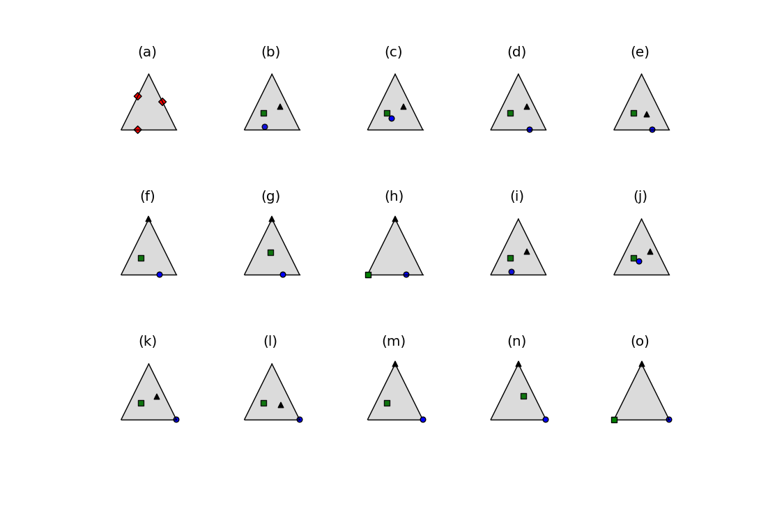
The Demix algorithm is recursive. Let $S_{1},\ldots,S_{K}$ denote $K$ contaminated distributions. In the base case, the algorithm takes as its input two contaminated distributions $S_{1}$ and $S_{2}$. It returns Residue($S_{1}\,|\,S_{2}$) and Residue($S_{2}\,|\,S_{1}$), which are a permutation of the two base distributions (see Figure 2). When $K>2$, Demix uses a subroutine FindFace (see Algorithm 5) to find $K-1$ distributions $R_{2},\ldots,R_{K}$ on the same $(K-1)$-face. FindFace iteratively generates candidates for distributions on the same $(K-1)$-face, which it tests using FaceTest (see Algorithm 6). FaceTest$(S_{1},\ldots,S_{K-1})$ determines whether a set of distributions $S_{1},\ldots,S_{K-1}$ are on the interior of the same face by using the two-sample $\kappa^{*}$ operator; equivalently, it tests whether there exists a pair of distributions $S_{i}$ and $S_{j}$ such that $S_{i}$ is irreducible with respect to $S_{j}$. Once Demix finds $K-1$ distributions $R_{2},\ldots,R_{K}$ on the same $(K-1)$-face, it recursively applies Demix to $R_{2},\ldots,R_{K}$ to obtain distributions $Q_{1},\ldots,Q_{K-1}$ that are a permutation of $K-1$ of the base distributions. Subsequently, the algorithm computes a maximizer $Q_{K}$ of $\kappa^{*}(\frac{1}{K}\sum_{i=1}^{K}S_{i}\,|\,Q_{1},\ldots,Q_{K-1})$. Since $Q_{1},\ldots,Q_{K-1}$ are a permutation of $K-1$ of the base distributions, the maximizer $Q_{K}$ is guaranteed to be unique and to be the remaining base distribution (see Figure 3 for an execution of the algorithm).

A number of remarks are in order regarding the Demix algorithm. First, although we compute the residue of $\frac{1}{n}S_{i}+\frac{n-1}{n}Q$ wrt $S_{1}$ for each $i\neq 1$, there is nothing special about the distribution $S_{1}$. We could replace $S_{1}$ with any $S_{j}$ where $j\in[K]$, provided that we adjust the rest of the algorithm accordingly. Second, we can replace the sequence $\{\frac{n-1}{n}\}_{n=1}^{\infty}$ with any sequence $\alpha_{n}\nearrow 1$. Finally, we could replace line 7 with the following sequence of steps: for $i=1,\ldots,K-1$, compute $Q_{K}\longleftarrow\text{Residue}(Q_{K}\,|\,Q_{i})$ (see Lemma 13). Then, the algorithm would only use the two-sample $\kappa^{*}$ operator. We use such an algorithm in the finite-sample setting.

We also remark that a simplified version of Demix solves the demixing mixed membership models problem if we assume (B1) from the multiclass label noise setting. In that case, finding $L-1$ distributions on the same face can be accomplished by simply computing $Q_{i}\longleftarrow\mathop{\textnormal{MultiResidue}}$($\tilde{P}_{i}\,|\,\{\tilde{P}_{j}\}_{j\neq i}$) for $i=2,\ldots,L$. Indeed, then, each $Q_{i}$ is equal to $P_{i}$ and $P_{1}$ can be obtained by computing $\mathop{\textnormal{MultiResidue}}(\tilde{P}_{1}\,|\,\{Q_{j}\}_{j=2,\ldots,L})$.

We establish the following theorem.

We briefly sketch three key aspects of the proof. First, in the FindFace subroutine, sampling $Q$ uniformly at random from $\mathop{\textnormal{conv}}(S_{2},\ldots,S_{K})$ ensures that w.p. 1 $\text{Residue}(Q\,|\,S_{1})$ is on the interior of a face of the simplex. Then, conditional on this event, we show that by a continuity property of $\text{Residue}(\cdot\,|\,S_{1})$ there is a large enough $n$ such that $R_{2},\ldots,R_{K}$ are on the same face of the simplex $\Delta_{K-1}$ (see panels (c) and (d) of Figure 3). Second, Proposition 8 in Appendix D establishes that the subroutine $\text{FaceTest}(R_{2},\ldots,R_{K})$ returns $1$ if and only if $R_{2},\ldots,R_{K}$ are on the same face of the simplex. Combining the above two observations implies that eventually FindFace($S_{1},\ldots,S_{K}$) terminates at which point $\{R_{k}\}_{k\in[K]\setminus\{1\}}\subset\{P_{k}\}_{k\in[K]\setminus\{l\}}$ for some $l\in[K]$. The final key observation is that $\{R_{k}\}_{k\in[K]\setminus\{1\}}$ and $\{P_{k}\}_{k\in[K]\setminus\{l\}}$ form an instance of the demixing problem that satisfies the sufficient conditions (A) and (B2) (see Figure 2). Therefore, this instance can be solved recursively.

As in the case of demixing mixed membership models, a simple resampling strategy works in certain nice settings of classification with partial labels. For example, consider an instance of classification with partial labels with the mixing matrix from equation (4). The resampling procedure that yields $\tilde{Q}_{1},\tilde{Q}_{2},\tilde{Q}_{3}$ (described in Section 4.4) also works here. Nevertheless, as in demixing mixed membership models, this approach does not meet our goal of an algorithm that solves a broad class of mixing matrices and partial labels.

Indeed, we observe that the partial labels do not provide enough information for choosing the resampling weights. Consider another instance of the problem with the same partial label matrix:

Applying the resampling approach to (5) can be shown to fail by observing that the inverse of the resampled mixing matrix does not satisfy condition 3 of Lemma 1. Thus, although the problem instances (4) and (5) have the same partial label matrix, the resampling procedure only works for one of these.

Next, we turn to presenting an algorithm that solves classification with partial labels for a wide class of mixing matrices and partial labels. We propose the PartialLabel algorithm (see Algorithm 7). PartialLabel proceeds by iteratively creating sets of candidate distributions $\bm{W}\coloneq(W_{1},\ldots,W_{L})^{T}$ via the subroutine CreateCandidates (see Algorithm 8). Given each $\bm{W}$, it runs an algorithm VertexTest (see Algorithm 9) that uses $\tilde{\bm{P}}$ and the partial label matrix $\bm{\Pi}^{+}$ to determine whether $\bm{W}$ is a permutation of the base distributions $\bm{P}$. If $\bm{W}$ is a permutation of $\bm{P}$, VertexTest constructs the corresponding permutation matrix for relating these distributions. If not, it reports failure and the PartialLabel algorithm increments $k$ and finds another set of candidate distributions.

The VertexTest algorithm proceeds as follows on a vector of candidate distributions $\bm{Q}\coloneq(Q_{1},\ldots,Q_{L})^{T}$. First, it determines whether there are two distinct distributions $Q_{i},Q_{j}$ such that $Q_{i}$ is not irreducible wrt $Q_{j}$, in which case $\bm{Q}$ cannot be a permutation of $\bm{P}$. If there is such a pair, it reports failure. Otherwise, it forms the matrix $Z_{i,j}\coloneq\bm{1}\{\kappa^{*}(\tilde{P}_{i}\,|\,Q_{j})>0\}$ and uses any algorithm that finds a permutation $\bm{C}$ (if it exists) of the columns of $\bm{Z}$ to match the columns of $\bm{\Pi}^{+}$. If such a permutation $\bm{C}$ exists, it returns $\bm{C}^{T}$ and, as we show in Lemma 7, $\bm{C}^{T}\bm{Q}=\bm{P}$; otherwise, VertexTest reports failure.

We remark that finding the permutation in line 6 of Algorithm 9 is not NP-hard. One algorithm (but most likely not the most efficient) proceeds as follows: define a total ordering on the columns of binary matrices. Sort the columns of $\bm{Z}$ and $\bm{\Pi}^{+}$ according to this total ordering. Check whether the resulting matrices are equal.

The following theorem gives our identification result for classification with partial labels.

There are two key ideas to the proof of Theorem 3. First, the randomization in line 2 of Algorithm 7 ensures through a linear independence argument that with probability $1$, the operation $\mathop{\textnormal{MultiResidue}}(\frac{1}{k}Q_{i}+(1-\frac{1}{k})\bar{Q}_{i}\,|\,\{Q_{j}\}_{j>i}\cup\{W_{j}\}_{j<i})$ in line 4 of Algorithm 8 is well-defined. Second, in the GenerateCandidates algorithm, let $Q_{j}=\bm{\tau}_{j}^{T}\bm{P}$ and $W_{j}=\bm{\gamma}_{j}^{T}P$. We make the simple observation that the affine hyperplane given by $\bm{\gamma}_{1},\ldots,\bm{\gamma}_{i-1},\bm{\tau}_{i+1},\ldots,\bm{\tau}_{L}$ bisects $\Delta_{L}$ such that $\bm{\tau}_{i}$ and a nonempty subset of $\{\bm{e}_{1},\ldots,\bm{e}_{L}\}\setminus\{\bm{\gamma}_{1},\ldots,\bm{\gamma}_{i-1}\}$ are in the same halfspace. Using this observation, we show that for large enough $k$, $W_{i}$ is one of the base distributions and is distinct from all $W_{j}$ with $j<i$.

References

- Arora et al. (2012) S. Arora, R. Ge, and A. Moitra. Learning topic models–going beyond svd. Foundations of Computer Science, 2012.
- Arora et al. (2013) S. Arora, R. Ge, Y. Halpern, D. Mimno, A. Moitra, D. Sontag, Y. Wu, and M. Zhu. A practical algorithm for topic modeling with provable guarantees. International Conference on Machine Learning, 2013.
- Axler (2015) S. Axler. Linear Algebra Done Right. Springer, 3rd edition, 2015.
- Berkman et al. (1989) L. Berkman, B. H. Singer, and K. Manton. Black/white differences in health status and mortality among the Elderly. Demography, 26:661–678, 1989.
- Blanchard and Scott (2014) G. Blanchard and C. Scott. Decontamination of mutually contaminated models. International Conference of Artificial Intelligence and Statistics, 2014.
- Blanchard et al. (2010) G. Blanchard, G. Lee, and C. Scott. Semi-supervised novelty detection. Journal of Machine Learning Research, 11:2973–3009, 2010.
- Blanchard et al. (2016) G. Blanchard, M. Flaska, G. Handy, S. Pozzi, and C. Scott. Classification with asymmetric label noise: Consistency and maximal denoising. Electronic Journal of Statistics, 10:2780–2824, 2016.
- Blei et al. (2003) D. Blei, A. Ng, and M. Jordan. Latent dirichlet allocation. Journal of Machine Learning research, 3:993–1022, 2003.
- Cid-Sueiro (2012) J. Cid-Sueiro. Proper losses for learning from partial labels. Advances in Neural Information Processing Systems, 2012.
- Cour et al. (2011) T. Cour, B. Sapp, and B. Taskar. Learning from partial labels. Journal of Machine Learning Research, 12:1501–1536, 2011.
- Das et al. (2015) R. Das, M. Zaheer, and C. Dyer. Gaussian lda for topic models with word embeddings. 2015.
- De Vito et al. (2010) E. De Vito, L. Rosasco, and A. Toigo. Spectral regularization for support estimation. Advances in neural information processing systems, 2010.
- Devroye et al. (1996) L. Devroye, L. Györfi, and G. Lugosi. A Probabilistic Theory of Pattern Recognition. Springer, 1996.
- Dheeru and K. Taniskidou (2017) D. Dheeru and E. K. Taniskidou. UCI machine learning repository, 2017. URL http://archive.ics.uci.edu/ml.
- Ding et al. (2013) W. Ding, M. Rohban, P. Ishwar, and V. Saligrama. Topic discovery through data dependent and random projections. International Conference on Machine Learning, 2013.
- Ding et al. (2014) W. Ding, M. Rohban, P. Ishwar, and V. Saligrama. Efficient distributed topic modeling with provable guarantees. International Conference on Artificial Intelligence and Statistics, 2014.
- Donoho and Stodden (2003) D. Donoho and V. Stodden. When does non-negative matrix factorization give a correct decomposition into parts? Advances in neural information processing systems, 2003.
- Fisher (1936) R.A. Fisher. The use of multiple measurements in taxonomic problems. Annual Eugenics, pages 179–188, 1936.
- Ghosh et al. (2017) A. Ghosh, H. Kumar, and P.S. Sastry. Robust loss functions under label noise for deep neural networks. AAAI, 2017.
- Huang et al. (2016) K. Huang, X. Fu, and N. D. Sidiropoulos. Anchor-free correlated topic modeling. Advances in Neural Information Processing Systems, 2016.
- Jain et al. (2016) S. Jain, M. White, M. W. Trosset, and P. Radivojac. Nonparametric semi-supervised learning of class proportions. arXiv preprint arXiv:1601.01944, 2016.
- Jin and Ghahramani (2002) R. Jin and Z. Ghahramani. Learning with multiple labels. Advances in Neural Information Processing Systems, 2002.
- LeCun et al. (1998) Y. LeCun, L. Bottou, Y. Bengio, and P. Haffner. Gradient-based learning applied to document recognition. IEEE, pages 2278–2324, 1998.
- Li et al. (2016a) C. Li, H. Wang, Z. Zhang, A. Sun, and Z. Ma. Topic modeling for short texts with auxiliary word embeddings. ACM SIGIR conference on Research and Development in Information Retrieval, 2016a.
- Li and Perona (2005) F. Li and P. Perona. A bayesian hierarchical model for learning natural scene categories. Computer Vision and Pattern Recognition, 2005.
- Li et al. (2016b) S. Li, T. Chua, and C. Miao. Generative topic embedding: a continuous representation of documents. ACL, 2016b.
- Liu and Dietterich (2012) L.-P. Liu and T. G. Dietterich. A conditional multinomial mixture model for superset label learning. Advances in Neural Information Processing Systems, 2012.
- Liu and Dietterich (2014) L.-P. Liu and T. G. Dietterich. Learnability of the superset label learning problem. International Conference on Machine Learning, 32, 2014.
- Luong et al. (2013) M. Luong, R. Socher, and C. Manning. Better word representations with recursive neural networks for morphology. Conference on Computational Natural Language Learning, 2013.
- Menon et al. (2015a) A. Menon, B. van Rooyen, C. Ong, and B. Williamson. Learning from corrupted binary labels via class-probability estimation. International Conference on Machine Learning, 2015a.
- Menon et al. (2015b) A. Menon, B. van Rooyen, C. S. Ong, and R. Williamson. Learning from corrupted binary labels via class-probability estimation. 2015b.
- Menon et al. (2016) A. Menon, B. van Rooyen, and N. Natarajan. Learning from binary labels with instance-dependent corruption. arXiv preprint, 2016.
- Metodiev and Thaler (2018a) E. Metodiev and J. Thaler. On the topic of jets. arXiv preprint arXiv:1802.00008, 2018a.
- Metodiev and Thaler (2018b) E. Metodiev and J. Thaler. Jet topics: Disentangling quarks and gluons at colliders. Physical Review Letters, 120(24):241602, 2018b.
- Natarajan et al. (2013) N. Natarajan, I. S. Dhillon, P. Ravikumar, and A. Tewari. Learning with noisy labels. Advances in Neural Information Processing Systems, 2013.
- Nyugen and Caruana (2008) N. Nyugen and R. Caruana. Classification with partial labels. International Conference on Knowledge Discovery and Data Mining, 2008.
- Patrini et al. (2017) G. Patrini, A. Rozza, A. Menon, R. Nock, and L. Qu. Making deep neural networks robust to label noise: a loss correction approach. CVPR, 2017.
- Pritchard et al. (2000) J. K. Pritchard, M. Stephens, N. A. Rosenberg, and P. Donnelly. Association mapping in structured populations. American Journal of Human Genetics, 67:170–181, 2000.
- Ramaswamy et al. (2016) H. Ramaswamy, C Scott, and A Tewari. Mixture proportion estimation via kernel embeddings of distributions. International Conference on Machine Learning, 2016.
- Recht et al. (2012) B. Recht, C. Re, J. Tropp, and V. Bittorf. Factoring non-negative matrices with linear programs. Advances in Neural Information Processing Systems, 2012.
- Rudi et al. (2014) A. Rudi, F. Odone, and E. De Vito. Geometrical and computational aspects of spectral support estimation for novelty detection. Pattern Recognition Letters, 2014.
- Sanderson and Scott (2014) T. Sanderson and C. Scott. Class proportion estimation with application to multiclass anomaly rejection. International Conference on Artificial Intelligence and Statistics, 2014.
- Scott (2015) C. Scott. A rate of convergence for mixture proportion estimation, with application to learning from noisy labels. International Conference on Artificial Intelligence and Statistics, 2015.
- Scott et al. (2013) C. Scott, G. Blanchard, and G. Handy. Classification with asymmetric label noise: Consistency and maximal denoising. Conference on Learning Theory, 2013.
- van Rooyen and Williamson (2015) B. van Rooyen and R. Williamson. Learning in the presence of corruption. arXiv preprint, 2015.
- van Rooyen et al. (2015) B. van Rooyen, A. Menon, and R. Williamson. Learning with symmetric label noise: The importance of being unhinged. Advances in Neural Information Processing Systems, 2015.
- Xun et al. (2017) G. Xun, Y. Li, W. X. Zhao, J. Gao, and A. Zhang. A correlated topic model using word embeddings. 2017.
- Zhao et al. (2018) H. Zhao, L. Du, W. Buntine, and M. Zhou. Inter and intra topic structure learning with word embeddings. 2018.